| Issue |
A&A
Volume 539, March 2012
|
|
|---|---|---|
| Article Number | A88 | |
| Number of page(s) | 16 | |
| Section | Astrophysical processes | |
| DOI | https://doi.org/10.1051/0004-6361/201117927 | |
| Published online | 28 February 2012 | |
Constraining Galactic cosmic-ray parameters with Z ≤ 2 nuclei
1 Laboratoire de Physique Subatomique et de Cosmologie, Université Joseph Fourier Grenoble 1, CNRS/IN2P3, Institut Polytechnique de Grenoble, 53 avenue des Martyrs, 38026 Grenoble, France
e-mail: coste@lpsc.in2p3.fr
2 The Oskar Klein Centre for Cosmoparticle Physics, Department of Physics, Stockholm University, AlbaNova, 10691 Stockholm, Sweden
Received: 22 August 2011
Accepted: 18 December 2011
Context. The secondary-to-primary B/C ratio is widely used for studying Galactic cosmic-ray propagation processes. The 2H/4He and 3He/4He ratios probe a different Z/A regime, which provides a test for the “universality” of propagation.
Aims. We revisit the constraints on diffusion-model parameters set by the quartet (1H, 2H, 3He, 4He), using the most recent data as well as updated formulae for the inelastic and production cross-sections.
Methods. Our analysis relies on the USINE propagation package and a Markov Chain Monte Carlo technique to estimate the probability density functions of the parameters. Simulated data were also used to validate analysis strategies.
Results. The fragmentation of CNO cosmic rays (resp. NeMgSiFe) on the interstellar medium during their propagation contributes to 20% (resp. 20%) of the 2H and 15% (resp. 10%) of the 3He flux at high energy. The C to Fe elements are also responsible for up to 10% of the 4He flux measured at 1 GeV/n. The analysis of 3He/4He (and to a lesser extent 2H/4He) data shows that the transport parameters are consistent with those from the B/C analysis: the diffusion model with δ ~ 0.7 (diffusion slope), Vc ~ 20 km s-1 (galactic wind), Va ~ 40 km s-1 (reacceleration) is favoured, but the combination δ ~ 0.2, Vc ~ 0, and Va ~ 80 km s-1 is a close second. The confidence intervals on the parameters show that the constraints set by the quartet data can compete with those derived from the B/C data. These constraints are tighter when adding the 3He (or 2H) flux measurements, and the tightest when the He flux is added as well. For the latter, the analysis of simulated and real data shows an increased sensitivity to biases. Using the secondary-to-primary ratio along with a loose prior on the source parameters is recommended to obtain the most robust constraints on the transport parameters.
Conclusions. Light nuclei should be systematically considered in the analysis of transport parameters. They provide independent constraints that can compete with those obtained from the B/C analysis.
Key words: methods: statistical / astroparticle physics / cosmic rays
© ESO, 2012
1. Introduction
Secondary species in Galactic cosmic rays (GCRs) are produced during the CR journey from the acceleration sites to the solar neighbourhood by means of nuclear interactions of heavier primary species with the interstellar medium (ISM). Hence, they are tracers of the CR transport in the Galaxy (e.g., Strong et al. 2007). Studying secondary-to-primary ratios is useful because it factors out the “unknown” source spectrum of the progenitor, leaving 2H/4He, 3He/4He, B/C, sub-Fe/Fe – and recently  (Putze et al. 2009; di Bernardo et al. 2010) – suitable quantities for constraining the transport parameters for species Z ≤ 30.
Most secondary-to-primary ratios have A/Z ~ 2, and in that respect, 3He/4He is unique because it probes a different regime and allows one to address the question of the “universality” of propagation histories. For instance, in an analysis in the leaky-box model (LBM) framework, Webber (1997) found that 3He/4He data imply a similar propagation history for the light and heavier species (which was disputed in earlier papers). Webber also argued that the situation with regard to the 2H/4He ratio is less clear, because the uncertainties on the measurements are large (mainly caused by instrumental and atmospheric corrections). H and He spectra are the most abundant species in the cosmic radiation, and thus 2H and 3He are the most abundant secondary species in GCRs. However, achieving a good mass resolution – especially at high energy – is experimentally challenging. This explains why the elemental B/C ratio received more focus both experimentally and theoretically (thanks to its higher precision data w.r.t. to the quartet data).
From the modelling side, after the first thorough and pioneering studies performed in the 60’s–70’s (Badhwar & Daniel 1963; Ramaty & Lingenfelter 1969; Meyer 1972; Mitler 1972; Ramadurai & Biswas 1974; Mewaldt et al. 1976), the interest for the quartet nuclei somewhat stalled. Several updated analyses of the propagation parameters from the quartet were published whenever new data became available (see Table A.1 for references). However, very few dedicated studies were carried out in the 1980s (Beatty 1986; Webber et al. 1987) or 1990s (Webber 1990a; Seo & Ptuskin 1994; Webber 1997), and none in the first decade of this century. This is certainly related to the very slow pace at which new data became available in this period. Curiously, the most recent published data have not really been properly interpreted, i.e. for 2H/4He data, IMAX92 (de Nolfo et al. 2000) and AMS-01 (Aguilar et al. 2011); and for 3He/4He data, IMAX92 (Menn et al. 2000), SMILI-II (Ahlen et al. 2000), AMS-01 (Xiong et al. 2003), BESS98 (Myers et al. 2003), CAPRICE98 (Mocchiutti et al. 2003). Furthermore, almost all analyses have been performed in the successful but simplistic LBM except for a few studies1. At the same time, the analysis of the B/C ratio has been scrutinised in greater detail. For instance, to replace the old usage of matching the data by means of an inefficient manual scan of the parameter space (e.g., Jones et al. 2001), more systematic scans were carried out (on the B/C and sub-Fe/Fe ratio) to get best-fit values as well as uncertainties on the parameters (Maurin et al. 2001; Lionetto et al. 2005; Evoli et al. 2008; di Bernardo et al. 2010). A recent improvement is the use of Markov Chain Monte Carlo (MCMC) techniques to directly access the probability-density function (PDF) of the GCR transport and source parameters (Putze et al. 2009, 2010, 2011; Trotta et al. 2011).
In this paper, we revisit the constraints set by the quartet nuclei and their consistency with the results of heavier nuclei. In the context of the forthcoming PAMELA and AMS-02 data on these ratios, we also discuss the strategy to adopt and intrinsic limitations of the transport parameters reconstruction. For that purpose, we take advantage of the data taken in the last decade as well as simulated data of any precision, and analyse them with an MCMC technique implemented in the USINE propagation code. This extends and complements analyses of the B/C and primary nuclei (Putze et al. 2010, 2011) in a 1D diffusion model.
The paper is organised as follows. In Sect. 2, we briefly recall the main ingredients of the 1D diffusion model and the MCMC analysis. We also list the parameters that are constrained. The simulated data and their analysis are described in Sect. 3. The analysis of the real data is given in Sect. 4. We conclude in Sect. 5. Appendix A gathers the data sets and the updated cross-sections used in the quartet analysis.
2. MCMC technique, propagation and parameters
The MCMC technique and its use in the USINE propagation code is detailed in Putze et al. (2009) and summarised in Putze et al. (2010). The full details regarding the 1D transport model can be found in Putze et al. (2010). Below, we only provide a brief description.
2.1. An MCMC technique for the PDF of the parameters
The MCMC method, based on Bayesian statistics, is used to estimate the full distribution (conditional PDF) given some experimental data and some prior density for these parameters. Our chains are based on the Metropolis-Hastings algorithm, which ensures that the distribution of the chain asymptotically tends to the target PDF.
The chain analysis refers to the selection of a subset of points from the chains (to obtain a reliable estimate of the PDF). The steps at the beginning of the chain are discarded (burn-in length) if they are too far of the region of interest. Sets of independent samples are obtained by thinning the chain (over the correlation length). The final results of the MCMC analysis are the joint and marginalised PDFs. They are obtained by counting the number of samples within the related region of the parameter space.
2.2. 1D Propagation model and parameters
The Galaxy is modelled to be an infinite thin disc of half-thickness h, which contains the gas and the sources of CRs. The diffusive halo region (where the gas density is assumed to be equal to 0) extends to + L and − L above and below the disc. A constant wind V(r) = sign(z)·Vc × ez, perpendicular to the Galactic plane, is assumed. In this framework, CRs diffuse in the disc and in the halo independently of their position. Such semi-analytical models are faster than full numerical codes (GALPROP2 and DRAGON3), which is an advantage for sampling techniques like MCMC approaches.
2.2.1. Transport equation
The differential density Nj of the nucleus j is a function of the total energy E and the position r in the Galaxy. Assuming a steady state, the transport equation can be written in a compact form as 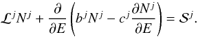 (1)The operator ℒ (we omit the superscript j) describes the diffusion K(r,E) and the convection V(r) in the Galaxy, but also the decay rate Γrad(E) = 1/(γτ0) if the nucleus is radioactive, and the destruction rate Γinel(r,E) = ∑ ISMnISM(r)vσinel(E) for collisions with the ISM, in the form
  (2)The coefficients b and c in Eq. (1) are first- and second-order gains/losses in energy, with
 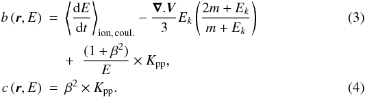 In Eq. (3), the ionisation and Coulomb energy losses are taken from Mannheim & Schlickeiser (1994) and Strong & Moskalenko (1998). The divergence of the Galactic wind V gives rise to an energy-loss term related to the adiabatic expansion of cosmic rays. The last term is a first-order contribution in energy from reacceleration. Equation (4) corresponds to a diffusion in momentum space, leading to an energy gain. The associated diffusion coefficient Kpp (in momentum space) is taken from the model of minimal reacceleration by the interstellar turbulence (Osborne & Ptuskin 1988; Seo & Ptuskin 1994). It is related to the spatial diffusion coefficient K by
 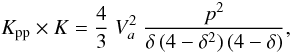 (5)where Va is the Alfvénic speed in the medium.
We refer the reader to Appendix A of Putze et al. (2010) for the solution to Eq. (1) in the 1D geometry.
2.2.2. Free parameters of the analysis
The exact energy dependence of the source and transport parameters is unknown, but they are expected to be power laws of ℛ = pc/Ze (rigidity of the particle).
The low-energy diffusion coefficient requires a β = v/c factor that takes into account the inevitable effect of particle velocity on the diffusion rate. However, the recent analysis of the turbulence dissipation effects on the transport coefficient has shown that this coefficient could increase at low-energy (Ptuskin et al. 2006; Shalchi & Büsching 2010). Following Maurin et al. (2010), it is parametrised to be 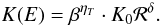 (6)The default value used for this analysis is ηT = 1. The two other transport parameters are Vc, the constant convective wind perpendicular to the disc, and Va, the Alfvénic speed regulating the reacceleration strength (see Eq. (5)). The two models considered in this paper are given in Table 1.
Models tested in the paper.
The low-energy primary source spectrum from acceleration models (e.g., Drury 1983; Jones 1994) is also unknown. We parametrise it to be  (7)where q is the normalisation. The reference low-energy shape corresponds to ηS = −1 (to have dQ/dp ∝ p − α, i.e. a pure power-law).
The halo size of the Galaxy L cannot be solely determined from secondary-to-primary stable ratios and requires a radioactive species to lift the degeneracy between K0 and L. However, the range of allowed values is still very loosely constrained (e.g., Putze et al. 2010). Because the transport and source parameters can always be rescaled if a different choice of L were assumed (see the scaling relations given in Maurin et al. 2010, where δ is shown not to depend on L), we fixed it to L = 4 kpc. This will also facilitate the comparison of the results obtained in this paper with those of our previous studies (Putze et al. 2010, 2011).
3. MCMC analysis on artificial data sets
MCMC techniques make the scan of high-dimensional parameter spaces possible, such that a simultaneously estimation of transport and source parameters is possible (Putze et al. 2009). However, transport parameters are shown to be strongly degenerated for the B/C ratio data in the range 0.1−100 GeV/nuc (Maurin et al. 2010), and source and transport parameters are correlated (Putze et al. 2009, 2010). For GCR data in general, the fact that primary fluxes and secondary fluxes are not measured to the same accuracy4 can bias or prevent an accurate determination of these parameters: a simultaneous fit has been observed to be driven by the more accurately measured primary flux (Putze et al. 2011). This, although statistically correct, might not maximise the information obtained on the transport parameters. Therefore, several strategies can be considered when dealing with GCR data:
-
a combined analysis of secondary-to-primary ratio and primaryflux to constrain the source and transport parameterssimultaneously;
-
a secondary-to-primary ratio analysis only, either fixing the source parameters (i.e., using a strong prior), or using a loose prior;
-
a primary flux analysis only, either fixing the transport parameters (i.e., using a strong prior), or using a loose prior.
In the literature, the strong prior approach has almost always been used to determine the transport or the source parameters. The question we wish to address is how sensitive the parameters of interest are to various strategies. This is the motivation for introducing artificial data, i.e. an ideal case study, as opposed to the case of real data where several other complications can arise (systematics in the data and/or the use of the incorrect propagation model or solar modulation model/level).
3.1. Sets of artificial data
MCMC analysis on simulated data.
To be as realistic as possible, we chose models that roughly reproduce the actual data points (see Fig. 4), but also match the typical energy coverage, number of data points, central value and spread (error bars) of the measurements5. To speed-up the calculation and for this section only, we assume that all 3He comes from 4He (see Sect. 4.1 for all relevant progenitors). No systematic errors were added, although they may set a fundamental limitation in recovering the cosmic-ray parameters. In practice, the statistical errors for the artificial data sets correspond to the sigma of the standard Gaussian deviations used to randomise the data points around their model value: 3He/4He was generated with statistical errors of 10% while He fluxes were generated with 1% and 10% errors, to simulate the situation where primary fluxes are “more accurately” or “equally” measured (in terms of statistics) than the secondary-to-primary ratio.
The parameters of the two models used to simulate the data are listed in the two italic lines in Table 2, denoted Model II and Model III. They correspond to extreme values of the diffusion slope δ, but which still roughly fall in the range of values found for instance from the B/C analysis (Putze et al. 2010): for Model II with reacceleration only (Vc = 0), δ is generally found to fall between 0.1 and 0.3, whereas for Model III with convection and reacceleration, δ is generally found to fall into the 0.6 − 0.8 range (Jones et al. 2001; Maurin et al. 2010).
3.2. Strategies to analyse the data
To test the impact on the reconstruction of the transport (ηT, K0, δ, Va, and Vc) and/or source (α and ηS) parameters, we tested the following combinations (data set|model parameters) for the analysis.
3He/4He + He data
-
Option 1 (σHe = 10%):
transport + source;
-
Option 2 (σHe = 1%):
transport + source;
-
Option 2’ (σHe = 1%):
transport (source = “true” value);
3He/4He ratio only
-
Option 3:
transport + source;
-
Option 3’:
transport (source = “true” value);
-
Option 4:
transport (source = weak prior).
We find that the He data alone cannot constrain the transport parameters (not shown here), in agreement with the Putze et al. (2011) results (strong degeneracy between α and δ, but also with K0, Va, and ηT).
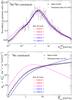 |
Fig. 1 Analysis of simulated interstellar (IS) data sets for the 3He/4He ratio (top panel) and the 4He flux times |

3.3. Analysis of the artificial data
In a first step, we used the MCMC technique to estimate the best-fit parameters. The 3He/4He ratio and 4He flux are shown for model II (crosses) and the corresponding simulated data (pluses) in Fig. 1. When both the 3He/4He and 4He data are included in the fit (options 1 and 2, red dotted and red solid lines), the initial flux (crosses) is perfectly recovered for 4He, and very well recovered for 3He/4He. When the fit is only based on 3He/4He (options 3 and 5, magenta dashed and blue solid lines), the initial flux is obviously not recovered (unless the source parameters are set to the true value as in option 3’), but the 3He/4He ratio is consistent with the data. Unsurprisingly, the associated  /d.o.f. values (last column of Table 2) are close to 1.
The MCMC analysis allows us to go further because it provides the PDF of the parameters from which the most probable value and confidence intervals (CIs) are obtained. The results are gathered in Table 2 and Fig. 2. The various panels of the latter represent the PDFs for transport and source parameters for each “option” for Model II. (For clarity the correlation plots are not shown.)
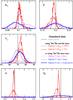 |
Fig. 2 Marginalised posterior PDF for the transport and source parameters on the artificial data for Model II (the values for the input model are shown as thick vertical grey lines in each panel). The colour code and style correspond to the five “options” described in Sect. 3.2 (same as in Fig. 1). |
From these plots, some arguments are in favour of a simultaneous use of the secondary-to-primary ratio and the primary flux (here, 3He/4He and He), but not all.
3.3.1. Advantages from a simultaneous analysis (ratio + flux)
A simultaneous analysis (3He/4He + He) gives more stringent constraints on the transport parameters than an analysis of the secondary-to-primary ratio (compare the PDFs for the red curves and blue curves in Fig. 2 respectively, for K0, δ, and Vc). This partly comes from the observed correlations between transport and source parameters6 (e.g., Putze et al. 2009). Option 2’ and option 3’ with fixed source parameters show that the better CIs on the transport parameters come from the information contained in primary fluxes7. The same conclusions hold true for Model III (Vc ≠ 0), although with larger relative uncertainties bevause of the two extra transport parameters of the model (ηT and Vc).
3.3.2. What if the wrong model is used?
As an illustration, we analysed data simulated from model III (Vc ≠ 0) with model II (Vc = 0) and vice versa (lower half of Table 2). If we force Vc = 0 (while  km s-1), the diffusion slope decreases to a low value δ ~ 0.2 (δtrue = 0.7), while the Alfvénic speed increases to a high value Va ~ 100 km s-1 (
 km s-1). The higher /d.o.f. value with respect to the one obtained fitting the correct model easily disfavours this model. The second test (simulated with II, analysed with III) indicates whether allowing for more freedom in the analysis (two additional free parameters ηT and Vc) affects the recovery of the parameters. The values of δtrue = 0.2 and
  km s-1 are recovered, while the others are systematically offset but less than 3σ away from their true value. In this simple example, adding extra parameters is not a problem because the /d.o.f. still favours the minimal model. However, with real data (see Sect. 4.3 and the B/C analysis of Putze et al. 2010; Maurin et al. 2010) it is so far impossible in this situation to conclude whether the correct model is used because of the possible problem of multimodality and biases from systematics (see below).
3.3.3. Drawbacks of a simultaneous analysis
For Model II, but even more for Model III (which has more free transport parameters), a possible worry is the presence of multimodal PDF distributions, which more often happens for the simultaneous analysis. An example of multimodality is the analysis with Model II (i.e. Va = 0) of data simulated with Model III, which corresponds to a local minimum of the true Model III parameters. This is of no consequence for the ideal case, but real data may suffer from systematics errors and/or the inappropriate solar modulation model may be chosen. In that case, the true minimum can be displaced, or turned into a local minimum (and vice versa). Measurements over the past decades showed that primary fluxes are more prone to systematics than secondary-to-primary ratios. Primary fluxes are also more sensitive to solar modulation than ratios. For these reasons, the use of secondary-to-primary data only (option 4) for the analysis, although they perform less well in obtaining stringent limits on the transport parameters, is expected to be more reliable and robust.
Estimated fractional contribution of projectile A > 4 to the 2H and 3He fluxes.
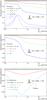 |
Fig. 3 Fractional contributions to the propagated 2H fluxes (top panel), 3He fluxes (middle panel) and 4He fluxes (bottom panel) as a function of Ek/n from A > 4 CR parents. For 4He, the primary contribution is also considered. |
3.4. Recommended strategy for analysing real data
The most robust approach to determine the transport parameters (and their CIs) is to analyse the secondary-to-primary ratio using a loose but physically-motivated prior on the source parameters (option 4). This has the advantage of taking into account the correlations between the source and transport parameters. The simultaneous analysis is mandatory to obtain the source parameters (option 1 or 2). It also yields more information on the transport parameters, but the primary fluxes can bias their determination if it suffers from systematics. We recommend such an analysis to be performed in addition to the direct secondary-to-primary ratio analysis, in order to obtain the following diagnosis: if the range of values for the transport parameters from both analyses are
-
inconsistent, it indicates that the values and CIs obtained for thesource parameters are biased or unreliable;
-
consistent, the selected propagation model may be the correct one, and the source parameters are then the most probable ones for this model. However, the CIs on the transport parameters are very likely to be underestimated if the error bars on the ratio are much larger than those on the primary fluxes.
Obviously, our analysis does not cover the range of all systematics when dealing with real data. A more systematic analysis – e.g. covering a wider family of propagation models, several solar modulation models, several sources of systematics in the data – goes far beyond the scope of this paper. Note that some of these effects are likely to be energy dependent, which complicates the analysis even more. With the successful installation of the AMS-02 detector on the ISS and its expected high-precision data, these problems are bound to gain importance.
4. Constraints from the quartet data
We now apply the MCMC technique to the analysis of real data. We emphasise that for the artificial data, we assumed the 3He to come solely from the 4He fragmentation to speed up the calculation. Based on our new compilation for the cross-section formulae (see Appendix B), we included the contributions from A > 4 CR parents, checking which parents are relevant (Sect. 4.1). After determining the heaviest parent to consider in the calculation, we then move on to the result of the MCMC analysis (Sect. 4.2), and those from our best analysis (Sect. 4.3).
4.1. Fractional contributions
At first order, the contribution to the 2H and 3He secondary production from Z > 4 nuclei is proportional to the source term  (see Eq. (1)). For a secondary contribution, the source term is proportional to the primary flux of the parents (which have been measured by many experiments), and to the production cross-section. Normalised to the production from 4He, we have
 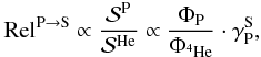 (8)where P is the CR projectile, S is the secondary fragment considered, and
  (see Eq. (B.3)) is the production cross-section relative to the production from 4He. The fractional contribution fP → S for each parent is defined to be
 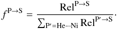 (9)As seen from Table 3, the most important contributions from primary species heavier than He (Z > 2) are C and O, followed by Mg and Si and finally Fe. The total contribution of these species amounts to ~35% for 2H and ~11% for 3He, but mixed species (such as N) or less abundant species also contribute to ~5%.
A proper calculation of these fractional contributions involves the full solution of the propagation equation, taking into account energy gains and losses, total inelastic reactions, and convection. Based on the propagation parameters found to fit the current data best (see next section), we show in Fig. 3 the fractional contribution of A > 4 nuclei as a function of energy for the full calculation. It confirms the previous figures, but with a residual energy dependence (itself depending on the species) hitting a plateau above ~100 GeV/n. The difference can be mostly attributed to a preferential destruction of heavier nuclei at low energy8. Note that for 2H production, the coalescence of two protons (long-dashed pink curve) contributes up to 40% of the total at ~1 GeV/n energy (peak of the cross-section, see Fig. B.3). Depending on the precision reached for the data, it is important to include the CNO contribution (e.g. Ramaty & Lingenfelter 1969; Jung et al. 1973b; Beatty 1986), but also all contributions up to Ni.
Finally, the fragmentation of CNO can also affect the 1H and 4He primary fluxes. The peak of contribution occurs at GeV/n as secondary fluxes drop faster than primary fluxes with energy. Figure 3 shows this contribution to be ≲ 10% for 4He. With the high precision measurement from PAMELA and the even better measurements awaited from AMS-02, this will need to be further looked into in the future.
MCMC analysis of Model III (with L = 4 kpc) from various quartet data subsets.
4.2. MCMC analysis: test of several data combinations
Given the accuracy of current data (see Fig. 4), we must take into account the contribution from all parent nuclei at least up to 30Si. In the rest of the analysis, we use PAMELA data for He (Adriani et al. 2011), as they overcome all others in the ~GeV−TeV range in terms of precision. Before giving our final results, and to complement Sect. 3.2, we discuss the appropriate choice of data to consider here, in order to get the best balance between robustness and reliability for the 2H and 3He-related analyses.
4.2.1. Simulated vs. real data
We start by comparing the results obtained with the simulated and the actual data set. To avoid lengthy comparisons of numbers, we limit ourselves to Model III (where we also fix ηT to its default value, i.e. 1). The obvious difference with the simulated data is that we no longer have access to the true source parameters (automatically excluding options 2′ and 4 discussed in Sect. 3.2). For the simultaneous analysis using He PAMELA data – the precision of which is ~1% –, we recover similar values and CIs for the parameters (compare option 2 in Table 2 and the first three lines of Table 4). The second row of Table 4 is based on a subset of He data: high-energy data points are discarded because they show departure from a single power-law (Ahn et al. 2010; Adriani et al. 2011), whereas low-energy data points are discarded because of their sensitivity to solar modulation, which is presumably too crudely described by the Force-Field approximation used here. The /d.o.f. value (first row) shows that the model has difficulties to perfectly match the high precision PAMELA He data over the whole energy range. The analysis of 3He/4He ratio using a prior on the source parameters (option 4 in Table 2 and third line of Table 4) gives higher CIs for the transport parameters. The consistency between the results of the latter analysis (third line) and that based on the partial He data (second line), and their discrepancy with the results of the analysis based on the full He data set (first line) confirms our suspicion that high-precision measurements for primary fluxes can bias the transport parameter determination.
4.2.2. Adding the secondary 3He flux in the analysis
Replacing He by 3He in the simultaneous analysis (4th and 5th line) affects the determination of the transport parameters even more. This is not surprising since 3He data are not all consistent with one another (see Fig. 4). The bias is stronger when taking into account the recently published AMS-01 data (Aguilar et al. 2011). If both 3He and He are taken into account9, the much better accuracy of the He PAMELA data with respect to the 3He data amounts to a smaller weight of the latter in the analysis.
4.2.3. 2H/4He vs. 3He/4He
We partially repeated the analysis for 2H in the last three rows of Table 2. The data are so inconsistent with each other for 2H/4He (see Fig. 4) that we were forced to use at least the 2H flux (whose data points are also markedly inconsistent with each other). Even so, the results are not reliable. PAMELA and AMS-02 have the capability to improve greatly the situation, but in the meantime, we are forced to include He as well in the analysis (next-to-last row in the table). The transport parameter values from the 2H/4He+2H+He analysis are mostly consistent with those from the 3He/4He+3He+He analysis, but are likely to suffer from similar biases (see the previous paragraph). Reducing the energy range of He data is not even possible for the 2H analysis (last line in the table), because the obtained results are not reliable.
4.3. MCMC analysis: “best” results
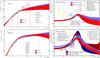 |
Fig. 4 Left panels: demodulated interstellar 2H (top) and 3He (bottom) envelopes at 95% CIs times |

Taking into account the specifics of the actual data (previous section), our “best” analysis is based on the most relevant combinations of data for 2H and 3He:
-
the 3He/4He analysis (with a prior for the source parameters)gives robust and conservative results for the transportparameters. The result from the3He/4He+3He+He analysis is more sensitive to biases, but using an energy sub-range for He data is expected to limit them;
-
owing to the paucity of 2H data, the 2H/4He+2H+He (full energy-range for He) analysis is the only reliable option, although it probably suffers from biases.
The corresponding most probable values and CIs are gathered in Table 5, and the corresponding envelopes for 2H/4He, 2H, 3He/4He, and 3He/4He are given in Fig. 4. We also re-analysed the B/C ratio according to our “best-analysis” scheme (B/C alone with a prior for the source parameters or B/C + C). The results are reported in Table 5, where the results obtained in Putze et al. (2010) for fixed source parameters are also reproduced: we note that the new strategy yields results that agree better with those of the quartet analysis (e.g., the transport parameters δ and K0 are shifted by more than 30% for Model II), which again demonstrates its usefulness.
4.3.1. Universality of the transport parameters
If we focus on the transport parameters, we note that combinations involving the 2H/4He, 3He/4He, or B/C ratio yield broadly consistent transport parameter values, be it for Model II or Model III10. Regardless of the actual propagation model, we conclude that these results hint at the universality of CR transport for all species. Another important result is that the constraints set by the quartet data on the transport parameters can compete with those set by the B/C ratio, so that the quartet data should be a prime target for AMS-02.
4.3.2. Model II (δ ~ 0.3) or Model III (δ ~ 0.7)?
According to Sect. 3.2, comparing the results of the secondary-to-primary ratio analysis with those of the combined analysis (ratio + primary flux) gives an indication of their robustness. Table 5 shows that the results for the diffusion slope δ is very robust, regardless of the model considered. A more detailed comparison shows that for 3He-related constraints, the transport parameter values for Model II are inconsistent with each other at the 3σ level, whereas the 68% CIs overlap with one another (but for Vc) for Model III, hence slightly favouring the latter (δ ~ 0.7). The comparison of the /d.o.f. values also tends to favour model III. Hence, although the value δ ~ 0.7 seems favoured, we cannot exclude a pure reacceleration model (Vc = 0) with δ ~ 0.3 yet. Moreover, as shown in Maurin et al. (2010), many ingredients of the propagation models can lead to a systematic scatter of the transport parameters larger than the width of their CIs. Data at higher energy for any secondary-to-primary ratio are mandatory to conclude on this question.
4.3.3. Source spectrum
The present analysis is more general than that used in Putze et al. (2011), where the transport parameters were fixed. Although it is not the main focus of this paper, we remark that the values of the source slope α from the B/C + C analysis are consistent with those found in Putze et al. (2011), strengthening the case of a universal source slope α at the ~ 5% level. For the quartet values, αHe is broadly consistent with Putze et al.’s analysis (based on AMS-01, BESS98 and BESS-TeV data for He). However, the results for the source parameters depend on the choice of data sets and energy range considered. This indicates that for ≲ 1% accuracy data, either the model for the source is inappropriate, or the solar modulation model is faulty, or some systematics exist in the measurements. The AMS-02 data will help to clarify this question.
5. Conclusion
We have revisited the constraints set on the transport (and also the source) parameters by the quartet data, i.e. 1H, 2H, 3He, and 4He fluxes, but also the secondary-to-primary ratios 2H/4He and 3He/4He. This extends and complements a series of studies (Putze et al. 2009, 2010, 2011) carried out with the USINE propagation code and an MCMC algorithm. The three main ingredients on which the analysis rests are
-
A minute compilation of the existing quartet data and survey of theliterature, showing that the most recent/precise data (AMS-01,BESS93 → 98, CAPRICE98, IMAX92, and SMILI-II) have not been considered before this analysis.
-
We performed a systematic survey of the literature for the cross-sections involved in the production/survival of the quartet nuclei. This has lead us to propose new empirical production cross-sections of 2H, 3H, and 3He, valid above ~30 MeV/n for any projectile on p and He (we also updated inelastic cross-sections).
-
We extensively used artificial data sets to assess the reliability of the derived CIs of the GCR transport and source parameters for various combinations of data/parameter analyses.
In broad agreement with previous studies, (e.g. Ramaty & Lingenfelter 1969; Beatty 1986), we find that the fragmentation of CNO contributes significantly to the 2H flux (~30%) above a few GeV/n energies (4He fragmentation is the dominant channel for the 2H and 3He fluxes). Nevertheless, we provided a much more detailed picture, showing in particular that heavy nuclei (8 < Z ≤ 30) contribute up to 10% for 3He (20% for 2H) at high energy. We also provided an estimate of the secondary fraction to the 4He flux. By definition, the secondary contribution has a steeper spectrum than the primary one and therefore quickly becomes negligible at high energy. This secondary contribution peaks at a few GeV/n, and amounts to ~10% of the total flux (~7% up to O fragmentation, ~2% from elements heavier than O), which is already a sizeable amount given the ~1% precision reached by the PAMELA data (Adriani et al. 2011). For 1H, the knowledge of the multiplicity of neutron and proton produced by the interaction of all elements on the ISM is required to calculate its secondary content precisely.
Simulated data have allowed us to check several critical behaviours. Firstly, the He flux is obviously useful (and required) to constrain the source parameters, but it has also been found to bring significant information on the transport parameters: fitting a secondary-to-primary ratio plus a primary flux brings more constraints than just fitting the ratio (even when source parameters are fixed). Secondly, we have checked that a model with more free parameters (than those used to simulate the data) is able to recover the correct values. However, our analysis has also strongly hinted that adding the primary flux He biases the determination of the transport parameters if systematics (which are usually more important in primary fluxes than in ratios) are present, and/or if the wrong model is used. For this reason, when dealing with measurements, we recommend to always compare the result from the secondary-to-primary ratio + primary flux analysis to that of the secondary-to-primary ratio using a loose but physically motivated prior on the source parameters.
The analysis of real data has shown that quartet data slightly favour a model with large δ ~ 0.7 (with Vc ~ 20 km s-1 and Va ~ 40 km s-1), but that a model with small δ ~ 0.2 (with Vc ~ 0 and Va ~ 80 km s-1) cannot be completely ruled out. Better quality data, and especially data at higher energy are required to proceed. The conclusions are similar and the range of transport parameters found are consistent with those obtained from the B/C analysis (Jones et al. 2001; Putze et al. 2010; Maurin et al. 2010)11. This strongly hints at the the universality of the GCR transport for all nuclei. Furthermore, we have shown that the analysis of the light isotopes (and the already very good precision on He) is as constraining as the B/C analysis (similar range of CIs).
The several difficulties that we pointed out in this analysis could be solved by using better data. However, it is more likely that the interpretation of future high-precision data will require the development of refined models for the source spectra and/or transport and/or solar modulation. For instance, the force-field approximation for solar modulation is already too crude to precisely match the PAMELA He data. The forthcoming AMS-02 data at an even better accuracy will definitively pose interesting new challenges.
Seo & Ptuskin (1994) used a 1D diffusion model with reacceleration, whereas Webber & Rockstroh (1997) relied on a Monte Carlo calculation; both studies conclude in a similar way (consistency with the grammage required for heavier species to produce the light secondaries). A preliminary effort based on the GALPROP propagation code was also carried out in Moskalenko et al. (2003).
The uncertainty on the H and He fluxes is a few percent (for the recent PAMELA data, Adriani et al. 2011) and 20–50% for the 3He/4He ratio.
Note that the lack of constraints on the source parameters for option 4 confirms that the secondary-to-primary ratio is only marginally sensitive to the source parameters (e.g., Putze et al. 2011).
Indeed, the primary-to-primary ratios are not constant. The heavier the nucleus, the larger its destruction cross-section, the more the propagated flux is affected/decreased at low energy, the longer it takes to reach a plateau of maximum contribution at high energy. The observed trend is consistent with the primary-to-primary ratios shown in Fig. 14 of Putze et al. (2011).
The simultaneous analysis of 3He/4He + 3He + He was not tested in the simulated data since it would have amounted to a double-counting of the 3He data (appearing in the three quantities). However, real data involve different experiments for the various quantities (PAMELA for He and other experiments for 3He), and independent measurements were used.
The most significant difference is for the 2H/4He+2H+He analysis, which is inconsistent in both models and clearly unreliable for Model II (δ ~ 0). For model III, B/C and 3He/4He-related constraints are roughly in the same region but are located at several σ from each other (they are consistent with each other for Model II).
Acknowledgments
D.M. would like to thank A. V. Blinov for kindly providing copies of several of his articles. A.P. is grateful for financial support from the Swedish Research Council (VR) through the Oskar Klein Centre.
References
- Abdullin, S. K., Blinov, A. V., Vanyushin, I. A., et al. 1993, Phys. Atom. Nucl., 56, 536 [NASA ADS] [Google Scholar]
- Abdullin, S. K., Blinov, A. V., Chadeeva, M. V., et al. 1994, Nucl. Phys. A, 569, 753 [NASA ADS] [CrossRef] [Google Scholar]
- Ableev, V. G., Bodyagin, V. A., Zaporozhets, S. A., et al. 1977, JINR-P1-10565 [Google Scholar]
- Adriani, O., Barbarino, G. C., Bazilevskaya, G. A., et al. 2011, Science, 332, 69 [NASA ADS] [CrossRef] [PubMed] [Google Scholar]
- Aguilar, M., Alcaraz, J., Allaby, J., et al. 2011, ApJ, 736, 105 [NASA ADS] [CrossRef] [Google Scholar]
- Ahlen, S. P., Greene, N. R., Loomba, D., et al. 2000, ApJ, 534, 757 [NASA ADS] [CrossRef] [Google Scholar]
- Ahn, H. S., Allison, P. S., Bagliesi, M. G., et al. 2008, Astropart. Phys., 30, 133 [Google Scholar]
- Ahn, H. S., Allison, P., Bagliesi, M. G., et al. 2010, ApJ, 714, L89 [Google Scholar]
- Aladashvill, B., Bano, M., Braun, H., et al. 1981, Acta Physica Slovaca, 31, 29 [Google Scholar]
- Ammon, K., Leya, I., Lavielle, B., et al. 2008, Nucl. Inst. Meth. Phys. Res. B, 266, 2 [Google Scholar]
- AMS Collaboration 2002, Phys. Rep., 366, 331 [NASA ADS] [CrossRef] [Google Scholar]
- Apparao, K. M. V. 1973, in International Cosmic Ray Conference, 1, 126 [Google Scholar]
- Badhwar, G. D., & Daniel, R. R. 1963, Progr. Theoret. Phys., 30, 615 [NASA ADS] [CrossRef] [Google Scholar]
- Beatty, J. J. 1986, ApJ, 311, 425 [NASA ADS] [CrossRef] [Google Scholar]
- Beatty, J. J., Garcia-Munoz, M., & Simpson, J. A. 1985, ApJ, 294, 455 [NASA ADS] [CrossRef] [Google Scholar]
- Beatty, J. J., Ficenec, D. J., Tobias, S., et al. 1993, ApJ, 413, 268 [Google Scholar]
- Bieri, R. H., & Rutsch, W. 1962, Helv. Phys. Acta, 35, 553 [Google Scholar]
- Bildsten, L., Wasserman, I., & Salpeter, E. E. 1990, Nucl. Phys. A, 516, 77 [NASA ADS] [CrossRef] [Google Scholar]
- Blinov, A. V., & Chadeyeva, M. V. 2008, Phys. Part. Nucl., 39, 526 [CrossRef] [Google Scholar]
- Blinov, A. V., Chuvilo, I. V., Drobot, V. V., et al. 1984, Yad. Fiz., 39, 260 [Google Scholar]
- Blinov, A. V., Bondar, A. E., Bukin, A. D., et al. 1985, Sov. J. Nucl. Phys., 42, 133 [Google Scholar]
- Blinov, A. V., Bondar, A. E., Bukin, A. D., et al. 1986, Nucl. Phys., 451, A701 [NASA ADS] [CrossRef] [Google Scholar]
- Boezio, M., Carlson, P., Francke, T., et al. 1999, ApJ, 518, 457 [NASA ADS] [CrossRef] [Google Scholar]
- Bogomolov, E. A., Vasilyev, G. I., Yu, S., et al. 1995, in International Cosmic Ray Conference, 2, 598 [Google Scholar]
- Cairns, D. J., Griffith, T. C., Lush, G. J., et al. 1964, Nuc. Phys., 60, 369 [CrossRef] [Google Scholar]
- Carlson, R. F., et al. 1973, Lett. Al Nuovo Cimento, 8, 319 [Google Scholar]
- Casadei, D., & Bindi, V. 2004, ApJ, 612, 262 [NASA ADS] [CrossRef] [Google Scholar]
- Cucinotta, F. A., Townsend, L. W., & Wilson, J. W. 1993, Nasa technical report, L-17139, NAS 1.60:3285, NASA-TP-3285 [Google Scholar]
- Currie, L. A. 1959, Phys. Rev., 114, 878 [NASA ADS] [CrossRef] [Google Scholar]
- Currie, L. A., Libby, W. F., & Wolfgang, R. L. 1956, Phys. Rev., 101, 1557 [NASA ADS] [CrossRef] [Google Scholar]
- Davis, A. J., Menn, W., Barbier, L. M., et al. 1995, in International Cosmic Ray Conference, 2, 622 [Google Scholar]
- de Nolfo, G. A., Barbier, L. M., Christian, E. R., et al. 2000, in Acceleration and Transport of Energetic Particles Observed in the Heliosphere, ed. R. A. Mewaldt, J. R. Jokipii, M. A. Lee, E. Möbius, & T. H. Zurbuchen, AIP Conf. Ser., 528, 425 [Google Scholar]
- di Bernardo, G., Evoli, C., Gaggero, D., Grasso, D., & Maccione, L. 2010, Astropart. Phys., 34, 274 [NASA ADS] [CrossRef] [EDP Sciences] [Google Scholar]
- Drury, L. O. 1983, Rep. Prog. Phys., 46, 973 [NASA ADS] [CrossRef] [Google Scholar]
- Durgaprasad, N., & Kunte, P. K. 1988, A&A, 189, 51 [NASA ADS] [Google Scholar]
- Engelmann, J. J., Ferrando, P., Soutoul, A., Goret, P., & Juliusson, E. 1990, A&A, 233, 96 [NASA ADS] [Google Scholar]
- Evoli, C., Gaggero, D., Grasso, D., & Maccione, L. 2008, J. Cosmol. Astro-Part. Phys., 10, 18 [Google Scholar]
- Fireman, E. L. 1955, Phys. Rev., 97, 1303 [NASA ADS] [CrossRef] [Google Scholar]
- Garcia-Munoz, M., Simpson, J. A., Guzik, T. G., Wefel, J. P., & Margolis, S. H. 1987, ApJS, 64, 269 [NASA ADS] [CrossRef] [EDP Sciences] [Google Scholar]
- George, J. S., Lave, K. A., Wiedenbeck, M. E., et al. 2009, ApJ, 698, 1666 [Google Scholar]
- Glagolev, V. V., et al. 1993, Z. Phys., C60, 421 [NASA ADS] [Google Scholar]
- Goebel, H., Schultes, H., & Zähringer, J. 1964, CERN report, No. 64-12, unpublished [Google Scholar]
- Green, R. E. L., Korteling, R. G., & Jackson, K. P. 1984, Phys. Rev. C, 29, 1806 [NASA ADS] [CrossRef] [Google Scholar]
- Griffiths, R. J., & Harbison, S. A. 1969, ApJ, 158, 711 [NASA ADS] [CrossRef] [Google Scholar]
- Hatano, Y., Fukada, Y., Saito, T., Oda, H., & Yanagita, T. 1995, Phys. Rev. D, 52, 6219 [NASA ADS] [CrossRef] [Google Scholar]
- Hayakawa, S., Horikawa, N., Kajikawa, R., et al. 1964, J. Phys. Soc. Jpn, 19, 2004 [NASA ADS] [CrossRef] [Google Scholar]
- Honda, M., & Lal, D. 1960, Phys. Rev., 118, 1618 [NASA ADS] [CrossRef] [Google Scholar]
- Hsieh, K. C., Mason, G. M., & Simpson, J. A. 1971, ApJ, 166, 221 [NASA ADS] [CrossRef] [Google Scholar]
- Igo, G. J., Friedes, J. L., Palevsky, H., et al. 1967, Nucl. Phys. B, 3, 181 [NASA ADS] [CrossRef] [Google Scholar]
- Innes, W. H. 1957, University of California Radiation Laboratory Report, No. UCRL-8040, unpublished [Google Scholar]
- Jaros, J., Wagner, A., Anderson, L., et al. 1978, Phys. Rev. C, 18, 2273 [NASA ADS] [CrossRef] [Google Scholar]
- Jones, F. C. 1994, ApJS, 90, 561 [NASA ADS] [CrossRef] [Google Scholar]
- Jones, F. C., Lukasiak, A., Ptuskin, V., & Webber, W. 2001, ApJ, 547, 264 [NASA ADS] [CrossRef] [Google Scholar]
- Jordan, S. P. 1985, ApJ, 291, 207 [Google Scholar]
- Jung, M., Sakamoto, Y., Suren, J. N., et al. 1973a, Phys. Rev. C, 7, 2209 [NASA ADS] [CrossRef] [Google Scholar]
- Jung, M., Suren, J. N., Sakamoto, Y., et al. 1973b, in International Cosmic Ray Conference, 5, 3086 [Google Scholar]
- Klem, R., Igo, G., Talaga, R., et al. 1977, Phys. Lett. B, 70, 155 [NASA ADS] [CrossRef] [Google Scholar]
- Koepke, J. A., & Brown, R. E. 1977, Phys. Rev. C, 16, 18 [NASA ADS] [CrossRef] [Google Scholar]
- Korejwo, A., Dzikowski, T., Giller, M., et al. 2000, J. Phys. G Nucl. Phys., 26, 1171 [NASA ADS] [CrossRef] [Google Scholar]
- Korejwo, A., Giller, M., Dzikowski, T., Perelygin, V. V., & Zarubin, A. V. 2002, J. Phys. G Nucl. Phys., 28, 1199 [Google Scholar]
- Kroeger, R. 1986, ApJ, 303, 816 [NASA ADS] [CrossRef] [Google Scholar]
- Kruger, S. T., & Heymann, D. 1973, Phys. Rev. C, 7, 2179 [NASA ADS] [CrossRef] [Google Scholar]
- Leech, H. W., & Ogallagher, J. J. 1978, ApJ, 221, 1110 [NASA ADS] [CrossRef] [Google Scholar]
- Leya, I., Busemann, H., Baur, H., et al. 1998, Nucl. Instr. Meth. Phys. Res. B, 145, 449 [NASA ADS] [CrossRef] [Google Scholar]
- Leya, I., David, J., Leray, S., Wieler, R., & Michel, R. 2008, Nucl. Instr. Meth. Phys. Res. B, 266, 1030 [NASA ADS] [CrossRef] [Google Scholar]
- Lionetto, A. M., Morselli, A., & Zdravkovic, V. 2005, J. Cosm. Astro-Part. Phys., 9, 10 [Google Scholar]
- Lukasiak, A., McDonald, F. B., & Webber, W. R. 1999, 3, 41 [Google Scholar]
- Mannheim, K., & Schlickeiser, R. 1994, A&A, 286, 983 [NASA ADS] [Google Scholar]
- Maurin, D., Donato, F., Taillet, R., & Salati, P. 2001, ApJ, 555, 585 [NASA ADS] [CrossRef] [Google Scholar]
- Maurin, D., Putze, A., & Derome, L. 2010, A&A, 516, A67 [NASA ADS] [CrossRef] [EDP Sciences] [Google Scholar]
- Menn, W., Hof, M., Reimer, O., et al. 2000, ApJ, 533, 281 [NASA ADS] [CrossRef] [Google Scholar]
- Mewaldt, R. A. 1986, ApJ, 311, 979 [NASA ADS] [CrossRef] [Google Scholar]
- Mewaldt, R. A., Stone, E. C., & Vogt, R. E. 1976, ApJ, 206, 616 [NASA ADS] [CrossRef] [Google Scholar]
- Meyer, J. P. 1972, A&AS, 7, 417 [Google Scholar]
- Michel, R., Peiffer, F., Theis, S., et al. 1989, Nucl. Instr. Meth. Phys. Res. B, 42, 76 [NASA ADS] [CrossRef] [Google Scholar]
- Michel, R., Gloris, M., Lange, H., et al. 1995, Nucl. Instr. Meth. Phys. Res. B, 103, 183 [Google Scholar]
- Mitler, H. E. 1972, Ap&SS, 17, 186 [NASA ADS] [CrossRef] [Google Scholar]
- Mocchiutti, E., & Wizard/Caprice Collaboration 2003, in International Cosmic Ray Conference, 4, 1809 [Google Scholar]
- Moskalenko, I. V., Strong, A. W., Mashnik, S. G., & Jones, F. C. 2003, in International Cosmic Ray Conference, 4, 1917 [Google Scholar]
- Mueller, D., Swordy, S. P., Meyer, P., L’Heureux, J., & Grunsfeld, J. M. 1991, ApJ, 374, 356 [Google Scholar]
- Myers, Z. D., Seo, E. S., Abe, K., et al. 2003, in International Cosmic Ray Conference, 4, 1805 [Google Scholar]
- Nicholls, J. E., Craig, A., Griffith, T. C., et al. 1972, Nucl. Phys. A, A181, 329 [NASA ADS] [CrossRef] [Google Scholar]
- Olson, D. L., Berman, B. L., Greiner, D. E., et al. 1983, Phys. Rev. C, 28, 1602 [NASA ADS] [CrossRef] [Google Scholar]
- Osborne, J. L., & Ptuskin, V. S. 1988, Sov. Astron. Lett., 14, 132 [NASA ADS] [Google Scholar]
- Palevsky, H., Friedes, J. L., Sutter, R. J., et al. 1967, Phys. Rev. Lett., 18, 1200 [NASA ADS] [CrossRef] [Google Scholar]
- Papini, P., Piccardi, S., Spillantini, P., et al. 2004, ApJ, 615, 259 [NASA ADS] [CrossRef] [Google Scholar]
- Ptuskin, V. S., Moskalenko, I. V., Jones, F. C., Strong, A. W., & Zirakashvili, V. N. 2006, ApJ, 642, 902 [NASA ADS] [CrossRef] [Google Scholar]
- Pulfer, P. 1979, Ph.D. Thesis, University of Bern [Google Scholar]
- Putze, A., Derome, L., Maurin, D., Perotto, L., & Taillet, R. 2009, A&A, 497, 991 [NASA ADS] [CrossRef] [EDP Sciences] [Google Scholar]
- Putze, A., Derome, L., & Maurin, D. 2010, A&A, 516, A66 [NASA ADS] [CrossRef] [EDP Sciences] [Google Scholar]
- Putze, A., Maurin, D., & Donato, F. 2011, A&A, 526, A101 [NASA ADS] [CrossRef] [EDP Sciences] [Google Scholar]
- Ramadurai, S., & Biswas, S. 1974, Ap&SS, 30, 187 [NASA ADS] [CrossRef] [Google Scholar]
- Ramaty, R., & Lingenfelter, R. E. 1969, ApJ, 155, 587 [NASA ADS] [CrossRef] [Google Scholar]
- Rogers, J. G., Cameron, J. M., Epstein, M. B., et al. 1969, Nucl. Phys. A, 136, 433 [NASA ADS] [CrossRef] [Google Scholar]
- Seo, E. S., & McDonald, F. B. 1995, ApJ, 451, L33 [NASA ADS] [CrossRef] [Google Scholar]
- Seo, E. S., & Ptuskin, V. S. 1994, ApJ, 431, 705 [NASA ADS] [CrossRef] [Google Scholar]
- Seo, E. S., McDonald, F. B., Lal, N., & Webber, W. R. 1994, ApJ, 432, 656 [NASA ADS] [CrossRef] [Google Scholar]
- Shalchi, A., & Büsching, I. 2010, ApJ, 725, 2110 [NASA ADS] [CrossRef] [Google Scholar]
- Sourkes, A. M., Houdayer, A., van Oers, W. T. H., Carlson, R. F., & Brown, R. E. 1976, Phys. Rev. C, 13, 451 [NASA ADS] [CrossRef] [Google Scholar]
- Strong, A. W., & Moskalenko, I. V. 1998, ApJ, 509, 212 [NASA ADS] [CrossRef] [Google Scholar]
- Strong, A. W., Moskalenko, I. V., & Ptuskin, V. S. 2007, Ann. Rev. Nucl. Part. Sci., 57, 285 [NASA ADS] [CrossRef] [Google Scholar]
- Tanihata, I., Hamagaki, H., Hashimoto, O., et al. 1985, Phys. Lett. B, 160, 380 [NASA ADS] [CrossRef] [Google Scholar]
- Tannenwald, P. E. 1953, Phys. Rev., 89, 508 [NASA ADS] [CrossRef] [Google Scholar]
- Teegarden, B. J., von Rosenvinge, T. T., McDonald, F. B., Trainor, J. H., & Webber, W. R. 1975, ApJ, 202, 815 [NASA ADS] [CrossRef] [Google Scholar]
- Tripathi, R. K., Cucinotta, F. A., & Wilson, J. W. 1997, Universal Parameterization of Absorption Cross Sections, Tech. Rep., NASA Langley Research Center [Google Scholar]
- Tripathi, R. K., Cucinotta, F. A., & Wilson, J. W. 1999, Universal Parameterization of Absorption Cross Sections – Light systems, Tech. Rep., NASA Langley Research Center [Google Scholar]
- Trotta, R., Jóhannesson, G., Moskalenko, I. V., et al. 2011, ApJ, 729, 106 [NASA ADS] [CrossRef] [Google Scholar]
- Tsao, C. H., Silberberg, R., Barghouty, A. F., & Sihver, L. 1995, ApJ, 451, 275 [NASA ADS] [CrossRef] [Google Scholar]
- Usoskin, I. G., Alanko, K., Mursula, K., & Kovaltsov, G. A. 2002, Sol. Phys., 207, 389 [NASA ADS] [CrossRef] [Google Scholar]
- Velichko, G. N., Timoshuk, N. I., Grigoriev, Y. S., et al. 1982, Yad. Fiz., 35, 270 [Google Scholar]
- Walton, J. R., Heymann, D., Yaniv, A., Edgerley, D., & Rowe, M. W. 1976, J. Geophys. Res., 81, 5689 [NASA ADS] [CrossRef] [Google Scholar]
- Wang, J. Z., Seo, E. S., Anraku, K., et al. 2002, ApJ, 564, 244 [NASA ADS] [CrossRef] [Google Scholar]
- Webber, R. W. 1990a, in International Cosmic Ray Conference, 3, 404 [Google Scholar]
- Webber, W. R. 1990b, AIP Conf. Proc., 203, 294 [NASA ADS] [CrossRef] [Google Scholar]
- Webber, W. R. 1997, Adv. Space Res., 19, 755 [NASA ADS] [CrossRef] [Google Scholar]
- Webber, W. R., & Rockstroh, J. M. 1997, Adv. Space Res., 19, 817 [NASA ADS] [CrossRef] [Google Scholar]
- Webber, W. R., & Schofield, N. J. 1975, in International Cosmic Ray Conference, 1, 312 [Google Scholar]
- Webber, W. R., Golden, R. L., & Mewaldt, R. A. 1987, ApJ, 312, 178 [NASA ADS] [CrossRef] [Google Scholar]
- Webber, W. R., Golden, R. L., Stochaj, S. J., Ormes, J. F., & Strittmatter, R. E. 1991, ApJ, 380, 230 [NASA ADS] [CrossRef] [Google Scholar]
- Webber, W. R., & Yushak, S. M. 1983, ApJ, 275, 391 [Google Scholar]
- Xiong, Z.-H., Wang, S.-D., Niu, Q., et al. 2003, JHEP, 11, 048 [Google Scholar]
Appendix A: Cosmic-ray data
Deuterons and 3He fluxes are very sensitive to the modulation level, whereas ratios are less affected. The exact value for the solar modulation level φ is uncertain. For instance, the values given in the seminal papers can differ greatly from those estimated by Casadei & Bindi (2004) (in order to match the electron and positron fluxes of various experiments, see their Table 1), or from those reconstructed from the neutron monitors (Usoskin et al. 2002). This difference may arise because the latter analysis correctly solves the Fokker-Plank equation of GCR transport in the heliosphere, whereas most papers rely on the widely used force-field approximation, which is known to fail for a strong modulation level φ ≳ 1000 MV (e.g., Usoskin et al. 2002). In this analysis, we did not attempt to go beyond this force-field approximation, because speed is of essence for our MCMC analysis. We relied mostly on the force-field effective modulation parameter φ necessary to reproduce the data (as quoted in the seminal paper), but these values are slightly adjusted to give overlapping fluxes when all data are demodulated and plotted together. Given the uncertainty on the data, the large uncertainty on φ, and because the most probable region of parameter space is constrained by the 2H/4He and 3He/4He ratio (rather than the best fit to the 2H and 3He fluxes), we feel that it is a safe procedure until high-precision data from PAMELA of AMS-02 are available.
The demodulated interstellar (IS) fluxes for 2H and 3He are shown in the left panels of Fig. 4, whereas the here modulated top-of-atmosphere (TOA) ratios for 2H/4He and 3He/4He are shown in its right panels. The references for the data are given in Table A.1.
References for the quartet data.
Appendix B: Cross-sections
This appendix summarises the production and destruction cross-sections employed for the quartet nuclei in this paper.
B.1. Elastic and inelastic cross-sections
All reaction cross-sections were taken from the parametrisations of Tripathi et al. (1999), except for the pH reaction cross-section. The latter is evaluated from  , where the total and elastic cross-sections are fitted to the data compiled in the PDG12. Note also that for 4He + 4He, we had to renormalise Tripathi et al. (1999) formulae by a factor 0.9 to match the low-energy data.
Our parametrisations (lines) and the data (symbols) are shown in Fig. B.1 for reaction on H and He. Note that we relied on Tripathi et al. (1997) for any other inelastic reaction.
B.2. Light nuclei production: Nuc + p
The light nuclei 3He and 2H are spallative products of cosmic rays interacting with the ISM. The total secondary flux is obtained from the combination of production cross-sections and measured primary fluxes. In principle, all nuclei must be considered, but the ISM and GCRs are mostly composed of 1H and 4He, making the reactions involving these species dominant. The decreasing number of heavier species is balanced by their higher cross-section. In several studies (e.g. Ramaty & Lingenfelter 1969; Jung et al. 1973b; Beatty 1986), it was found that the CNOCR + HISM reactions contribute up to ~ 30% of the 2H flux above GeV/n energies. The reverse reaction HCR + CNOISM mostly produces fragments at lower energies, making them irrelevant for CR studies in the regime ≳ 100 MeV/n13. Note that 3H is also produced in these reactions, but it decays in 3He with a life time (12.2 years) that is short with respect to the propagation time. All tritium production is thus assimilated to 3He production, but the cross-sections for this fragment are also provided below.
The energy of the fragments roughly follows a Gaussian distribution (e.g. Cucinotta et al. 1993). Its impact on the secondary flux was inspected for the B/C analysis by Tsao et al. (1995), where an effect ≲ 10% was found, compared to the straight-ahead approximation, in which the kinetic energy per nucleon of the fragment equals that of the projectile. The precision sought for the cross-sections is driven by the level of precision attained by the CR data to analyse. Given the large errors on the existing data, the straight-ahead approximation is sufficient for this analysis. However, future high-precision data (e.g. from the AMS-02 experiment) will probably require a refined description.
B.2.1. 4He + p → 2H, 3H, and 3He
Recent and illustrative reviews on 4He+H reaction and the production of light fragments are given by Bildsten et al. (1990), Cucinotta et al. (1993), and Blinov & Chadeyeva (2008). As said earlier, we are only interested in the total inclusive production cross-section, not in all the possible numerous final states (see, e.g., Table 3 of Blinov & Chadeyeva 2008). We adapted the parametrisation of Cucinotta et al. (1993), which separately considers the break-up and stripping (for 3He and 2H) cross-sections. The former reaction corresponds to the case where the helium nucleus breaks up, leading to coalescence of free nucleons into a new nucleus. The latter happens via the pickup reaction where the incident proton tears a neutron or a proton off the helium nucleus. The two reactions and their sum are shown along with the experimental data in Fig. B.2.
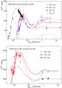 |
Fig. B.1 Total inelastic (reaction) cross-section for the quartet isotopes. The lines show our parametrisation (see text), the symbols are data. Top panel: reaction on H with data from Cairns et al. (1964); Hayakawa et al. (1964); Igo et al. (1967); Palevsky et al. (1967); Griffiths & Harbison (1969); Nicholls et al. (1972); Carlson et al. (1973); Sourkes et al. (1976); Ableev et al. (1977); Klem et al. (1977); Jaros et al. (1978); Velichko et al. (1982); Blinov et al. (1984, 1985); Abdullin et al. (1993); Glagolev et al. (1993); Webber (1997). Bottom panel: reaction on He with data from Koepke & Brown (1977); Jaros et al. (1978); Tanihata et al. (1985). |
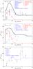 |
Fig. B.2 Inclusive production cross-sections of 3He (top), 2H (centre) and 3H (bottom) in 4He+H reaction. The data (see text for details) are from Tannenwald (1953); Innes (1957); Cairns et al. (1964); Rogers et al. (1969); Griffiths & Harbison (1969); Meyer (1972); Jung et al. (1973a); Aladashvill et al. (1981); Webber (1990b); Glagolev et al. (1993); Abdullin et al. (1994). |
The most accurate set of data (upward blue empty triangles) are from the experiments set up in ITEP and LHE JINR (Aladashvill et al. 1981; Glagolev et al. 1993; Abdullin et al. 1994; summarised in Blinov & Chadeyeva 2008). Their highest energy data point (Glagolev et al. 1993) is a conservative estimate because the more than, or equal to, six-prong reactions are not detailed (see Table 3 of Blinov & Chadeyeva 2008; and Table 4 of Glagolev et al. 1993). To take into account that possibility, we considered an error of a few mb in the plots of Fig. B.2. Let us consider each product of interest in turn.
3He production.
The stripping cross-section data (d and 3He in the final state) are well-fitted by Eq. (130) of Cucinotta et al. (1993). However, the Griffiths & Harbison (1969) and Jung et al. (1973a) values are ~ 30% below the other data. Indeed, for the latter (filled stars) the break-up cross-section is higher than other data, it may be that the end products are misreconstructed (in this or the other experiments). Nevertheless, the sum of the two – which is the one that matters – is consistent in all data. Note that we slightly modified the break-up cross-section provided by Cucinotta et al. (1993) to better fit the high-energy data points. For the latter, all data are consistent with each other, except for the high-precision ITEP data at 200 MeV/n.
2H production.
The stripping cross-section is the same as for 3He (d and 3He in the final state). The high-energy break-up cross-section data (LHE JINR and Webber 1990b) are inconsistent. We decided to rescale the Webber data to take into account the fact that in his preliminary account of the results (Webber 1990b), the total inelastic cross-section is smaller than that given in a later and updated study (Webber 1997). Still, the agreement between the two sets is not satisfactory. The other high-energy data point is the Innes (1957) experiment, and it suffers large uncertainties and maybe systematics (it is for n + 4He reaction, and the data point is provided by Meyer (1972) who relied on several assumptions to derive it). The ITEP/LHE JINR data being the best available, we replaced the formula for the 2H breakup of Cucinotta et al. (1993) by a form similar to that given for 3He, but we changed the parameters to fit the high-energy points.
3H production.
There is only break-up for the Cucinotta et al. (1993)3H production. The data broadly agree with each other, except for the Nicholls et al. (1972) point (open plus). Again, we adapted the Cucinotta et al. (1993) parametrisation to better fit the ITEP/LHE JINR data.
B.2.2. 3He + p → 2H (breakup) and p + p → 2H (fusion)
There are two other channels for producing 2H from light nucleus reactions, and they are shown in Fig. B.3 along with the data. The first one is from 3He (break-up and stripping). The CR flux of the latter is less abundant than the 4He flux. With a ratio of ~20% at 1 GeV/n (decreasing at higher energy) and similar production cross-sections (~30−40 mb), this is expected to contribute the same fraction at GeV/n energies, and then to become negligible ≳ 10 GeV/n. The second channel is the 2H coalescence from two protons. The cross-section is non-vanishing only for a very narrow energy range. Even if the cross-section is 10 times smaller than for the other channels, the fact that CR protons are ~10 times more numerous than 4He makes it a significant channel slightly below 1 GeV/n.
The fitting curves were taken from Meyer (1972), but we adapted the fit for the 3He+p channel to match the two high-energy ITEP/LHE JINR data points.
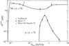 |
Fig. B.3 2H other production channels from the less abundant 3He and the peaked fusion pp reaction (the much smaller cross-section for the pp reaction compared to the 3Hep one is redeemed by a CR flux higher for p than for 3He). The data are from Griffiths & Harbison (1969); Meyer (1972); Blinov et al. (1986); Glagolev et al. (1993). |
B.2.3. Proj(A>4) + p → 2H, 3H, and 3He
For nuclear fragmentation cross-sections of heavier nuclei, the concepts of “strong” or “weak” factorisation relies on the fact that at sufficiently high energy, the branching of the various outgoing particles-production channels becomes independent of the target. This corresponds to the factorisation 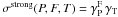 or
or 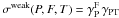 where σ(P,F,T) is the fragmentation cross-section for the projectile P incident upon the target T producing the fragment F. This is discussed, e.g., in Olson et al. (1983), who concluded that although strong factorisation is probably violated, weak factorisation seems exact (see also, e.g., Michel et al. 1995). The parametrisation proposed below takes advantage of this.
Several data exist for the production of light isotopes from nuclei A ≥ 12 on H (see Table B.1). The most complete sets of data in terms of energy coverage are for the projectiles C, N, and O ( ⟨ A ⟩ = 14), the group Mg, Al, and Si ( ⟨ A ⟩ = 26), and the group Fe and Ni ( ⟨ A ⟩ = 57). They are plotted in Fig. B.4 (top panels and bottom left panel). The solid lines correspond to an adjustment (by eye), rescaled from the  cross-section (because heavy projectiles do not give A = 3 fragments in the stripping process). Because
  , no distinction was made for the fit (2H data are scarce and do not influence the conclusions drawn from these three groups of nuclei). The following parametrisation
  (B.1)with
  (B.2)proves to fit the three groups of data well for energies greater than ~30 MeV/n. Thanks to the f(Ek/n,Aproj) factor, there is no other energy dependence in the
  factor, so that the latter can be determined from the data points at any energy. The bottom right panel of Fig. B.4 shows the measured mean value and dispersion14 as a function of A, from which we obtained:
 ![\appendix \setcounter{section}{2} \begin{eqnarray} \gamma_{\rm P}^{\het{}} &=& \gamma_{\rm P}^{\trit{}} = 1.3\, \left[ 1 + \left( \frac{A_{\rm P}}{25}\right)^{1.5}\right], \nonumber\\ \gamma_{\rm P}^{\deut{}} &=& 0.28\, A_{\rm P}^{1.2}. \label{eq:Nucp3} \end{eqnarray}](/articles/aa/full_html/2012/03/aa17927-11/aa17927-11-eq417.png) (B.3)The set of formulae (B.1), (B.2), and (B.3) completely define the Proj+p production cross-sections for the light fragments.
(B.3)The set of formulae (B.1), (B.2), and (B.3) completely define the Proj+p production cross-sections for the light fragments.
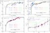 |
Fig. B.4 Proj(A>4) + p → 2H, 3H, and 3He cross-sections for Proj = C, N, O (top left), Proj = Mg, Al, Si (top right), and Proj = Fe, Ni (bottom left). The bottom right correspond to the |

B.3. Proj(A≥4) + 4He → 2H, 3H, and 3He
Data for T + 4He where the target T is heavier than p are scarce. In a compilation of Davis et al. (1995), the authors find that the 3He production scales as  (based on four data points with AT ≥ 7). This is the scaling we employed for the 3H and 2H production as well.
All Tables
All Figures
|
Fig. 1 Analysis of simulated interstellar (IS) data sets for the 3He/4He ratio (top panel) and the 4He flux times |
| In the text | |
|
Fig. 2 Marginalised posterior PDF for the transport and source parameters on the artificial data for Model II (the values for the input model are shown as thick vertical grey lines in each panel). The colour code and style correspond to the five “options” described in Sect. 3.2 (same as in Fig. 1). |
| In the text | |
|
Fig. 3 Fractional contributions to the propagated 2H fluxes (top panel), 3He fluxes (middle panel) and 4He fluxes (bottom panel) as a function of Ek/n from A > 4 CR parents. For 4He, the primary contribution is also considered. |
| In the text | |
|
Fig. 4 Left panels: demodulated interstellar 2H (top) and 3He (bottom) envelopes at 95% CIs times |
| In the text | |
|
Fig. B.1 Total inelastic (reaction) cross-section for the quartet isotopes. The lines show our parametrisation (see text), the symbols are data. Top panel: reaction on H with data from Cairns et al. (1964); Hayakawa et al. (1964); Igo et al. (1967); Palevsky et al. (1967); Griffiths & Harbison (1969); Nicholls et al. (1972); Carlson et al. (1973); Sourkes et al. (1976); Ableev et al. (1977); Klem et al. (1977); Jaros et al. (1978); Velichko et al. (1982); Blinov et al. (1984, 1985); Abdullin et al. (1993); Glagolev et al. (1993); Webber (1997). Bottom panel: reaction on He with data from Koepke & Brown (1977); Jaros et al. (1978); Tanihata et al. (1985). |
| In the text | |
|
Fig. B.2 Inclusive production cross-sections of 3He (top), 2H (centre) and 3H (bottom) in 4He+H reaction. The data (see text for details) are from Tannenwald (1953); Innes (1957); Cairns et al. (1964); Rogers et al. (1969); Griffiths & Harbison (1969); Meyer (1972); Jung et al. (1973a); Aladashvill et al. (1981); Webber (1990b); Glagolev et al. (1993); Abdullin et al. (1994). |
| In the text | |
|
Fig. B.3 2H other production channels from the less abundant 3He and the peaked fusion pp reaction (the much smaller cross-section for the pp reaction compared to the 3Hep one is redeemed by a CR flux higher for p than for 3He). The data are from Griffiths & Harbison (1969); Meyer (1972); Blinov et al. (1986); Glagolev et al. (1993). |
| In the text | |
|
Fig. B.4 Proj(A>4) + p → 2H, 3H, and 3He cross-sections for Proj = C, N, O (top left), Proj = Mg, Al, Si (top right), and Proj = Fe, Ni (bottom left). The bottom right correspond to the |
| In the text | |
Current usage metrics show cumulative count of Article Views (full-text article views including HTML views, PDF and ePub downloads, according to the available data) and Abstracts Views on Vision4Press platform.
Data correspond to usage on the plateform after 2015. The current usage metrics is available 48-96 hours after online publication and is updated daily on week days.
Initial download of the metrics may take a while.