© ESO, 2012

1. Introduction

Molecular lines, such as C₂ and MgH lines, which are observed in the so-called second solar spectrum, show a significant amount of linear polarization, which increases as one approaches the solar limb. This polarization is due to scattering processes and is further modified by magnetic field and depolarizing collisions. It is used as a tool for magnetic field diagnostic via the Hanle effect and differential Hanle effect on lines with different magnetic sensitivity (Faurobert & Arnaud 2003; Berdyugina & Fluri 2004; Bommier et al. 2006; Shapiro et al. 2011). Plane-parallel geometry is sufficient to model outgoing radiation for observations made on the solar disk. However, Faurobert & Arnaud (2002) measured polarization above the solar limb in the spectral range from 515.60 nm to 516.20 nm, where molecular lines of C₂ and MgH are seen in emission, and found a much greater degree of linear polarization (a few percent) than what is observed on the solar disk. To interpret observations performed close to and above the limb, it appears necessary to take the sphericity of the solar atmosphere into account. There are several reasons this effect should affect the degree of scattering polarization, the most important one being that by looking at the solar limb, one looks through a longer optical path than expected from plane-parallel geometry, while also looking at a more dilute medium, which is dominated by scattering processes. In this paper we revisit the modeling of scattering polarization in C₂ and MgH molecular lines, taking sphericity of the solar atmosphere into account. The solar atmosphere is modeled as a one-dimensional, spherically symmetric medium.

Stenflo & Stenholm (1976) computed scattering polarization in chromospheric UV emission lines in spherical geometry using an along-the-ray analysis and representing the line-forming region as a thin slab illuminated by an unpolarized continuum radiation. In this work we model the 515.98 nm MgH and the 515.96 nm C₂ polarized line formation self consistently and compare the results for plane-parallel and spherical geometries. We use FALC and FALX solar models (Fontenla et al. 1993; Avrett 1995) in order to inspect the effects of different temperature distributions on line and continuum polarization. FALC is the standard model for the average quiet Sun, while FALX is a model with a cool chromosphere that accounts for the observed intensity in the infrared CO lines. As we see in the following, the molecular lines of MgH and C₂ observed at the solar limb and slightly above the limb are formed in the minimum temperature region between the photosphere and the chromosphere, where the two models differ. As the temperature in the chromosphere is probably quite inhomogeneous, 2D or 3D models would probably provide a more realistic view of the formation of molecular lines at the solar limb, but this is beyond the scope of this paper.

We solve the polarized radiative transfer problem for the lines and continuum background radiation using a two-level formulation of the line source function, without any approximation of the optical thickness of the line-forming region. Elastic and inelastic collisions play an important role in the scattering mechanism but their rates are presently poorly known for the molecular lines we are considering. Before modeling the line in spherical geometry, we therefore first use disk observations reported in the Second Solar Spectrum Atlas by Gandorfer (2000) in several MgH and C₂ lines in order to estimate these collision cross-sections. We implement the differential Hanle effect method first applied by Bommier et al. (2006) to MgH lines, to derive C₂ elastic collision cross-sections. In Sect. 2 we describe the polarized transfer problem and comment on our method of solving it. In Sect. 3 we list and explain how we compute necessary molecular data and collision cross-sections. Results for the linear polarization in spherical geometry, in the absence and in the presence of Hanle effect, are presented in Sect. 4.

2. Radiative transfer

2.1. Transfer equation

In the absence of a magnetic field (or in the case of a microturbulent, i.e. weak and unresolved, magnetic field) for an axially-symmetric radiation field only two components of the radiation field Stokes vector are different from zero so we can write Π= (I,Q)^† and cast the radiative transfer equation along the ray in the following form, 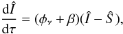$\frac{\mathrm{d}\mathit{Î}}{\mathrm{d}\mathit{\tau }}\mathrm{=}\mathrm{(}{\mathit{\phi }}_{\mathit{\nu }}\mathrm{+}\mathit{\beta }\mathrm{)}\mathrm{(}\mathit{Î}\mathrm{-}\mathit{Ŝ}\mathrm{)}\mathit{,}$(1)where Ŝ is the source function vector, τ line-integrated optical depth along the ray, φ_ν the absorbtion profile, and β the continuum-to-line opacity ratio. We follow the sign convention for Q introduced by Chandrasekhar (1960), where a linear polarization parallel to the solar limb is negative. We see that this is indeed the most common situation for resonance line polarization observed at the solar limb, so in the following, all the figures show the opposite of Q/I. The total source function vector can be written as a weighted sum of the line and continuum source functions: 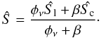$\mathit{Ŝ}\mathrm{=}\frac{{\mathit{\phi }}_{\mathit{\nu }}\widehat{{\mathit{S}}_{\mathrm{l}}}\mathrm{+}\mathit{\beta }\widehat{{\mathit{S}}_{\mathrm{c}}}}{{\mathit{\phi }}_{\mathit{\nu }}\mathrm{+}\mathit{\beta }}\mathrm{·}$(2)Dealing with weak molecular lines, it is reasonable to assume complete redistribution. We also assume here that the line may be modeled with a two-level formalism, so the line source vector is given by 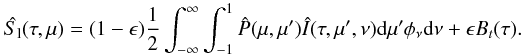$\widehat{{\mathit{S}}_{\mathrm{l}}}\mathrm{\left(}\mathit{\tau ,\mu }\mathrm{\right)}\mathrm{=}\mathrm{(}\mathrm{1}\mathrm{-}\mathit{ϵ}\mathrm{)}\frac{\mathrm{1}}{\mathrm{2}}{\mathrm{\int }}_{\mathrm{-}\mathrm{\infty }}^{\mathrm{\infty }}{\mathrm{\int }}_{-1}^{\mathrm{1}}\mathit{P̂}\mathrm{\left(}\mathit{\mu ,}{\mathit{\mu }}^{\mathrm{\prime }}\mathrm{\right)}\mathit{Î}\mathrm{\left(}\mathit{\tau ,}{\mathit{\mu }}^{\mathrm{\prime }}\mathit{,\nu }\mathrm{\right)}\mathrm{d}{\mathit{\mu }}^{\mathrm{\prime }}{\mathit{\phi }}_{\mathit{\nu }}\mathrm{d}\mathit{\nu }\mathrm{+}\mathit{ϵ}{\mathit{B}}_{\mathit{t}}\mathrm{\left(}\mathit{\tau }\mathrm{\right)}\mathit{.}$(3)The coefficient ϵ is the branching ratio for collisional destruction of line photons, i.e. ϵ = C_ul/(C_ul + A_ul), where C_ul denotes the inelastic collision rate, A_ul the Einstein coefficient for spontaneous radiative de-excitation in the line, B_t the Planck function, and the scattering phase matrix. In the nonmagnetic case or in the presence of a microturbulent weak magnetic field, it is given by 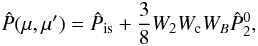$\mathit{P̂}\mathrm{\left(}\mathit{\mu ,}{\mathit{\mu }}^{\mathrm{\prime }}\mathrm{\right)}\mathrm{=}\mathit{P̂}\mathrm{is}\mathrm{+}\frac{\mathrm{3}}{\mathrm{8}}{\mathit{W}}_{\mathrm{2}}{\mathit{W}}_{\mathrm{c}}{\mathit{W}}_{\mathit{B}}\mathit{P̂}\begin{array}{}\mathrm{0}\\ \mathrm{2}\end{array}\mathit{,}$(4)where μ and μ′ denote the cosines of the heliocentric angles of the outgoing and ingoing radiation propagation direction, respectively and is the isotropic matrix. And $\mathit{P̂}\begin{array}{}\mathrm{0}\\ \mathrm{2}\end{array}$, the anisotropic part of the phase matrix, is given by 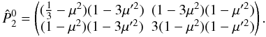$\mathit{P̂}\begin{array}{}\mathrm{0}\\ \mathrm{2}\end{array}\mathrm{=}\left(\begin{array}{c}\\ \mathrm{(}\frac{\mathrm{1}}{\mathrm{3}}\mathrm{-}{\mathit{\mu }}^{\mathrm{2}}\mathrm{)}\mathrm{(}\mathrm{1}\mathrm{-}\mathrm{3}{\mathit{\mu }}^{\mathrm{\prime }\mathrm{2}}\mathrm{)}& \mathrm{(}\mathrm{1}\mathrm{-}\mathrm{3}{\mathit{\mu }}^{\mathrm{2}}\mathrm{)}\mathrm{(}\mathrm{1}\mathrm{-}{\mathit{\mu }}^{\mathrm{\prime }\mathrm{2}}\mathrm{)}\\ \mathrm{(}\mathrm{1}\mathrm{-}{\mathit{\mu }}^{\mathrm{2}}\mathrm{)}\mathrm{(}\mathrm{1}\mathrm{-}\mathrm{3}{\mathit{\mu }}^{\mathrm{\prime }\mathrm{2}}\mathrm{)}& \mathrm{3}\mathrm{(}\mathrm{1}\mathrm{-}{\mathit{\mu }}^{\mathrm{2}}\mathrm{)}\mathrm{(}\mathrm{1}\mathrm{-}{\mathit{\mu }}^{\mathrm{\prime }\mathrm{2}}\mathrm{)}\end{array}\right)\mathit{.}$(5)Here, W₂ is the intrinsic polarizability, W_c the collisional depolarization coefficient, and W_B the Hanle depolarization coefficient. Parameter W_c is given by 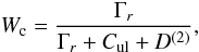${\mathit{W}}_{\mathrm{c}}\mathrm{=}\frac{{\mathrm{\Gamma }}_{\mathit{r}}}{{\mathrm{\Gamma }}_{\mathit{r}}\mathrm{+}{\mathit{C}}_{\mathrm{ul}}\mathrm{+}{\mathit{D}}^{\mathrm{\left(}\mathrm{2}\mathrm{\right)}}}\mathit{,}$(6)where Γ_r is line radiative damping and D⁽²⁾ the depolarizing collision rate. In the presence of a weak isotropic microturbulent magnetic field, the Hanle depolarization coefficient depends on the so-called Hanle parameter Γ_H. It has the form, ${\mathit{W}}_{\mathit{B}}\mathrm{=}\mathrm{1}\mathrm{-}\frac{\mathrm{2}}{\mathrm{5}}\left[\frac{{\mathrm{\Gamma }}_{\mathrm{H}}^{\mathrm{2}}}{\mathrm{1}\mathrm{+}{\mathrm{\Gamma }}_{\mathrm{H}}^{\mathrm{2}}}\mathrm{+}\frac{\mathrm{4}{\mathrm{\Gamma }}_{\mathrm{H}}^{\mathrm{2}}}{\mathrm{1}\mathrm{+}\mathrm{4}{\mathrm{\Gamma }}_{\mathrm{H}}^{\mathrm{2}}}\right]\mathrm{·}$(7)The Hanle parameter depends on the upper level Landé factor g, the magnetic field strength B, and the upper level alignment inverse lifetime, ${\mathrm{\Gamma }}_{\mathrm{H}}\mathrm{=}\mathrm{0.88}\frac{\mathit{gB}}{{\mathrm{\Gamma }}_{\mathit{r}}\mathrm{+}{\mathit{C}}_{\mathrm{ul}}\mathrm{+}{\mathit{D}}^{\mathrm{\left(}\mathrm{2}\mathrm{\right)}}}\mathit{,}$(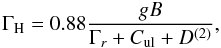8)where the magnetic field strength is given in Gauss and D⁽²⁾, C_ul, and Γ_r are all expressed in units of 10⁷ s^-1. We see in the following that the inelastic collision rate C_ul is much lower than the elastic collision rate D⁽²⁾.

In the continuum, the emissivity may be cast into two terms: i) one thermal term due to photoionization and free-free mechanisms, which is proportional to the Planck function and does not give rise to continuum polarization; and ii) one scattering term due to Rayleigh and Thomson scattering mechanisms, which gives rise to linear polarization with a Rayleigh phase matrix in the form $\mathit{P̂}\mathrm{=}\mathit{P̂}{}_{\mathrm{is}}\mathrm{+}\frac{\mathrm{3}}{\mathrm{8}}\mathit{P̂}\begin{array}{}\mathrm{0}\\ \mathrm{2}\end{array}$. The continuum radiation is not affected by collisional and Hanle depolarization, the source function is thus given by 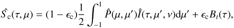$\widehat{{\mathit{S}}_{\mathrm{c}}}\mathrm{\left(}\mathit{\tau ,\mu }\mathrm{\right)}\mathrm{=}\mathrm{(}\mathrm{1}\mathrm{-}{\mathit{ϵ}}_{\mathrm{c}}\mathrm{)}\frac{\mathrm{1}}{\mathrm{2}}{\mathrm{\int }}_{-1}^{\mathrm{1}}\mathit{P̂}\mathrm{\left(}\mathit{\mu ,}{\mathit{\mu }}^{\mathrm{\prime }}\mathrm{\right)}\mathit{Î}\mathrm{\left(}\mathit{\tau ,}{\mathit{\mu }}^{\mathrm{\prime }}\mathit{,\nu }\mathrm{\right)}\mathrm{d}{\mathit{\mu }}^{\mathrm{\prime }}\mathrm{+}{\mathit{ϵ}}_{\mathrm{c}}{\mathit{B}}_{\mathit{t}}\mathrm{\left(}\mathit{\tau }\mathrm{\right)}\mathit{,}$(9)with ϵ_c = χ_abs/(χ_sc + χ_abs), where χ_abs and χ_sc respectively denote the absorption and scattering continuum opacities that we compute with the Uppsala package, using FALC and FALX quiet Sun models. The main absorbing mechanism in the continuum in our wavelength range is the photoionization of H ⁻ , but we also take the possible photoionization and free-free processes for hydrogen and helium atoms into account. The dominant scattering mechanisms in the spectral domain we are considering are Thomson scattering on free electrons and Rayleigh scattering on hydrogen atoms, which both have polarizability unity (Stenflo 2005). We stress that we do not introduce any effective continuum polarizability since we solve the full polarized transfer equation in both the line and the continuum as written in Eqs. (2) to (9). However, the branching ratio 1 − ϵ_c in the continuum source function, in a way, is similar to the effective polarizability introduced in Stenflo (2005).

The approximation of two-level atom model is also a matter of particular interest. While this is a good approximation for MgH transition, there are some indications that for C₂ there could be some important contributions from other levels. The upper level could, for example, be excited by transitions from different rotational and vibrational levels. For weak lines like those we are considering here, one may take this coupling into account by using effective intrinsic polarizabilities in an equivalent two-level formalism, as suggested by Landi Degl’Innocenti (2006). However, our main goal here is to compare computations in two geometries and to get order-of-magnitude line polarization in regions close to the solar limb. We therefore stick to the two-level approximation and use the intrinsic line polarizabilities given in Berdyugina et al. (2002). In this two-level model, for the weak lines we consider here, the lower level population is almost not affected by radiative transitions in the line, so that LTE population of the lower level may be safely used for computing the line optical depth (see also Bommier et al. 2006).

2.2. Solving the radiative transfer problem in spherical geometry

First, we notice that, since the geometrical thickness of the solar atmosphere is negligible compared to the solar radius, sphericity effects will be important only for very inclined lines of sight. Since they play a negligible role in the angle-averaged intensity, level populations and line absorption coefficients may be computed in plane-parallel geometry and the source function for the intensity is weakly affected by sphericity effects. To solve the coupled system of Eqs. (1)–(4) we proceed in two steps. In the first step, we solve the scalar radiative transfer problem for the intensity, while neglecting polarization and assuming a plane-parallel geometry. This is achieved by the “forth-and-back” implicit lambda iteration (FBILI) method (Atanacković-Vukmanović et al. 1997). It is an iterative method, similar in a way to ALI iterative scheme. It makes use of a local approximate operator, but uses a two-point representation of source function in formal solution, as well as iteration factors to handle nonlocal parts in formal solution of the radiative transfer equation. This results in a very fast rate of convergence, even without any additional acceleration. After obtaining self-consistent values for the scalar source function, we consider polarization and spherical geometry. We start with the assumption Ŝ = (S,0)^†, where S is the scalar source function computed in the previous step, and proceed iteratively, solving in turn Eq. (1) and computing the source functions according to Eqs. (3), (4), until convergence. This iterative solution is in essence an ordinary Λ iteration for the polarization, which converges relatively fast, in fewer than 10 iterations.

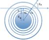Fig. 1 Geometry of radiative transfer with sphericity taken into account. The line of sight with impact parameter rk is located at height h above the solar limb, i.e. rk = R⊙ + h. At depth point rd, the heliocentric angle of the line of sight is θd.

When solving the radiative transfer equation in spherical geometry, we avoid the partial differential equation form by using the simpler, “along-the-ray” approach, as described, for example, by Avrett & Loeser (1984). We compute the scattering integral at each depth point with an angular grid containing both “core rays” and “surface rays”. Core rays are rays that intersect the solar disk, whereas surface rays only pass through the atmospheric layers. The lower boundary condition for core rays is derived from the diffusion approximation, whereas for surface-rays, we prescribe a condition of symmetry of the radiation field at the central depth point. To get a fine angular mesh at the surface, we use 40 core rays and as many surface rays as depth points in the atmospheric model.

In spherical geometry, the heliocentric angle varies along the line of sight. This is sketched in Fig. 1, where we show a line of sight at distance h from the limb, defined by its impact parameter r_k = R_⊙ + h with respect to disk center, R_⊙ denotes the solar radius (h is a negative quantity for observations performed inside the solar limb). The heliocentric angle of the line of sight at depth point r_d (defined with respect to disk center) is such that $\mathit{\mu }\mathrm{=}\sqrt{\mathrm{1}\mathrm{-}\mathrm{(}{\mathit{r}}_{\mathit{k}}\mathit{/}{\mathit{r}}_{\mathrm{d}}{\mathrm{)}}^{\mathrm{2}}}\mathit{.}$(10)The variable μ is therefore not well suited to comparing results in plane-parallel and spherical geometries. A more suitable quantity is the line-of-sight limb distance δ. It is given in arcsec by $\mathit{\delta }\mathrm{=}\frac{\mathit{h}}{{\mathit{R}}_{\mathrm{\odot }}}\mathrm{\times }{\mathrm{960}}^{\mathrm{\prime \prime }}\mathit{.}$(11)We define the limb as the point where the continuum limb darkening curve I(δ) changes its behavior from concave to convex. From our computations we find that the solar limb altitude is 325 km above the continuum formation height for both FALC and FALX models. This point is also used to define the solar radius.

3. Molecular data

3.1. Molecular number density and line absorption coefficient

To construct the optical depth scales we must first find the molecular number densities and compute lower state populations. The MgH line belongs to the Q band of the A²Π − X²Σ ⁺ (0,0) transition, with J = 16 where J is the rotational lower level quantum number and the C₂ line belongs to the P3 band of the d³Π_g − a³Π_u transition with J = 26. The molecular number densities obey the equilibrium equation, given by, say Berdyugina et al. (2003): $\frac{\mathit{n}\mathrm{\left(}\mathit{A}\mathrm{\right)}\mathit{n}\mathrm{\left(}\mathit{B}\mathrm{\right)}}{\mathit{n}\mathrm{\left(}\mathit{AB}\mathrm{\right)}}\mathrm{=}{\mathit{K}}_{\mathrm{AB}}\mathit{,}$(12)where n(AB),n(A), and n(B) are, respectively, the molecule number density and the constituting atom densities, and K_AB is the equilibrium constant.

In general, equilibrium constant depends on temperature, partition functions of the given molecule and constituting atoms and on the dissociation energy of the molecule. Convenient polynomial expressions for equilibrium constants and molecule partition functions are given by Sauval & Tatum (1984). In general, to obtain exact molecular number densities, one should take all molecules and all constituting atoms into account and solve a system of non-linear equations as explained by Berdyugina et al. (2003). However, owing to the relatively high temperatures, molecular densities are low, so when computing the MgH density, we may approximate n(Mg) with the total number density of magnesium derived from its abundance relative to hydrogen. The situation is a bit more complicated when it comes to computing the C₂ density, due to the presence of CO whose number density may be a significant fraction of the total number density of carbon, especially in cool regions of the atmosphere, so we consider both CO and C₂ molecules in equilibrium with atomic carbon and oxygen. Number densities follow from a system of four nonlinear algebraic equations. For element abundances we use A_Mg = 7.6, A_C = 8.43, and A_O = 8.69 for magnesium, carbon and oxygen respectively, as suggested by Grevesse et al. (2010). Then to compute the line opacity, we assume that for weak molecular lines the population of the a lower level of the transition follows from ${\mathit{n}}_{\mathrm{l}}\mathrm{=}{\mathit{n}}_{\mathrm{total}}\frac{\mathrm{2}\mathit{J}\mathrm{+}\mathrm{1}}{\mathit{Q}}\exp \mathrm{(}\mathrm{-}{\mathit{E}}_{\mathrm{ex}}\mathit{/}\mathit{kT}\mathrm{)}\mathit{,}$(13)where n_total is the total molecular number density, J the lower level rotational quantum number, Q the molecular partition function, and E_ex the excitation energy, which can be computed as ${\mathit{E}}_{\mathrm{ex}}\mathrm{=}\mathit{BJ}\mathrm{(}\mathit{J}\mathrm{+}\mathrm{1}\mathrm{)}\mathrm{+}{\mathit{E}}_{\mathrm{vib}}^{\mathrm{0}}$ where B is Herzberg’s constant, B = 5.735   cm^-1 for MgH and B = 1.632   cm^-1 for C₂. Here, ${\mathit{E}}_{\mathrm{vib}}^{\mathrm{0}}$ is the vibrational energy of lower level of the transition. Values for B and E_vib are computed as given in Herzberg (1950). The line-integrated opacity, neglecting stimulated emission, is given by $\mathit{\chi }\mathrm{=}\frac{{\mathit{n}}_{\mathrm{l}}\mathit{h\nu }}{\mathrm{4}\mathit{\pi }}{\mathit{B}}_{\mathrm{lu}}\mathit{,}$(14)where B_lu is Einstein coefficient of radiative excitation, which follows from the coefficient of spontaneous emission A_ul.

3.2. Collision rates

In the case of molecular lines, elastic collisions mainly come from neutral hydrogen atoms, and both electrons and neutral hydrogen contribute to inelastic collisions (Shapiro et al. 2011). Unfortunately, accurate collision rates are presently not available for the molecular lines we are considering here.

3.2.1. Inelastic collisions

The issue of inelastic collisions rates has been previously discussed by Asensio Ramos & Trujillo Bueno (2005) and Bommier et al. (2006). In order to get order-of-magnitude values for the collisional rates we use the following approach. As in Shapiro et al. (2011), we write ${\mathit{C}}_{\mathrm{ul}}\mathrm{=}\mathit{\alpha }\hspace{0.17em}{\mathit{n}}_{\mathrm{H}}{\mathit{T}}^{\mathrm{0.3}}\mathit{.}$(15)We then set α as a free parameter and fit our computed line equivalent width ratio to the one observed by Gandorfer (2000) at δ =  −9′′ inside the solar limb (with 9′′ the value given in the atlas, ch. 2, p. 11). The corresponding heliocentric angle θ is such that sinθ = 1 + δ/R_⊙ = 0.9906, and μ = cos(θ) ≈ 0.137, if we take for the solar radius, the average value R_⊙ = 960′′. We notice that the value μ = 0.1 that is adopted in the atlas would give sinθ = 0.9950. As the apparent angular radius of the Sun varies between 944′′ and 976′′, the cosine of the heliocentric angle at the same δ =  −9′′ varies between μ = 0.136 and μ = 0.138. The value adopted in Gandorfer’s Atlas thus appears to be inconsistent with δ =  −9′′. Moreover, to increase the signal-to-noise ratio, the data presented in the Atlas was obtained by integrating the signal along a 180′′-long slit, parallel to the solar limb. If the center of the slit is 9′′ inside the limb, the slit edges are at 4.7′′ inside the limb, which corresponds to μ = 0.1. As scattering polarization shows nonlinear sharp variations with limb distance when approaching the limb, one should make a proper averaging of the computed profiles on the μ-interval 0.10–0.14, when comparing model calculations with the Atlas data. One also has to keep in mind that guiding problems and seeing effect during the observations may lead to fluctuations of δ on the order of one arcsec or more, which may integrate in the signal regions located quite close to the limb, where a plane-parallel model is not valid anymore, as we see in the following.

At that range of observing angles, the line optical depth is larger by an order of magnitude then its value at disk center, and scattering effects do modify the intensity at line center. In Fig. 2 we show the line shapes of our selected MgH and C₂ lines, integrated along the slit for different values of α. A good fit to the observations is obtained by using α = 0.8 × 10^-12   cm³   s^-1   K^-0.3 for the MgH line and α = 1.3 × 10^-12   cm³   s^-1   K^-0.3 for the C₂ line. This leads to ϵ ≃ 0.02 for MgH and ϵ ≃ 0.08 for C₂ in the line-forming region (h ≈ 200   km). These values are somewhat higher than what is assumed in Bommier et al. (2006), but as already pointed out in her paper, as long as the value of ϵ is significantly less then unity, they will lead to approximately the same degree of linear polarization. We also show (Fig. 2c) computed lines plotted along with the observations from the Atlas to illustrate the quality of the fit. The epsilon values given above allows us to fit the line equivalent widths, but to fit the line profiles we have to account for a macroturbulent velocity field of 1.9 km s^-1. This also affects the computed linear polarization profile. Therefore, it is important to account for macroturbulent velocity if one wants to compare line and polarization profiles with observed ones. For details on including the macrotubulent velocity see also Faurobert et al. (2001). We stress that this is an approximate way of estimating inelastic collisional rates. In order to get more reliable values, more observations are needed at various limb distances. We notice that the line profile at disk center is very weakly sensitive to the value of the inelastic collision rate. The reason is that, as the lines are weak, their intensity at disk center is very close to the continuum intensity, which is very close to the Planck function at the line forming height, so the scattering integral in the line source function is very close to the Planck function, too (and the line polarization vanishes). In that situation, the total line source function is close to the Planck function, regardless of the value of the branching ratio 1 − ϵ.

In Fig. 3 we show the dependence of the line polarization rates on the coefficient α for observations performed on the limb and above the limb. We notice that the line polarization observed inside the solar limb is relatively more sensitive to the value of α than off-limb observations. This is to be expected since the density sharply decreases with the altitude in the solar atmosphere. The variations in ϵ with height corresponding to our best fit for α, together with the number densities of the molecular line lower levels, are shown in Fig. 4 for the MgH and the C₂ line, respectively, in the case of the FALC model.

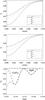Fig. 2 C2 and MgH line profiles computed at 9′′ inside the solar limb with the FALC model, for different values of the parameter α defined in Eq. (15). Upper panel: MgH line, α values result in ϵ = 0.0025, 0.024, 0.2, 0.71 at 200 km above the base of the photosphere. Middle panel: C2 line. Corresponding values of ϵ = 0.007, 0.065, 0.41, 0.87. Lower panel: computed profiles for best-fitting values of α parameter(dashed line) compared with the observations from the atlas (full line).

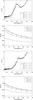Fig. 3 C2 and MgH line polarization rates computed with the FALC model, for different values of the parameter α defined in Eq. (15). Upper two panels: MgH line; lower two panels: C2 line.

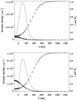Fig. 4 Upper panel: height variations in the lower level population of the MgH line in logarithmic scale (full line), probability of line photon collisional destruction, ϵ in units of 10-2 (asterisks), and collisional depolarization coefficient Wc (squares), computed with the FALC quiet Sun model. Bottom panel: same quantities for the C2 line.

3.2.2. Elastic collisions and differential Hanle effect

Elastic depolarizing collisions affect the outgoing polarization through the coefficient W_c (see Eq. (6)) in the scattering phase matrix, but also modify the value of the Hanle parameter Γ_H (see Eq. (8)). The rate of elastic collisions that destroy the alignment between Zeeman sublevels, D⁽²⁾, depends on the number density of neutral hydrogen in the form ${\mathit{D}}^{\mathrm{\left(}\mathrm{2}\mathrm{\right)}}\mathrm{=}{\mathit{\alpha }}^{\mathrm{\left(}\mathrm{2}\mathrm{\right)}}{\mathit{n}}_{\mathrm{H}}\mathit{.}$(16)In Eq. (16) we have included the weak temperature variations in D⁽²⁾ into the coefficient α⁽²⁾, as in Bommier et al. (2006) where its value is estimated to be α⁽²⁾ = (1.20 ± 0.21) × 10^-9 cm³ s^-1, for MgH lines in the temperature range of the upper solar photosphere. This estimate was obtained by a differential Hanle effect procedure, as described by Bommier et al. (2006). One of its remarkable advantages is that it allows us to determine both the elastic depolarizing collision rate and the mean strength of the turbulent magnetic field.

We now recall the main steps of the method and apply it to the C₂ lines. We consider two weak lines belonging to the same band, with the same radiative damping Γ_R but different Landé factors g_1,2. For weak lines we may neglect differential radiative transfer effects and simply write the ratio of their polarization rates in the form $\mathit{R}\mathrm{=}\frac{{\mathit{W}}_{\mathit{B}}^{\mathrm{\left(}\mathrm{1}\mathrm{\right)}}{\mathit{W}}_{\mathrm{2}}^{\mathrm{\left(}\mathrm{1}\mathrm{\right)}}{\mathit{W}}_{\mathit{C}}^{\mathrm{\left(}\mathrm{1}\mathrm{\right)}}}{{\mathit{W}}_{\mathit{B}}^{\mathrm{\left(}\mathrm{2}\mathrm{\right)}}{\mathit{W}}_{\mathrm{2}}^{\mathrm{\left(}\mathrm{2}\mathrm{\right)}}{\mathit{W}}_{\mathit{C}}^{\mathrm{\left(}\mathrm{2}\mathrm{\right)}}}\mathrm{·}$(17)We also assume then that their depolarizing collision rates are identical. Their Hanle parameters ${\mathrm{\Gamma }}_{\mathrm{H}}^{\mathrm{1}\mathit{,}\mathrm{2}}$ are thus simply related by ${\mathrm{\Gamma }}_{\mathrm{H}}^{\mathrm{\left(}\mathrm{1}\mathrm{\right)}}\mathrm{=}\mathrm{(}{\mathit{g}}_{\mathrm{1}}\mathit{/}{\mathit{g}}_{\mathrm{2}}\mathrm{)}{\mathrm{\Gamma }}_{\mathrm{H}}^{\mathrm{\left(}\mathrm{2}\mathrm{\right)}}$, and ${\mathit{W}}_{\mathit{C}}^{\mathrm{\left(}\mathrm{1}\mathrm{\right)}}\mathrm{=}{\mathit{W}}_{\mathit{C}}^{\mathrm{\left(}\mathrm{2}\mathrm{\right)}}$. Using Eq. (8) for W_B, and the relationship between ${\mathrm{\Gamma }}_{\mathrm{H}}^{\mathrm{\left(}\mathrm{1}\mathrm{\right)}}$ and ${\mathrm{\Gamma }}_{\mathrm{H}}^{\mathrm{\left(}\mathrm{2}\mathrm{\right)}}$, we get $\frac{\mathit{f}\mathrm{\left(}\mathit{x}\mathrm{\right)}}{\mathit{g}\mathrm{\left(}\mathit{x}\mathrm{\right)}}\mathrm{=}\mathit{R}\frac{{\mathit{W}}_{\mathrm{2}}^{\mathrm{\left(}\mathrm{2}\mathrm{\right)}}}{{\mathit{W}}_{\mathrm{2}}^{\mathrm{\left(}\mathrm{1}\mathrm{\right)}}}\mathit{,}$(18)where $\mathit{f}\mathrm{\left(}\mathit{x}\mathrm{\right)}\mathrm{=}\left(\mathrm{1}\mathrm{-}\frac{\mathrm{2}}{\mathrm{5}}\left[\frac{\mathrm{1}}{\mathrm{1}\mathrm{+}\mathrm{(}{\mathit{g}}_{\mathrm{2}}\mathit{/}{\mathit{g}}_{\mathrm{1}}{\mathrm{)}}^{\mathrm{2}}{\mathit{x}}^{\mathrm{2}}}\mathrm{+}\frac{\mathrm{4}}{\mathrm{4}\mathrm{+}\mathrm{(}{\mathit{g}}_{\mathrm{2}}\mathit{/}{\mathit{g}}_{\mathrm{1}}{\mathrm{)}}^{\mathrm{2}}{\mathit{x}}^{\mathrm{2}}}\right]\right)\mathit{,}$(19)and$\mathit{g}\mathrm{\left(}\mathit{x}\mathrm{\right)}\mathrm{=}\left(\mathrm{1}\mathrm{-}\frac{\mathrm{2}}{\mathrm{5}}\left[\frac{\mathrm{1}}{\mathrm{1}\mathrm{+}{\mathit{x}}^{\mathrm{2}}}\mathrm{+}\frac{\mathrm{4}}{\mathrm{4}\mathrm{+}{\mathit{x}}^{\mathrm{2}}}\right]\right)\mathit{,}$(20)where $\mathit{x}\mathrm{=}\mathrm{1}\mathit{/}{\mathrm{\Gamma }}_{\mathrm{H}}^{\mathrm{\left(}\mathrm{2}\mathrm{\right)}}$ and R is ratio of line polarization profiles maxima, with its value directly derived from observations. The solution of Eq. (18) gives the value of ${\mathrm{\Gamma }}_{\mathrm{H}}^{\mathrm{\left(}\mathrm{2}\mathrm{\right)}}$, we then derive ${\mathrm{\Gamma }}_{\mathrm{H}}^{\mathrm{\left(}\mathrm{1}\mathrm{\right)}}$. It is important to stress that, by using similar enough weak lines, this first step does not involve any radiative transfer calculations.

The method described above is straightforward for unblended and well-resolved lines. However, C₂ lines are often blended and sometimes unresolved. In the C₂ spectrum one finds blended P1(J + 1) and P2(J) lines and the P3(J − 1) line very close to them. But after modification, the scheme described above can still be applied. We will present a detailed analysis of differential Hanle effect procedure applied to C₂ lines in a separate paper. We only report here the main result regarding the depolarizing collisions rates that we use in the following. We applied this analysis to four C₂ triplets of Gandorfer’s atlas, which are presented in Table 1, with their Landé factors and intrinsic polarizabilities. Averaging the results we get Γ_H/g_J = 6 ± 2.

Solving separately the NLTE polarized radiative transfer problem in each line, with known values of the Hanle parameter, allows the elastic collision rate to be determined, which is still unknown and which appears in the depolarizing coefficient W_c. We find α⁽²⁾ for the C₂ molecule to be around 1.7 × 10^-9 cm³ s^-1, which is similar to the value obtained by Bommier et al. (2006) for the MgH molecule. This was expected from order-of-magnitude estimates (Bommier, priv. comm.).

4. Results and discussion

4.1. Optical paths and line optical depth

Figure 4 shows the height variations of the lower level population for the MgH and C₂ lines computed with FALC quiet Sun model. We see that both molecules are mostly concentrated in a 200 km wide slab located about 100 km above the base of the photosphere, defined as the level where the continuum optical depth along the radial direction at λ = 500 nm is unity. We notice that the molecular slab is located very close to the solar visible limb and that the number density of C₂ is significantly higher than that of MgH. For the FALC model, we find that the MgH line center optical thickness, measured along the radial direction, is 0.14 at the base of the photosphere. This is in good agreement with the computation of Bommier et al. (2006), where the difference corresponds exactly to different lower level statistical weights. (Bommier computes line integrated optical thickness of 0.08 for MgH line with J = 9.) The C₂ line is thicker, its optical thickness along the radial direction is larger by a factor of 2 (≈0.3). This agrees with results of Faurobert & Arnaud (2003) and Berdyugina & Fluri (2004), who find line center optical depth of C₂ line forming layer to be around 0.1. Radial optical depths computed with the FALX model are very similar, except in the region of the temperature minimum around z = 500 km, where molecular densities are higher thanks to lower temperatures in the FALX model. We now analyze the behavior of the line optical depths measured along the line-of-sight.

Figure 5 shows the variations in the line-of-sight optical depth as a function of limb distance for both the MgH and C₂ lines and the FALC model. We compared the results obtained in plane-parallel and spherical geometries for lines of sight close to the limb. There is little difference between both geometries for lines of sight inside the limb when the limb-distance is greater than 5 arcsec, but they differ significantly at smaller limb distances. An important thing to keep in mind is that, in spherical geometry, the optical path does not scale with observing direction as simply as Δτ_los = Δτ/μ (see Fig. 5). It shows a sharp maximum, for both lines, at δ ≃  −0.3′′. This value corresponds to the lines of sight that go through the molecular layer. Moving the line of sight outwards, we mainly observe above the molecular layer, and as a consequence the line optical depth rapidly goes to zero. In plane-parallel geometry any line of sight always intersect the molecular layer, and the length of its path increases when we go closer and closer to the limb, so that the line optical depths keep increasing. The limb is never reached in plane-parallel geometry.

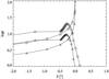Fig. 5 Comparison of line center optical path for spherical and plane-parallel geometry (triangles for MgH , and squares for C2).

4.2. Line intensities and polarization in the absence of magnetic fields

Figure 6 shows the emergent intensities at line center for the MgH and C₂ lines, for spherical geometry with FALC and FALX models, as functions of limb distance. Both lines go into emission above the solar limb, for limb distances shorter than 0.4 arcsec, and quickly disappear at greater limb distances. This is consistent with the observations reported by Faurobert & Arnaud (2002). When observed inside the limb, both lines are very weak absorption lines, which is barely seen in Fig. 6. The emission seen above the limb cannot be modeled in plane-parallel geometry.

Figure 7 presents the comparison of the emergent polarization at line centers, as functions of δ, computed in spherical and plane-parallel geometries, with FALC and FALX models. Both geometries give the same results at limb distances larger than 5′′ in absolute value, but they differ significantly at smaller limb distances. We notice that the polarization rate shows a maximum, in absolute value, for the lines of sight where the optical path shows a maximum (see Fig. 5). That can be qualitatively explained in the following way: as the slab optical thickness increases, the probability that a photon will be scattered in the line increases, so the polarization increases. At a greater distance above the limb the line optical depth decreases. This gives rise to the local polarization maximum that we see in Fig. 7. At even greater distances from the limb, when the line has disappeared, the polarization starts increasing again. We then see the continuum polarization only, and it increases because continuum scattering increases in the low chromosphere. We notice that with the FALC model, values of the polarization maxima between 2% and 2.5% are consistent with the measurements reported by Faurobert & Arnaud (2002), for the molecular lines seen in emission above the solar limb. We also want to draw attention to observations by Qu et al. (2009), where very high linear polarization (up to 10% for some C₂ lines) is found in the region where those lines are seen in emission. With FALX we recover the same general behaviour as with the FALC model, but with much higher polarization rates, the maximum reaches values around 10%. Such high rates have not been observed close to the solar limb.

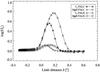Fig. 6 Intensity at line center divided by the continuum intensity, in both models as a function of limb distance. When observed above the limb, lines are seen in emission, but quickly disappear.

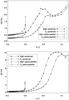Fig. 7 Linear polarization at line center as a function of limb distance for the MgH line (asterisks for spherical and triangles for plane-parallel case) and the C2 line (diamonds for spherical and squares for plane-parallel case). Upper panel: FALC model. Lower panel: FALX model.

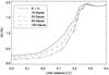Fig. 8 Limb polarization at the C2 line center versus limb distance plotted for different values of a depth-independent turbulent magnetic field.

4.3. Hanle effect of microturbulent magnetic fields

Figure 8 shows the rate of linear polarization obtained in the C₂ line for lines of sight close to the limb, in the presence of depth-independent microturbulent magnetic fields, between 0 and 100 Gauss. We observe the well known Hanle depolarization at line center. As expected, when observing above 0.4′′ from the limb, only continuum radiation remains, which is insensitive to magnetic fields. The best region, as far as the sensitivity of Hanle diagnostics is concerned, corresponds to lines of sight located within 0.3′′ from the limb. They give access to the magnetic field in the upper photosphere in the region of the temperature minimum.

5. Conclusion

In this paper we were interested in the diagnostics content of the limb polarization in the molecular lines of MgH and C₂. Accounting for the sphericity of the solar atmosphere, we investigated the limb variations of the scattering polarization in two unblended lines of MgH and C₂, which were previously observed by Faurobert & Arnaud (2002) above the solar limb. As scattering polarization is sensitive to inelastic and elastic collisions, we first used observations performed on the solar disk, as reported in Gandorfer’s Atlas (Gandorfer 2000), to estimate the relevant collision cross-sections. Inelastic collision rates for

both the MgH and C₂ lines were obtained by fitting the intensity at line centers. To to derive the elastic depolarizing collision rates in the C₂ line, we followed the same differential Hanle effect method as introduced by Bommier et al. (2006) for the MgH line. We found that inelastic collision rates are significantly higher than what was previoulsy assumed for these molecular lines, whereas elastic depolarizing collision rates for the C₂ line have the same order of magnitude as for the MgH line investigated in Bommier et al. (2006).

We have found that the line scattering polarizations show maxima of a few percent at about 0.3 arcsec above the limb, where the lines are in emission. The orders of magnitude of these polarization maxima are consistent with the observed rates when the FALC quiet Sun model is used, but the FALX model leads to much higher polarization rates.

The polarization maxima are sensitive to the Hanle effect of weak magnetic fields between 0 and 100 Gauss lying in the region of the temperature minimum between the upper photosphere and the lower chromosphere. More limb observations are needed to make use of the differential Hanle effect in different molecular lines in order to investigate this region. Such observations require few scattered light in the instrument and good seeing conditions.

Acknowledgments

Ivan Milić is grateful to the Observatoire de la Côte d’Azur for supporting this work through a Poincaré Junior fellowship and to the CNRS for a grant from the Programme National Soleil-Terre. We also acknowledge the support of the Ministry of Education and Science of the Republic of Serbia through the project 176004, “Stellar physics”.

References

All Tables

All Figures

	Fig. 1 Geometry of radiative transfer with sphericity taken into account. The line of sight with impact parameter rk is located at height h above the solar limb, i.e. rk = R⊙ + h. At depth point rd, the heliocentric angle of the line of sight is θd.
In the text

Fig. 2 C2 and MgH line profiles computed at 9′′ inside the solar limb with the FALC model, for different values of the parameter α defined in Eq. (15). Upper panel: MgH line, α values result in ϵ = 0.0025, 0.024, 0.2, 0.71 at 200 km above the base of the photosphere. Middle panel: C2 line. Corresponding values of ϵ = 0.007, 0.065, 0.41, 0.87. Lower panel: computed profiles for best-fitting values of α parameter(dashed line) compared with the observations from the atlas (full line).

In the text

	Fig. 3 C2 and MgH line polarization rates computed with the FALC model, for different values of the parameter α defined in Eq. (15). Upper two panels: MgH line; lower two panels: C2 line.
In the text

	Fig. 4 Upper panel: height variations in the lower level population of the MgH line in logarithmic scale (full line), probability of line photon collisional destruction, ϵ in units of 10-2 (asterisks), and collisional depolarization coefficient Wc (squares), computed with the FALC quiet Sun model. Bottom panel: same quantities for the C2 line.
In the text

	Fig. 5 Comparison of line center optical path for spherical and plane-parallel geometry (triangles for MgH , and squares for C2).
In the text

	Fig. 6 Intensity at line center divided by the continuum intensity, in both models as a function of limb distance. When observed above the limb, lines are seen in emission, but quickly disappear.
In the text

	Fig. 7 Linear polarization at line center as a function of limb distance for the MgH line (asterisks for spherical and triangles for plane-parallel case) and the C2 line (diamonds for spherical and squares for plane-parallel case). Upper panel: FALC model. Lower panel: FALX model.
In the text

	Fig. 8 Limb polarization at the C2 line center versus limb distance plotted for different values of a depth-independent turbulent magnetic field.
In the text

References

- Asensio Ramos, A., & Trujillo Bueno, J. 2005, ApJ, 635, L109 [NASA ADS] [CrossRef] [Google Scholar]
- Atanacković-Vukmanović, O., Crivellari, L., & Simonneau, E. 1997, ApJ, 487, 735 [NASA ADS] [CrossRef] [Google Scholar]
- Avrett, E. H. 1995, in Infrared tools for solar astrophysics: What’s next?, ed. J. R. Kuhn, & M. J. Penn, 303 [Google Scholar]
- Avrett, E. H., & Loeser, R. 1984, Line transfer in static and expanding spherical atmospheres, ed. W. Kalkofen, 341 [Google Scholar]
- Berdyugina, S. V., & Fluri, D. M. 2004, A&A, 417, 775 [NASA ADS] [CrossRef] [EDP Sciences] [Google Scholar]
- Berdyugina, S. V., Stenflo, J. O., & Gandorfer, A. 2002, A&A, 388, 1062 [NASA ADS] [CrossRef] [EDP Sciences] [Google Scholar]
- Berdyugina, S. V., Solanki, S. K., & Frutiger, C. 2003, A&A, 412, 513 [NASA ADS] [CrossRef] [EDP Sciences] [Google Scholar]
- Bommier, V., Landi Degl’Innocenti, E., Feautrier, N., & Molodij, G. 2006, A&A, 458, 625 [NASA ADS] [CrossRef] [EDP Sciences] [Google Scholar]
- Chandrasekhar, S. 1960, Radiative transfer, ed. S. Chandrasekhar [Google Scholar]
- Faurobert, M., & Arnaud, J. 2002, A&A, 382, L17 [NASA ADS] [CrossRef] [EDP Sciences] [Google Scholar]
- Faurobert, M., & Arnaud, J. 2003, A&A, 412, 555 [NASA ADS] [CrossRef] [EDP Sciences] [Google Scholar]
- Faurobert, M., Arnaud, J., Vigneau, J., & Frisch, H. 2001, A&A, 378, 627 [NASA ADS] [CrossRef] [EDP Sciences] [Google Scholar]
- Fontenla, J. M., Avrett, E. H., & Loeser, R. 1993, ApJ, 406, 319 [NASA ADS] [CrossRef] [Google Scholar]
- Gandorfer, A. 2000, The Second Solar Spectrum: A high spectral resolution polarimetric survey of scattering polarization at the solar limb in graphical representation, Vol. I: 4625 Å to 6995 Å, ed. A. Gandorfer [Google Scholar]
- Grevesse, N., Asplund, M., Sauval, A. J., & Scott, P. 2010, Ap&SS, 328, 179 [NASA ADS] [CrossRef] [Google Scholar]
- Herzberg, G. 1950, Molecular spectra and molecular structure, Vol. 1: Spectra of diatomic molecules, ed. G. Herzberg [Google Scholar]
- Landi Degl’Innocenti, E. 2006, in ASP Conf. Ser. 358, ed. R. Casini, & B. W. Lites, 293 [Google Scholar]
- Qu, Z. Q., Zhang, X. Y., Xue, Z. K., et al. 2009, ApJ, 695, L194 [NASA ADS] [CrossRef] [Google Scholar]
- Sauval, A. J., & Tatum, J. B. 1984, ApJS, 56, 193 [NASA ADS] [CrossRef] [Google Scholar]
- Shapiro, A. I., Fluri, D. M., Berdyugina, S. V., Bianda, M., & Ramelli, R. 2011, A&A, 529, A139 [NASA ADS] [CrossRef] [EDP Sciences] [Google Scholar]
- Stenflo, J. O. 2005, A&A, 429, 713 [NASA ADS] [CrossRef] [EDP Sciences] [Google Scholar]
- Stenflo, J. O., & Stenholm, L. 1976, A&A, 46, 69 [NASA ADS] [Google Scholar]