© ESO, 2012

1. Introduction

HH 158, the jet from DG Tauri, was first reported by Mundt & Fried (1983), who presented an Hα image showing a well-defined HH knot at  ~8″ to the SW of the star connected to DG Tau itself by a faint bridge. High-resolution spectroscopy of this jet was presented by Mundt et al. (1983) and Solf & Böhm (1993). In this paper, the jet emission was traced to within  ~0.′′2 from DG Tau.

DG Tau is located in the sky approximately in between the L1495 region and the star HP Tau. There are accurate distance determinations from very long baseline interferometry geometric parallax to both the L1495 region (131.5 pc; Torres et al. 2007, 2009) and HP Tau (161 pc; Torres 2009). Here we adopt for DG Tau a distance of 150 pc, intermediate to those of L1495 and HP Tau.

The proper motions of the knots observed up to distances of  ~10″ were derived by Eislöffel & Mundt (1998), using several frames obtained over a time span of about seven years, giving velocities of  ~150 km s^-1 (assuming a distance of 150 pc). Comparing adaptive optics images obtained with a two-year time base, Dougados et al. (2000) obtained proper motion velocities of  ~200 km s^-1 for the knots within  ~6″ from the source. These velocities imply a dynamical timescale of about 40 years for HH 158 at that epoch.

McGroarty & Ray (2004) suggested that two groups of HH knots (HH 702 to the SW and HH 830 to the NE) at angular distances of  ~11′ from DG Tau might be associated with the same outflow. However, McGroarty et al. (2007) showed that proper-motion measurements only support the possibility of HH 702 being associated with the outflow from DG Tau (the HH 830 knots have proper motions that are not aligned with the outflow axis). The HH 702 knots have proper motions of  ~240 km s^-1, resulting in a dynamical timescale of  ~2000 yr.

Spectroscopic data with 2D angular resolution (but with lower spectral resolution) of the region around DG Tau were presented by Lavalley et al. (1997, 2000). These observations show that some of the ejections from DG Tau have a remarkable bow shock-like morphology, and clearly show a faint counterjet to the NE (marginally seen in some of the previous observations).

Interestingly, the only optical spectrophotometric study of HH 158 with an extended wavelength coverage appears to be the one of Cohen & Fuller (1985). The spectrum described by these authors covers from  ~4000 to  ~7000 Å, and shows (reddening corrected) ratios of [O III] 5007/Hβ = 0.28, [O I] 6300/Hα = 0.30, [N II] 6548+83/Hα = 0.64 and [S II] 6716+31/Hα = 0.69. These observed [O III]/Hβ and [S II]/Hα ratios identify HH 158 as a high-excitation HH object (see Raga et al. 1996).

More recent work has focused on the low-excitation lines. The paper of Solf & Böhm (1993, mentioned above) and the more recent papers of Bacciotti et al. (2000) and Coffey et al. (2007, 2008, who present red and near-UV STIS spectra), and Pyo et al. (2003, who study the [Fe II] 1.644 μm emission) do not cover the blue region of the spectrum. Because of this, the [O III] 5007 emission reported by Cohen & Fuller (1985) has not been re-observed.

Herczeg et al. (2006) obtained far-ultraviolet (FUV) spectra of DG Tauri, reporting the detection of fluorescent H₂ lines, and the non-detection of lines like CIV 1549, which would be expected in the spectrum of a high-excitation HH object. This non-detection possibly indicates that the high-excitation emission region detected by Cohen & Fuller (1985) might be absent two decades later, or that it lies outside the region sampled by the slit in the STIS spectrum of Herczeg et al. (2006).

The high-excitation nature of HH 158 has been confirmed by the somewhat surprising detection of extended X-ray emission along the outflow (Güdel et al. 2005, 2007, 2008, 2011; Schneider & Schmitt 2008; Günther et al. 2009). These observations show an X-ray knot at  ~5″ from DG Tau, along the direction of the HH 158 flow.

We have obtained multiepoch VLA images and a red [S II] image of the region around DG Tauri to explore the current morphology of the outflow, and to be able to relate the X-ray emission to the structures observed at other wavelengths.

The base of the HH 158 flow was detected in the VLA observations of Cohen & Bieging (1982) and Bieging et al. (1984). In the present paper we present new VLA observations made at 3.6 cm in 1994, 1996, and 2009. We use these data together with the knot positions measured over the past 20 years at optical, infrared (IR) and X-ray wavelengths to derive a kinematical model for the evolution of the HH 158 outflow.

The paper is organized as follows. In Sect. 2 we describe the new and archival optical and radio continuum observations. In Sect. 3 we present the sequence of radio continuum maps and the red [S II] image. In Sect. 4 we derive a simple kinematic model for the time-evolution of the knot structure of HH 158 over the past 20 years, and a model for the free-free continuum produced in variable ejection velocity jets. Finally, the results are summarized in Sect. 5.

2. Radio and optical observations

2.1. Radio continuum observations

Because the objects in Taurus are known to exhibit relatively fast proper motions (tens of mas yr^-1, i.e. Loinard et al. 2007; Torres et al. 2007) and our observations cover long time intervals (15 years), we considered it necessary to first determine the proper motions of DG Tau to correct the positions and understand any possible changes better. For this proper-motion determination we used the three epochs observed by us and described in detail below, as well as five additional observations taken from the VLA archive. Finally, we also included an EVLA (Expanded Very Large Array) observation taken in 2011 February 26 at an average wavelength of 5.3 cm (two 1 GHz bandwidths centered at 4.56 and 7.43 GHz) in the B configuration, as part of the Gould’s Belt Distance Survey (Loinard et al. 2011). The full set of nine observations covers about 30 years. The radio positions of DG Tau as a function of time are shown in Fig. 1. The proper motions of the star derived from the fits shown in this figure are $\begin{array}{ccc}& & {\mathit{\mu }}_{\mathit{\alpha }}\cos \mathit{\delta }\mathrm{=}\mathrm{+}\mathrm{7.5}\mathrm{\pm }\mathrm{0.9} \mathrm{mas} \mathrm{yr}-1\\ & & {\mathit{\mu }}_{\mathit{\delta }}\mathrm{=}\mathrm{-}\mathrm{19.0}\mathrm{\pm }\mathrm{0.9} \mathrm{mas} \mathrm{yr}-1\mathit{.}\end{array}$These proper motions are consistent within 2-σ with those reported by Ducourant et al. (2005) from optical observations. Because our proper-motion determination is about a factor of two more accurate than that of Ducourant et al. (2005), we adopt it and use the following values for the position of DG Tau 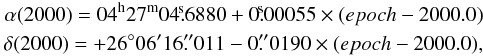$\begin{array}{ccc}\mathit{\alpha }\mathrm{\left(}\mathrm{2000}\mathrm{\right)}\mathrm{=}{\mathrm{04}}^{\mathrm{h}}{\mathrm{27}}^{\mathrm{m}}\mathrm{04}\stackrel{\mathrm{s}}{.}\mathrm{6880}\mathrm{+}\mathrm{0}\stackrel{\mathrm{s}}{.}\mathrm{00055}\mathrm{\times }\mathrm{(}\mathit{epoch}\mathrm{-}\mathrm{2000.0}\mathrm{)}& & \\ \mathit{\delta }\mathrm{\left(}\mathrm{2000}\mathrm{\right)}\mathrm{=}\mathrm{+}{\mathrm{26}}^{\mathrm{◦}}{\mathrm{06}}^{\mathrm{\prime }}\mathrm{16}\mathrm{.}\mathrm{\prime \prime }\mathrm{011}\mathrm{-}\mathrm{0}\mathrm{.}\mathrm{\prime \prime }\mathrm{0190}\mathrm{\times }\mathrm{(}\mathit{epoch}\mathrm{-}\mathrm{2000.0}\mathrm{)}\mathit{,}& & \end{array}$where epoch is the epoch given in decimal years. In the images discussed below we use this position corrected for the epoch of the observation.

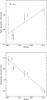Fig. 1 Position of the radio emission of DG Tau as a function of time from VLA and EVLA data. The right ascension (top) is given with respect to 04h22m and the declination (bottom) with respect to  +26° 06′. The dashed lines are least-squares fits to the data that give the proper motions discussed in the text.

The Very Large Array (VLA) observations made by us in the continuum at 3.6 cm were taken in three epochs spanning 15 years. The parameters of these observations are summarized in Table 1. The data were edited and calibrated using the software package Astronomical Image Processing System (AIPS) of the USA National Radio Astronomy Observatory (NRAO).

In Fig. 2 we show the images of the 1994 and 1996 epochs, both made in the highest angular resolution A configuration. The images are strikingly different. The 1994 image shows a single component slightly elongated in the NE-SW direction. The total flux density of this source is 0.41 ± 0.04 mJy. In contrast, the 1996 image shows two components, one is similar to that seen in 1994, but there is a new component 0.′′42 ± 0.′′01 to the SW of the first. If we assume that this new component is a knot that was ejected between the two epochs of observation and a distance of 150 pc, we derive a lower limit of 116 ± 3 km s^-1 for its velocity in the plane of the sky. The flux densities of these components are 0.44 ± 0.03 mJy (NE component, corresponding to the star) and 0.40 ± 0.03 mJy (SW component, corresponding to the knot).

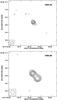Fig. 2 VLA contour images of the 3.6 cm emission associated with DG Tau for the epochs 1994.29 (top) and 1996.98 (bottom). The images were made with the weighting parameter ROBUST = 0. The contours are –3, 3, 4, 6, 8, 10, 12, 15, 20, and 25 times 19 and 15 μJy beam-1, the rms noises of the 1994.29 and 1996.98 images, respectively. The crosses mark the position of the star, determined as described in the text. The beams are shown in the bottom left corner and their dimensions are given in Table 1.

In addition to the high angular resolution observations made in 1994 and 1996, we recently made a deep integration of the region also at 3.6 cm but in the configuration C, which provides an angular resolution of  ~3″ to search for extended components around DG Tau. The image obtained from these observations is shown in Fig. 3. Two components dominate this image: a bright one with a flux density of 1.47 ± 0.02 mJy coincident with the star and a fainter one at 6.′′98 ± 0.′′40 to the SW of the star and with a flux density of 0.15 ± 0.02 mJy. We attribute this second source to a knot ejected in the past by DG Tau.

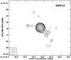Fig. 3 VLA contour images of the 3.6 cm emission associated with DG Tau for the epoch 2009.62. The image was made with the weighting parameter ROBUST = 5 to emphasize extended structure. The contours are –3, 3, 4, 6, 8, 10, 12, 15, 20, 30, 40, 60, 80, and 100 25 times 8.8 μJy beam-1, the rms noise of the image. The cross marks the position of the star, determined as described in the text. The beam is shown in the bottom left corner and its dimensions are given in Table 1.

2.2. Optical observations

In order to see the present optical structure of the HH 158 outflow, we have obtained an image of this object in the night of February 23, 2010. The narrow band image of DG Tau was obtained at the 2.6 m Nordic Optical Telescope (NOT) of the Roque de Los Muchachos Observatory (La Palma, Spain) using the Service Time mode facility. The image was obtained with the Andalucia Faint Object Spectrograph and Camera (ALFOSC) in imaging mode. The detector was an E2V 2K × 2K CCD with a pixel size of 13.5 μm, providing a plate scale of 0.19 arcsec pixel^-1. A [S II] filter (central wavelength λ = 6725 Å, FWHM = 60 Å) was used to obtain an image of DG Tau in the [S II] 6716, 6731 Å emission lines.

Two exposures of 900 s each were combined to obtain the final image. The angular resolution during the observations, as derived from the FWHM of stars in the field of view, was of 0.9–1.0 arcsec. The images were processed with the standard tasks of the IRAF reduction package.

The [S II] image is shown in Fig. 4. In this figure we also show the positions found through paraboloidal fits to the positions of the source and of the two observed knots. Because the star is saturated, we have eliminated the central region, and carried out the fit to an unsaturated ring around the center of the PSF.

Through these fits, we deduce distances of 6.′′75 and 12.′′92 from the source to the two knots along the jet. The same positions are recovered in the two exposures to within 0.′′01. However, while the first knot shows a well-defined peak, the second knot (farther away from DG Tau) shows a diffuse structure with a width of  ~3″. Because of this lack of a well-defined peak, we did not use the second knot for calculating proper motions (see Sect. 3).

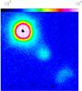Fig. 4 Red [S II] image of the HH 158 outflow. The three crosses represent the positions deduced from paraboloidal fits to DG Tau (upper left cross) and the two knots detected along HH 158. The image is displayed with a logarithmic scale (given in arbitrary units by the top bar).

3. Comparing optical, radio, and X-ray knots in DG Tau

In Table 2 we give the positions of knots along the HH 158 jet compiled by Pyo et al. (2003), together with the positions of the radio continuum knots seen in Figs. 2 and 3, the position of the knot closest to the source in our optical images (see Sect. 2.2) and the X-ray knot positions of Güdel et al. (2008, 2011).

We have carried out a least-squares fit to the knot positions x as a function of the time t of the observations of the form 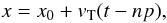$\mathit{x}\mathrm{=}{\mathit{x}}_{\mathrm{0}}\mathrm{+}{\mathit{v}}_{\mathrm{T}}\mathrm{(}\mathit{t}\mathrm{-}\mathit{np}\mathrm{)}\mathit{,}$(1)where the values of x₀, v_T and p are the same for all of the observed knots, and n is allowed to have values n = 0, 1, 2 and 3 (choosing for the individual knots the values of n that minimize the χ²). This fit assumes ballistic (i.e. constant velocity) motions. From the fit, we obtain 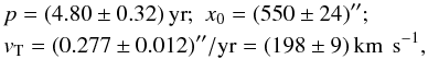$\begin{array}{ccc}& & \mathit{p}\mathrm{=}\mathrm{(}\mathrm{4.80}\mathrm{\pm }\mathrm{0.32}\mathrm{)}\hspace{0.17em}\mathrm{yr}\mathrm{;}\hspace{0.17em}\hspace{0.17em}{\mathit{x}}_{\mathrm{0}}\mathrm{=}\mathrm{(}\mathrm{550}\mathrm{\pm }\mathrm{24}{\mathrm{)}}^{\mathrm{\prime \prime }}\mathrm{;}\\ & & \end{array}$(2)where the velocity in km s^-1 was calculated assuming a distance of 150 pc to HH 158. This functional form is appropriate for a system of knots that travel with a constant velocity v_T (in ″/yr for x in arcseconds and t in years), with an ejection period p. The values of n correspond to the successive knots.

From the least-squares fit to the observed knot positions, we divide the observed knot positions into four sequences (k0, k1, k2 and k3, corresponding to n = 0, 1, 2 and 3, see Table 2). Fig. 5 shows the four resulting linear x vs. t dependencies (corresponding to n = 0, 1, 2 and 3) together with the observed knot positions.

Clearly, the observed knot positions can be interpreted as four successive knots, ejected with a period p = 4.80 yr and traveling away from the source at a velocity v_T = 198 km s^-1 (see Eq. (2) and Fig. 5). This velocity agrees well with previously measured proper motions in HH 158 (see, e.g., Dougados et al. 2000).

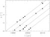Fig. 5 Positions of the knots along the HH 158 jet as a function of time. The filled circles indicate the observed optical positions, while the open circles and the stars indicate the observed radio and X-ray knot positions, respectively. The four straight lines represent the least-squares fit described in Sect. 3 (the four lines corresponding to the values n = 0, 1, 2 and 3, from left to right).

From Fig. 5 it is clear that the two radio knots reported by us are spatially correlated with optical knots that were observed close in time to the radio observations. On the other hand, the two observations of the X-ray knot (Güdel et al. 2008, 2011) show that it is the same knot that was observed as an optical knot close to the star in the early 1990’s and has moved several arc seconds since then. However, in the 2010.05 X-ray observations the knot does not show optical or radio counterparts, which should have been seen in the 2010.15 and 2009.62 observations, respectively, that we presented. This lack of counterparts adds to the puzzling nature of the X-ray knot in HH 158, whose emission requires models with shock velocities between 400 and 500 km s^-1 (Günther et al. 2009) that do not appear to be present from data at other wavelengths.

4. A model for the radio-continuum emission from a bipolar outflow

Raga et al. (1990) developed analytic and numerical models for jets from sources with intrinsically time-dependent ejection velocities. These authors showed that supersonic variabilities in the injection velocity in a supersonic flow result in the formation of two-shock structures (called working surfaces) that travel down the jet. More recently, Cantó et al. (2000) developed a method for solving the equations of a supersonic outflow with time-dependent parameters (ejection velocity and mass loss rate), based on considerations of momentum conservation for the internal working surfaces. In particular, these authors obtained solutions for a sinusoidal velocity variability with constant mass injection rate and constant injection density. In another work, González & Cantó (2002) developed a model to explain the observed free-free emission at radio frequencies around low-mass stars. In their model, the ionization is produced by internal shocks in a spherical wind that are in turn produced by periodic variations of the injection velocity. In this section, we present a model for calculating the radio-continuum (free-free) emission from a stellar flow with conical symmetry. We assume that the radiation is produced by internal working surfaces which move inside the bipolar outflow.

4.1. Dynamics of a working surface

We consider an outflow that is expelled with constant mass injection rate ṁ, and with an injection velocity v_e(τ) of the form 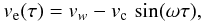$\begin{array}{ccc}{\mathit{v}}_{\mathrm{e}}\mathrm{\left(}\mathit{\tau }\mathrm{\right)}\mathrm{=}{\mathit{v}}_{\mathit{w}}\mathrm{-}{\mathit{v}}_{\mathrm{c}}\hspace{0.17em}\sin \mathrm{\left(}\mathit{\omega \tau }\mathrm{\right)}\mathit{,}& & \end{array}$(3)where v_w is the mean velocity of the flow, v_c is the amplitude of the velocity variation and ω is the angular frequency of the variation.

From the formalism developed in Cantó et al. (2000), it can be shown that the first working surface (in each cone) is formed at a distance r_c from the source given by $\begin{array}{ccc}{\mathit{r}}_{\mathrm{c}}\mathrm{=}\mathrm{-}\frac{{\mathit{v}}_{\mathit{w}}}{\mathit{\omega }} \frac{\mathrm{[}\mathrm{1}\mathrm{-}\mathrm{(}{\mathit{v}}_{\mathrm{c}}\mathit{/}{\mathit{v}}_{\mathit{w}}\mathrm{\left)} \sin \mathrm{\right(}\mathit{\omega }{\mathit{\tau }}_{\mathrm{c}}\mathrm{)}{\mathrm{]}}^{\mathrm{2}}}{\mathrm{(}{\mathit{v}}_{\mathrm{c}}\mathit{/}{\mathit{v}}_{\mathit{w}}\mathrm{)} \cos \mathit{\omega }{\mathit{\tau }}_{\mathrm{c}}}\mathit{,}& & \end{array}$(4)at a time $\begin{array}{ccc}{\mathit{t}}_{\mathrm{c}}\mathrm{=}{\mathit{\tau }}_{\mathrm{c}}\mathrm{-}\frac{\mathrm{1}}{\mathit{w}} \frac{\mathrm{[}\mathrm{1}\mathrm{-}\mathrm{(}{\mathit{v}}_{\mathrm{c}}\mathit{/}{\mathit{v}}_{\mathit{w}}\mathrm{\left)} \sin \mathrm{\right(}\mathit{\omega }{\mathit{\tau }}_{\mathrm{c}}\mathrm{\left)}\mathrm{\right]}}{\mathrm{(}{\mathit{v}}_{\mathrm{c}}\mathit{/}{\mathit{v}}_{\mathit{w}}\mathrm{)} \cos \mathrm{\left(}\mathit{\omega }{\mathit{\tau }}_{\mathrm{c}}\mathrm{\right)}}\mathit{,}& & \end{array}$(5)where τ_c is the ejection time, $\begin{array}{ccc}{\mathit{\tau }}_{\mathrm{c}}\mathrm{=}\frac{\mathit{\pi }}{\mathit{\omega }}\mathrm{-}\frac{\mathrm{1}}{\mathit{\omega }} {\sin }^{-1} [\frac{\mathrm{-}\mathrm{1}\mathrm{+}\sqrt{\mathrm{1}\mathrm{+}\mathrm{8}\mathrm{(}{\mathit{v}}_{\mathrm{c}}\mathit{/}{\mathit{v}}_{\mathit{w}}{\mathrm{)}}^{\mathrm{2}}}}{\mathrm{2}\mathrm{(}{\mathit{v}}_{\mathrm{c}}\mathit{/}{\mathit{v}}_{\mathit{w}}\mathrm{)}}]\mathrm{·}& & \end{array}$(6)Defining the variables $\overline{\mathit{\tau }}\mathrm{=}\mathrm{(}{\mathit{\tau }}_{\mathrm{1}}\mathrm{+}{\mathit{\tau }}_{\mathrm{2}}\mathrm{)}\mathit{/}\mathrm{2}$ and Δτ = (τ₂ − τ₁)/2, being τ₁ and τ₂ the ejection time of the flow directly downstream and upstream of the working surface, respectively, then the equation that describes the dynamical evolution of the working surface is $\begin{array}{ccc}{\mathit{a}}_{\mathrm{\Delta }\mathit{\tau }} {\sin }^{\mathrm{2}}\mathrm{\left(}\mathit{\omega }\mathit{\tau ̅}\mathrm{\right)}\mathrm{+}{\mathit{b}}_{\mathrm{\Delta }\mathit{\tau }} \sin \mathrm{\left(}\mathit{\omega }\mathit{\tau ̅}\mathrm{\right)}\mathrm{+}{\mathit{c}}_{\mathrm{\Delta }\mathit{\tau }}\mathrm{=}\mathrm{0}\mathit{,}& & \end{array}$(7)where $\begin{array}{ccc}& & {\mathit{a}}_{\mathrm{\Delta }\mathit{\tau }}\mathrm{=}\frac{{\mathit{v}}_{\mathrm{c}}}{{\mathit{v}}_{\mathit{w}}}\mathrm{[}\mathrm{(}\mathit{\omega }\mathrm{\Delta }\mathit{\tau }{\mathrm{)}}^{\mathrm{2}}\mathrm{-}{\sin }^{\mathrm{2}}\mathrm{(}\mathit{\omega }\mathrm{\Delta }\mathit{\tau }{\mathrm{)}}^{\mathrm{]}}\mathit{,}\\ & & {\mathit{b}}_{\mathrm{\Delta }\mathit{\tau }}\mathrm{=}\mathrm{\left(}\mathit{\omega }\mathrm{\Delta }\mathit{\tau }\mathrm{\right)}[\sin \mathrm{\left(}\mathit{\omega }\mathrm{\Delta }\mathit{\tau }\mathrm{\right)}\mathrm{-}\mathrm{\left(}\mathit{\omega }\mathrm{\Delta }\mathit{\tau }\mathrm{\right)}\hspace{0.17em}\cos \mathrm{\left(}\mathit{\omega }\mathrm{\Delta }\mathit{\tau }\mathrm{\right)}]\mathit{,}\\ & & {\mathit{c}}_{\mathrm{\Delta }\mathit{\tau }}\mathrm{=}\frac{{\mathit{v}}_{\mathrm{c}}}{{\mathit{v}}_{\mathit{w}}} \sin \mathrm{\left(}\mathit{\omega }\mathrm{\Delta }\mathit{\tau }\mathrm{\right)}\hspace{0.17em}[\sin \mathrm{\left(}\mathit{\omega }\mathrm{\Delta }\mathit{\tau }\mathrm{\right)}\mathrm{-}\mathrm{\left(}\mathit{\omega }\mathrm{\Delta }\mathit{\tau }\mathrm{\right)} \cos \mathrm{\left(}\mathit{\omega }\mathrm{\Delta }\mathit{\tau }\mathrm{\right)}\\ & & \end{array}$The  +  sign in the solution of Eq. (7) gives the solution with |sin(ωτ)| ≤ 1. Using Δτ as the free parameter (in the interval  [0,π/ω] ), we obtain by solving Eq. (7) and find τ₁ and τ₂. We then use the formalism presented in Cantó et al. (2000) to calculate the position and velocity of the working surface.

In Fig. 6 we show an example for the position and velocity of the working surface formed in a stellar jet with a sinusoidal ejection velocity variability. In our model, we have assumed a constant mass loss rate Ṁ = 5 × 10^-8 M_⊙ yr^-1, mean velocity v_w = 300 km s^-1, amplitude v_c = 200 km s^-1, and frequency w = 1.26 yr^-1 (which corresponds to an oscillation period P ≃ 5 yr). It can be observed from the figure that the working surface is not formed in the flow instantaneously, but at a time t_c = 2.67 yr and at a distance r_c = 26.81 AU from the central star. Later, the working surface begins to be accelerated asymptotically approaching the velocity v_w.

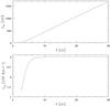Fig. 6 Position rws and velocity vws of the working surface formed in a stellar jet with a sinusoidal variation in its velocity at injection. The parameters of the model are vw = 300 km s-1, vc = 200 km s-1, and ω = 1.26 yr. We have assumed a constant mass loss rate of Ṁ = 5 × 10-8 M⊙ yr-1. The physical description of the plots is given in the text.

4.2. The geometric model

We consider a stellar outflow expelled from a central star with a sinusoidal variation in the injection velocity and constant mass loss rate. We assume conical symmetry for the jet with an opening angle of the cones θ_a, and an inclination angle between the outflow axis and the plane of the sky θ_i. Figure 7 shows a schematic diagram of the bipolar ejection.

A periodical variation in the ejection velocity (Eq. (3)) generates a set of outgoing working surfaces. Assuming that the working surfaces do not lose mass sideways, we can apply the results presented in Sect. 3.1 to obtain their dynamical properties (position and velocity as functions of time). It is possible to construct analytic (or semi-analytic) models of working surfaces in variable jets under one of the two following assumptions:

• the working surfaces eject sideways the entire material thatpasses through the two shocks (associated with the workingsurface), so that the equation of motion is determined by a rampressure balance condition,

• most of the material that goes through the shocks stays within the working surface, so that a center-of-mass formalism can be constructed.

If one compares predictions from (semi) analytic models (with these two assumptions) with axisymmetric numerical simulations, it is clear that the more realistic, axisymmetric solutions to the Euler equation lie in between the analytic models (see, e.g., Cabrit & Raga 2000). In general, the mass conservation assumption is preferred because it leads to fully analytic solutions for many forms of the ejection variability (Cantó et al. 2000), the ram pressure balance condition leads to an ordinary differential equation that normally has to be integrated numerically (see Raga & Cantó 1998). Indeed, the models computed under the two approximations described above do not have strong differences, so that the choice of one over the other does not introduce significant differences with more realistic jet models (i.e., axisymmetric numerical simulations).

Under these assumptions, the first working surface forms at a time t_c, the second one forms after one period P, and so on. In this case, the equation that describes the dynamical evolution of the working surfaces is $\begin{array}{ccc}\sin \mathrm{\left[}\mathrm{\right(}\mathrm{2}\mathit{k}\mathrm{+}\mathrm{1}\mathrm{)} \mathit{\pi }\mathrm{-}\mathit{\omega }\mathit{\tau ̅}\mathrm{]}\mathrm{=}\frac{\mathrm{-}{\mathit{b}}_{\mathrm{\Delta }\mathit{\tau }}\mathrm{+}{\mathrm{(}{\mathit{b}}_{\mathrm{\Delta }\mathit{\tau }}^{\mathrm{2}}\mathrm{-}\mathrm{4} {\mathit{a}}_{\mathrm{\Delta }\mathit{\tau }}{\mathit{c}}_{\mathrm{\Delta }\mathit{\tau }}\mathrm{)}}^{\mathrm{1}\mathit{/}\mathrm{2}}}{\mathrm{2} {\mathit{a}}_{\mathrm{\Delta }\mathit{\tau }}}\mathit{,}& & \end{array}$(11)where k is a non-negative integer (0, 1, 2,...). The solution of Eq. (11) with k = 0 gives the dynamics of the first working surface, and, in general, the solution with k = j − 1 gives the dynamical evolution of the jth working surface.

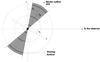Fig. 7 Schematic diagram showing a bipolar ejection with conical symmetry from a central star. The opening angle of the cones is θa and the inclination angle of the outflow axis [z′] with the plane of the sky  [y,z]  is θi. The axes y = y′ are perpendicular to the figure.

In order to obtain the flux density from the bipolar outflow, we must find the conditions that indicate whether or not a working surface is intersected by a given line of sight. In our simplified model, we assume that every working surface can be described as a portion of a sphere (a polar cap), whose physical size depends on the opening angle θ_a and its position from the central source. Thus, let  [x,y,z]  and  [x′,y′,z′]  be two frames of reference shown in Fig. 7. Every point of the jth working surface (at a distance r_ws [j]  from the central star) satisfies the equation of a sphere in both reference systems, that is, $\begin{array}{ccc}{\mathit{r}}_{\mathit{ws}\mathrm{\left[}\mathit{j}\mathrm{\right]}}^{\mathrm{2}}\mathrm{=}{\mathit{x}}^{\mathrm{\prime }\mathrm{2}}\mathrm{+}{\mathit{y}}^{\mathrm{\prime }\mathrm{2}}\mathrm{+}{\mathit{z}}^{\mathrm{\prime }\mathrm{2}}\mathrm{=}{\mathit{x}}^{\mathrm{2}}\mathrm{+}{\mathit{y}}^{\mathrm{2}}\mathrm{+}{\mathit{z}}^{\mathrm{2}}\mathit{,}& & \end{array}$(12)and, therefore, $\begin{array}{ccc}\mathit{x}\mathrm{=}\mathrm{\pm }\hspace{0.17em}{\mathrm{(}{\mathit{r}}_{\mathit{ws}\mathrm{\left[}\mathit{j}\mathrm{\right]}}^{\mathrm{2}}\mathrm{-}{\mathit{y}}^{\mathrm{2}}\mathrm{-}{\mathit{z}}^{\mathrm{2}}\mathrm{)}}^{\mathrm{1}\mathit{/}\mathrm{2}}\mathit{,}& & \end{array}$(13)where the symbol  ±  indicates the possibility that a line of sight intersects twice the working surface.

Therefore, the transformation equations between the two frames of reference are $\begin{array}{ccc}& & {\mathit{x}}^{\mathrm{\prime }}\mathrm{=}\mathrm{\pm }{\mathrm{(}{\mathit{r}}_{\mathit{ws}\mathrm{\left[}\mathit{j}\mathrm{\right]}}^{\mathrm{2}}\mathrm{-}{\mathit{y}}^{\mathrm{2}}\mathrm{-}{\mathit{z}}^{\mathrm{2}}\mathrm{)}}^{\mathrm{1}\mathit{/}\mathrm{2}} \cos {\mathit{\theta }}_{\mathit{i}}\mathrm{-}\mathit{z} \sin {\mathit{\theta }}_{\mathit{i}}\mathit{,}\\ & & {\mathit{y}}^{\mathrm{\prime }}\mathrm{=}\mathit{y,}\\ & & \end{array}$(14)The intersection conditions of the jth working surface, formed in the approaching (z′ > 0) cone or the receding (z′ < 0) cone, are obtained by comparing Eq. (14) with the edges of the caps ( ± r_ws [j]    cos   θ_a). As a consequence, the jth working surface is intersected by a given line of sight when $\begin{array}{ccc}{\mathit{z}}^{\mathrm{\prime }}\mathrm{\ge }{\mathit{r}}_{\mathit{ws}\mathrm{\left[}\mathit{j}\mathrm{\right]}} \cos {\mathit{\theta }}_{\mathit{a}}\mathit{,}& & \end{array}$(15)or $\begin{array}{ccc}{\mathit{z}}^{\mathrm{\prime }}\mathrm{\le }\mathrm{-}{\mathit{r}}_{\mathit{ws}\mathrm{\left[}\mathit{j}\mathrm{\right]}} \cos {\mathit{\theta }}_{\mathit{a}}\mathit{.}& & \end{array}$(16)Assuming that the observer is located at a distance D from the source, a given line of sight intersects the plane of the sky  [y,z]  at the point (D   sin   Θ   sin   Φ,D   sin   Θ   cos   Φ), where Θ and Φ are the inclination and the azimuthal angles, respectively. From Eqs. (14)–(16) we obtain the intersection conditions in terms of these new variables, $\begin{array}{ccc}& & \mathrm{\pm }{\mathrm{(}{\mathit{r}}_{\mathit{ws}\mathrm{\left[}\mathit{j}\mathrm{\right]}}^{\mathrm{2}}\mathrm{-}{\mathit{D}}^{\mathrm{2}} {\sin }^{\mathrm{2}}\mathrm{\Theta } {\sin }^{\mathrm{2}}\mathrm{\Phi }\mathrm{-}{\mathit{D}}^{\mathrm{2}}{\sin }^{\mathrm{2}}\mathrm{\Theta }{\cos }^{\mathrm{2}}{\mathrm{\Phi }}^{\mathrm{)}}}^{\mathrm{1}\mathit{/}\mathrm{2}} \sin {\mathit{\theta }}_{\mathit{i}}\\ & & \end{array}$(17)or $\begin{array}{ccc}& & \mathrm{\pm }{\mathrm{(}{\mathit{r}}_{\mathit{ws}\mathrm{\left[}\mathit{j}\mathrm{\right]}}^{\mathrm{2}}\mathrm{-}{\mathit{D}}^{\mathrm{2}}{\sin }^{\mathrm{2}}\mathrm{\Theta }{\sin }^{\mathrm{2}}\mathrm{\Phi }\mathrm{-}{\mathit{D}}^{\mathrm{2}}{\sin }^{\mathrm{2}}\mathrm{\Theta }{\cos }^{\mathrm{2}}{\mathrm{\Phi }}^{\mathrm{)}}}^{\mathrm{1}\mathit{/}\mathrm{2}}\sin {\mathit{\theta }}_{\mathit{i}}\\ & & \end{array}$(18)where we have assumed that the observer is far enough removed that all points of the polar caps are located at the same distance from the observer (D ≫ r_ws [j] ).

4.3. Predicted radio-continuum emission

We consider the model described in Sect. 3.2. First, we add the optical depths of the working surfaces intersected by each line of sight to obtain the total optical depth along this line of sight. Then, we use this optical depth to estimate the intensity emerging from this direction. Finally, the total flux emitted by the system can be estimated by integrating this intensity over the solid angle.

Using the numerical models developed by Ghavamian & Hartigan (1998) for the free-free emission for a planar interstellar shocks, González & Cantó (2002) estimated the average optical depth of a shock wave. Assuming an average excitation temperature of 10⁴ K, these authors found that their results can be represented by ${\mathit{\tau }}_{\mathit{\nu }}\mathrm{=}\mathit{\beta }\hspace{0.17em}{\mathit{n}}_{\mathrm{0}}\hspace{0.17em}{\mathit{\upsilon }}_{\mathrm{s}}^{\mathit{\gamma }}\hspace{0.17em}{\mathit{\nu }}^{-2.1}$, where n₀ is the preshock density, υ_s the shock velocity, and ν is the frequency. The constants β and γ depend on the shock speed. We note that the optical depth of each working surface has the the contribution of the internal and external shocks. Using this representation, the optical depth of the jth working surface is given by $\begin{array}{ccc}{\mathit{\tau }}_{\mathit{ws}\mathrm{\left[}\mathit{j}\mathrm{\right]}}\mathrm{=}[{\mathit{\beta }}_{\mathrm{e}} {\mathit{\upsilon }}_{\mathrm{es}}^{{\mathit{\gamma }}_{\mathrm{e}}}\mathrm{\left(}{\mathit{t}}_{\mathit{j}}\mathrm{\right)} {\mathit{n}}_{\mathrm{0}\mathit{,}\mathrm{1}}\mathrm{\left(}{\mathit{t}}_{\mathit{j}}\mathrm{\right)}\mathrm{+}{\mathit{\beta }}_{\mathit{i}} {\mathit{\upsilon }}_{\mathit{is}}^{{\mathit{\gamma }}_{\mathit{i}}}\mathrm{\left(}{\mathit{t}}_{\mathit{j}}\mathrm{\right)} {\mathit{n}}_{\mathrm{0}\mathit{,}\mathrm{2}}\mathrm{\left(}{\mathit{t}}_{\mathit{j}}\mathrm{\right)}] {\mathit{\nu }}^{-2.1}\mathit{,}& & \end{array}$(19)where n_0,1 is the preshock density of the external shock, and n_0,2 is the preshock density of the internal shock at its time of dynamical evolution t_j = t − (j − 1)P.

At a given line of sight (specified by the angles Θ and Φ), we add the contribution of the ith intersected working surfaces to obtain the total optical depth τ_ν(Θ,Φ) along this line of sight, that is, $\begin{array}{ccc}{\mathit{\tau }}_{\mathit{\nu }}\mathrm{\left(}\mathrm{\Theta }\mathit{,}\mathrm{\Phi }\mathrm{\right)}\mathrm{=}\sum _{\mathit{j}\mathrm{=}\mathrm{1}}^{\mathit{i}} \frac{{\mathit{\tau }}_{\mathit{ws}\mathrm{\left[}\mathit{j}\mathrm{\right]}} \mathrm{\left(}\mathrm{\Theta }\mathit{,}\mathrm{\Phi }\mathrm{\right)}}{{\mathit{\mu }}_{\mathit{j}}}\mathit{,}& & \end{array}$(20)where μ_j = cos   θ_j, being θ_j the angle between the line of sight and the normal vector to the jth working surface at the intersection point. It is easy to show that μ_j can be written as $\begin{array}{ccc}{\mathit{\mu }}_{\mathit{j}}\mathrm{=}[\mathrm{1}\mathrm{+}\frac{\stackrel{}{{{\mathit{r}}_{\mathit{ws}\mathrm{\left[}\mathrm{1}\mathrm{\right]}}^{\mathrm{2}}}_{\mathrm{˜}}}}{\stackrel{}{{{\mathit{r}}_{\mathit{ws}\mathrm{\left[}\mathit{j}\mathrm{\right]}}^{\mathrm{2}}}_{\mathrm{˜}}}} \mathrm{(}{\mathit{\mu }}_{\mathrm{1}}\mathrm{-}\mathrm{1}\mathrm{)}{]}^{\mathrm{1}\mathit{/}\mathrm{2}}\mathit{.}& & \end{array}$Finally, the flux density at radio frequencies from the bipolar outflow can be calculated by 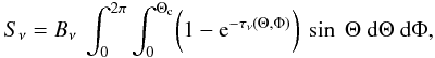$\begin{array}{ccc}{\mathit{S}}_{\mathit{\nu }}\mathrm{=}{\mathit{B}}_{\mathit{\nu }} {\mathrm{\int }}_{\mathrm{0}}^{\mathrm{2}\mathit{\pi }}{\mathrm{\int }}_{\mathrm{0}}^{{\mathrm{\Theta }}_{\mathrm{c}}}(\mathrm{1}\mathrm{-}{\mathrm{e}}^{\mathrm{-}{\mathit{\tau }}_{\mathit{\nu }}\mathrm{\left(}\mathrm{\Theta }\mathit{,}\mathrm{\Phi }\mathrm{\right)}}) \sin \mathrm{\Theta } \mathrm{d\Theta } \mathrm{d\Phi }\mathit{,}& & \end{array}$(21)where B_ν is the Planck function in the Rayleigh-Jeans approximation (B_ν = 2kT_e   ν²/c² being k the Boltzmann constant, T_e the electron temperature and c the speed of light), and Θ_c = atan   (r_ws [1] /D).

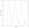Fig. 8 Predicted radio-continuum fluxes at λ = 3.6 cm for a bipolar outflow with a sinusoidal ejection velocity. The assumed parameters are vw = 300 km s-1, vc = 200 km s-1, and ω = 1.26 yr-1. We have adopted a constant mass loss rate ṁ = 5 × 10-8 M⊙ yr-1, and a distance D = 150 pc from the observer. The opening angle of the cones are θa = 30o with an inclination angle θi = 42o. The physical description of the plot is given in the text.

4.4. Numerical example

In this section we present a numerical example for the predicted radio-continuum flux at λ = 3.6 cm from a bipolar outflow with a sinusoidal ejection velocity. The opening angle of the cones is θ_a = 30^o and the inclination angle between the outflow axis and the sky plane is θ_i = 42^o. The outflow is ejected from the central star with a mean velocity v_w = 300 km s^-1, an amplitude v_c = 200 km s^-1 and with an oscillation period P = 5 yr (ω = 1.26   yr^-1). We have assumed a constant mass loss rate ṁ = 5 × 10^-8 M_⊙ yr^-1 and a distance D = 150 pc from the observer. These values are consistent with the parameters estimated from HH 158 and other jets from low-mass young stars (Eislöffel et al. 2000; Pyo et al. 2003; Agra-Amboage et al. 2011).

In Fig. 8 we present our results. Once the first working surfaces (in both cones) are formed at a time t = 2.67 yr (see, also, Fig. 6), the flux increases, reaching a maximum value of S₈.46   GHz ~ 0.5 mJy at t ≃ 4 yr. Afterward, the emission decreases until new working surfaces are formed in the outflow and the flux increases again. We note that the flux density shows a periodical behavior with the same period as that of the injection velocity variability. Finally, we note from the figure that the predicted values of the flux density agree with the radio observations of HH 158 reported in Sect. 2.

5. Summary and conclusions

We presented an analysis of archive and new Very Large Array observations of DG Tau that detect emission from knots in the jet associated with this star. Radio knots were detected in the 1996.98 and 2009.62 data and were found to correlate with optical knots in observations made close in time to the radio observations. One of these optical observations was provided by us in this paper. In contrast, the X-ray knot that was observed in the Güdel et al. (2011) data does not coincide with the radio/optical knot and appears to be part of a different, later ejection that was first detected as a moving optical knot in the early 1990’s.

All observed knot positions (optical, radio, and X-ray) can be interpreted as four successive knots, ejected with a period p = 4.80 yr and traveling away from the source at a velocity v_T = 198 km s^-1. The next knot ejection is expected to take place around epoch 2014.0.

We successfully modeled the observed radio continuum emission in terms of working surfaces produced in a jet with a velocity at injection that varies sinusoidally with time.

Acknowledgments

The National Radio Astronomy Observatory is a facility of the National Science Foundation operated under cooperative agreement by Associated Universities, Inc. The paper is partially based on observations made with the Nordic Optical Telescope, operated on the island of La Palma jointly by Denmark, Finland, Iceland, Norway, and Sweden, in the Spanish Observatorio del Roque de los Muchachos of the Instituto de Astrofísica de Canarias. L.F.R., A.G.R., J.C., L.L. and L.Z. acknowledge the financial support of DGAPA, UNAM and CONACyT, México. R.F.G. ackowledges support from grant PAPIIT IN100511-2, UNAM, México. L.L. is indebted to the Alexander von Humboldt Stiftung and the Guggenheim Memorial Foundation for financial support.

References

All Tables

All Figures

	Fig. 1 Position of the radio emission of DG Tau as a function of time from VLA and EVLA data. The right ascension (top) is given with respect to 04h22m and the declination (bottom) with respect to  +26° 06′. The dashed lines are least-squares fits to the data that give the proper motions discussed in the text.
In the text

Fig. 2 VLA contour images of the 3.6 cm emission associated with DG Tau for the epochs 1994.29 (top) and 1996.98 (bottom). The images were made with the weighting parameter ROBUST = 0. The contours are –3, 3, 4, 6, 8, 10, 12, 15, 20, and 25 times 19 and 15 μJy beam-1, the rms noises of the 1994.29 and 1996.98 images, respectively. The crosses mark the position of the star, determined as described in the text. The beams are shown in the bottom left corner and their dimensions are given in Table 1.

In the text

Fig. 3 VLA contour images of the 3.6 cm emission associated with DG Tau for the epoch 2009.62. The image was made with the weighting parameter ROBUST = 5 to emphasize extended structure. The contours are –3, 3, 4, 6, 8, 10, 12, 15, 20, 30, 40, 60, 80, and 100 25 times 8.8 μJy beam-1, the rms noise of the image. The cross marks the position of the star, determined as described in the text. The beam is shown in the bottom left corner and its dimensions are given in Table 1.

In the text

	Fig. 4 Red [S II] image of the HH 158 outflow. The three crosses represent the positions deduced from paraboloidal fits to DG Tau (upper left cross) and the two knots detected along HH 158. The image is displayed with a logarithmic scale (given in arbitrary units by the top bar).
In the text

	Fig. 5 Positions of the knots along the HH 158 jet as a function of time. The filled circles indicate the observed optical positions, while the open circles and the stars indicate the observed radio and X-ray knot positions, respectively. The four straight lines represent the least-squares fit described in Sect. 3 (the four lines corresponding to the values n = 0, 1, 2 and 3, from left to right).
In the text

	Fig. 6 Position rws and velocity vws of the working surface formed in a stellar jet with a sinusoidal variation in its velocity at injection. The parameters of the model are vw = 300 km s-1, vc = 200 km s-1, and ω = 1.26 yr. We have assumed a constant mass loss rate of Ṁ = 5 × 10-8 M⊙ yr-1. The physical description of the plots is given in the text.
In the text

	Fig. 7 Schematic diagram showing a bipolar ejection with conical symmetry from a central star. The opening angle of the cones is θa and the inclination angle of the outflow axis [z′] with the plane of the sky  [y,z]  is θi. The axes y = y′ are perpendicular to the figure.
In the text

Fig. 8 Predicted radio-continuum fluxes at λ = 3.6 cm for a bipolar outflow with a sinusoidal ejection velocity. The assumed parameters are vw = 300 km s-1, vc = 200 km s-1, and ω = 1.26 yr-1. We have adopted a constant mass loss rate ṁ = 5 × 10-8 M⊙ yr-1, and a distance D = 150 pc from the observer. The opening angle of the cones are θa = 30o with an inclination angle θi = 42o. The physical description of the plot is given in the text.

In the text

References

- Agra-Amboage, V., Dougados, C., Cabrit, S., & Reunanen, J. 2011, A&A, 532, A59 [NASA ADS] [CrossRef] [EDP Sciences] [Google Scholar]
- Bacciotti, F., Mundt, R., Ray, T. P., et al. 2000, ApJ, 537, L49 [NASA ADS] [CrossRef] [Google Scholar]
- Bieging, J. H., Cohen, M., & Schwartz, P. R. 1984, ApJ, 282, 699 [NASA ADS] [CrossRef] [Google Scholar]
- Cabrit, S., & Raga, A. C. 2000, A&A, 354, 667 [NASA ADS] [Google Scholar]
- Cantó, J., Raga, A., & D’Alessio, P. 2000, MNRAS, 313, 656 [NASA ADS] [CrossRef] [Google Scholar]
- Coffey, D., Bacciotti, F., Ray, T. P., Eislöffel, J., & Woitas, J. 2007, ApJ, 663, 350 [NASA ADS] [CrossRef] [Google Scholar]
- Coffey, D., Bacciotti, F., & Podio, L. 2008, ApJ, 689, 1112 [NASA ADS] [CrossRef] [Google Scholar]
- Cohen, M., & Fuller, G. A. 1985, ApJ, 296, 620 [NASA ADS] [CrossRef] [Google Scholar]
- Cohen, M., Bieging, J. H., & Schwartz, P. R. 1982, ApJ, 253, 707 [NASA ADS] [CrossRef] [Google Scholar]
- Ducourant, C., Teixeira, R., Périé, J. P., et al. 2005, A&A, 438, 769 [NASA ADS] [CrossRef] [EDP Sciences] [Google Scholar]
- Dougados, C., Cabrit, S., Lavalley, C., & Ménard, F. 2000, A&A, 357, L61 [NASA ADS] [Google Scholar]
- Eisloffel, J., Mundt, R., Ray, T. P., & Rodriguez, L. F. 2000, Protostars and Planets IV, 815 [Google Scholar]
- Ghavamian, P., & Hartigan, P. 1998, ApJ, 501, 687 [NASA ADS] [CrossRef] [Google Scholar]
- González, R. F., & Cantó, J. 2002, ApJ, 580, 459 [NASA ADS] [CrossRef] [Google Scholar]
- Güdel, M., Skinner, S. L., Briggs, K. R., et al. 2005, ApJ, 626, L53 [NASA ADS] [CrossRef] [Google Scholar]
- Güdel, M., Telleschi, A., Audard, M., et al. 2007, A&A, 468, 515 [NASA ADS] [CrossRef] [EDP Sciences] [Google Scholar]
- Güdel, M., Skinner, S. L., Audard, M., Briggs, K. R., & Cabrit, S. 2008, A&A, 478, 797 [NASA ADS] [CrossRef] [EDP Sciences] [Google Scholar]
- Güdel, M., Audard, M., Bacciotti., F., et al. 2011, Proceedings of the 16th Cool Stars Workshop, in press [arXiv:1101.2780] [Google Scholar]
- Günther, H. M., Matt, S. P., & Li, Z.-Y. 2009, A&A, 493, 579 [NASA ADS] [CrossRef] [EDP Sciences] [Google Scholar]
- Kepner, J., Hartigan, P., Yang, C., & Strom, S. 1993, ApJ, 415, L119 [NASA ADS] [CrossRef] [Google Scholar]
- Lavalley, C., Cabrit, S., Dougados, C., Ferruit, P., & Bacon, R. 1997, A&A, 327, 671 [NASA ADS] [Google Scholar]
- Lavalley, C., Cabrit, S., & Dougados, C. 2000, A&A, 356, L41 [NASA ADS] [Google Scholar]
- Loinard, L., Torres, R. M., Mioduszewski, A. J., et al. 2007, ApJ, 671, 546 [NASA ADS] [CrossRef] [Google Scholar]
- Loinard, L., Mioduszewski, A. J., Torres, R. M., et al. 2011, RMxAA, 40, 205 [Google Scholar]
- McGroarty, F., & Ray, T. P. 2004, A&A, 420, 975 [NASA ADS] [CrossRef] [EDP Sciences] [Google Scholar]
- McGroarty, F., Ray, T. P., & Froebrich, D. 2007, A&A, 467, 1197 [NASA ADS] [CrossRef] [EDP Sciences] [Google Scholar]
- Mundt, R., & Fried, J. W. 1983, ApJ, 274, L83 [NASA ADS] [CrossRef] [Google Scholar]
- Mundt, R., Brugel, E. W., & Bührke, T. 1987, ApJ, 319, 275 [NASA ADS] [CrossRef] [Google Scholar]
- Pyo, T.-S., Kobayashi, N., Hayashi, M., et al. 2003, ApJ, 590, 340 [NASA ADS] [CrossRef] [Google Scholar]
- Raga, A. C., & Cantó, J. 1998, RMxAA, 34, 73 [NASA ADS] [Google Scholar]
- Raga, A. C., Böhm, K. H., & Cantó, J. 1986, RMxAA, 32, 161 [Google Scholar]
- Raga, A. C., Cantó, J., Binette, L., & Calvet, N. 1990, ApJ, 364, 601 [NASA ADS] [CrossRef] [Google Scholar]
- Schneider, P. C., & Schmitt, J. H. M. M. 2008, A&A, 488, L13 [NASA ADS] [CrossRef] [EDP Sciences] [Google Scholar]
- Solf, J., & Böhm, K. H. 1993, ApJ, 410, L31 [NASA ADS] [CrossRef] [Google Scholar]
- Takami, M., Chrysostomoy, A., Bailey, J., et al. 2002, ApJ, 568, L53 [NASA ADS] [CrossRef] [Google Scholar]
- Torres, R. M., Loinard, L., Mioduszewski, A. J., & Rodríguez, L. F. 2007, ApJ, 671, 1813 [NASA ADS] [CrossRef] [Google Scholar]
- Torres, R. M., Loinard, L., Mioduszewski, A. J., & Rodríguez, L. F. 2009, ApJ, 698, 242 [NASA ADS] [CrossRef] [Google Scholar]