| Issue |
A&A
Volume 537, January 2012
|
|
|---|---|---|
| Article Number | A136 | |
| Number of page(s) | 6 | |
| Section | Planets and planetary systems | |
| DOI | https://doi.org/10.1051/0004-6361/201117706 | |
| Published online | 23 January 2012 | |
Research Note
Transiting exoplanets from the CoRoT space mission
XXI. CoRoT-19b: a low density planet orbiting an old inactive F9V-star⋆
1 Thüringer Landessternwarte Tautenburg, 07778 Tautenburg, Germany
e-mail: This email address is being protected from spambots. You need JavaScript enabled to view it.
2 Institut d’Astrophysique de Paris, UPMC-CNRS, UMR 7095, Institut d’Astrophysique de Paris, 75014 Paris, France
3 Laboratoire d’Astrophysique de Marseille, 38 rue Frédéric Joliot-Curie, 13388 Marseille Cedex 13, France
4 School of Physics and Astronomy, Raymond and Beverly Sackler Faculty of Exact Sciences, Tel Aviv University, Tel Aviv, Israel
5 Observatoire de Haute-Provence, Université Aix-Marseille & CNRS, 04870 St. Michel l’Observatoire, France
6 Observatoire de la Côte d’ Azur, Laboratoire Cassiopée, BP 4229, 06304 Nice Cedex 4, France
7 Department of Physics, Denys Wilkinson Building Keble Road, Oxford, OX1 3RH, UK
8 Observatoire de l’Université de Genève, 51 chemin des Maillettes, 1290 Sauverny, Switzerland
9 LESIA, UMR 8109 CNRS, Observatoire de Paris, UVSQ, Université Paris-Diderot, 5 place J. Janssen, 92195 Meudon, France
10 Institut d’Astrophysique Spatiale, Université Paris-Sud 11, 91405 Orsay, France
11 Institute of Planetary Research, German Aerospace Centre, Rutherfordstraße 2, 12489 Berlin, Germany
12 Centre for Astronomy and Astrophysics, TU Berlin, Hardenbergstraße 36, 10623 Berlin, Germany
13 LUTH, Observatoire de Paris, CNRS, Université Paris Diderot ; 5 place Jules Janssen, 92195 Meudon, France
14 Rheinisches Institut für Umweltforschung an der Universiät zu Köln, Aachener Straße 209, 50931 Köln, Germany
15 Research and Scientific Support Department, ESTEC/ESA, PO Box 299, 2200 AG Noordwijk, The Netherlands
16 Instituto de Astrofísica de Canarias, 38205 La Laguna, Tenerife, Spain
17 University of Vienna, Institute of Astronomy, Türkenschanzstraße 17, 1180 Vienna, Austria
18 Instituto de Astronomia, Geofísica e Ciências Atmosféricas, Universidade de São Paulo, Rua do Matão 1226, 05508-900 São Paulo, Brazil
19 University of Liège, Allée du 6 août 17, S. Tilman, Liège 1, Belgium
20 Space Research Institute, Austrian Academy of Science, Schmiedlstr. 6, 8042 Graz, Austria
21 Dpto. de Astrofísica, Universidad de La Laguna, 38206 La Laguna, Tenerife, Spain
22 Georg-August-Universität, Institut für Astrophysik, Friedrich-Hund-Platz 1, 37077 Göttingen, Germany
23 Department of Physics and Astronomy, Aarhus University, 8000 Aarhus C, Denmark
Received: 14 July 2011
Accepted: 24 November 2011
Abstract
Context. Observations of transiting extrasolar planets are of key importance to our understanding of planets because their mass, radius, and mass density can be determined. These measurements indicate that planets of similar mass can have very different radii. For low-density planets, it is generally assumed that they are inflated owing to their proximity to the host-star. To determine the causes of this inflation, it is necessary to obtain a statistically significant sample of planets with precisely measured masses and radii.
Aims. The CoRoT space mission allows us to achieve a very high photometric accuracy. By combining CoRoT data with high-precision radial velocity measurements, we derive precise planetary radii and masses. We report the discovery of CoRoT-19b, a gas-giant planet transiting an old, inactive F9V-type star with a period of four days.
Methods. After excluding alternative physical configurations mimicking a planetary transit signal, we determine the radius and mass of the planet by combining CoRoT photometry with high-resolution spectroscopy obtained with the echelle spectrographs SOPHIE, HARPS, FIES, and SANDIFORD. To improve the precision of its ephemeris and the epoch, we observed additional transits with the TRAPPIST and Euler telescopes. Using HARPS spectra obtained during the transit, we then determine the projected angle between the spin of the star and the orbit of the planet.
Results. We find that the host star of CoRoT-19b is an inactive F9V-type star close to the end of its main-sequence life. The host star has a mass M∗ = 1.21 ± 0.05 M⊙ and radius R∗ = 1.65 ± 0.04 R⊙. The planet has a mass of MP = 1.11 ± 0.06 MJup and radius of RP = 1.29 ± 0.03 RJup. The resulting bulk density is only ρ = 0.71 ± 0.06 g cm-3, which is much lower than that for Jupiter.
Conclusions. The exoplanet CoRoT-19b is an example of a giant planet of almost the same mass as Jupiter but a ≈30% larger radius.
Key words: planetary systems / techniques: photometric / techniques: radial velocities / techniques: spectroscopic
The CoRoT space mission, launched on December 27, 2006, has been developed and is operated by the CNES, with the contribution of Austria, Belgium, Brazil, ESA (RSSD and Science Program), Germany and Spain. Partly based on observations obtained at the European Southern Observatory at Paranal, Chile in program 184.C-0639, and partly based on observations conducted at McDonald Observatory.
© ESO, 2012
1. Introduction
The discovery of gas-giant planets orbiting their star at distances ≤ 0.1 AU more than 15 years ago was surprising, and their study is still an active field of research. A key observation for understanding these objects are those of transiting planets because they allow us to determine their true mass, radius, and full orbital parameters. For some transiting planets, it is even possible to determine the projected angle between the stellar rotation and orbital spin axes. Thus, transiting planets allow us to obtain very detailed information that is essential to constrain models of the formation and evolution of extrasolar planets.
The determination of the mass and radius and hence the density of extrasolar planets led to a rather unexpected result that planets of the same mass can have very different radii and thus very different bulk densities. Planets of very low density are possibly inflated owing to their close proximity to the host star. To aid our understanding of why close-in planets are inflated, it is essential to obtain precise values for the masses and radii of many extrasolar planets orbiting stars of different mass, temperature, luminosity, and orbital distances. Since accurate planetary parameters are crucial for modeling the structure of the planet, it is preferable to have precise measurements of a small sample of transiting exoplanets, rather than low precision measurements of a larger sample. Space-based transit search programs are ideal for this purpose because their high sensitivity and excellent time-coverage enables us to explore a wider range of planet densities, and orbital periods.
Here we present the discovery of CoRoT-19b, a planet with the mass of Jupiter but a radius that is substantially larger. By determining the properties of the planet and its host star precisely, we thus add in an important piece to the puzzle of exoplanets.
2. The CoRoT light-curves
CoRoT-19 was continuously observed with the CoRoT satellite from March 5 to 29, 2010 in the chromatic mode. The coordinates, proper motion, and brightness of the star are given in Table 1. Figure 1 shows an DSS image of the field with the mask image superimposed.
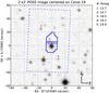 |
Fig. 1 DSS image of the field. The jagged outline at the centre is the photometric aperture mask (North is up, east is right). |
The sampling of the light-curve was 32 s, thus 65123 photometric measurements in three colours were obtained. Six full transit-like events were visible, and a seventh one was partly covered. The transit-like events are periodic with a period of 3.8971272 ± 0.000020 days. The depth of successive transits was constant to within 0.79 ± 0.02%. Figure 2 shows the monochromatic light-curve of the transit produced by the standard CoRoT pipeline (version 2.1), after combining the signal from the three-colour channels (Auvergne et al. 2009) and co-adding all transits.
CoRoT-19, coordinates, and brightness magnitudes.
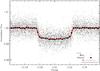 |
Fig. 2 Light-curve of CoRoT-19 obtained by CoRoT in white-light together with the best-fit model. |
The fitting of the transit lightcurve was carried out by two groups independently and both obtained consistent results (Table 5). For the light-curve modeling, we used a contamination factor of ≤0.32% and a circular orbit (see Sects. 3 and 4.2).
The first analysis used the Markov chain Monte Carlo (MCMC) algorithm described by Tegmark et al. (2004) and Holman et al. (2006) for the implementation described in Gibson et al. (2010). Using this method, we found that a/R∗ = 6.79 ± 0.20, 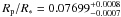 , and
, and  .
.
Transit times.
Independently of the MCMC method, we carried out another analysis using a genetic algorithm optimization. This allowed us to verify the uniqueness of the solution. The data was fitted using the model of Mandel & Agol (2002) after it had been phase-folded. The free parameters are: the epoch, the ratio of the semi-major axis (a) to the star’s radius (R∗), the ratio of the radius of the planet to stellar radius k = Rp/R∗, and the impact parameter (b = acosi/R∗, with the inclination i). We used the limb darkening coefficients published by Sing (2010) as defined by Brown et al. (2001) using the Teff, log g-values, and metallicity of the star derived in Sect. 4.3 and given in Table 5. The accuracy is thus limited only by the accuracy with which the stellar parameters were determined. The phase-folded light-curve of the transit together with the best-fit solution obtained is shown in Fig. 2. The results and the 1σ uncertainties are a/R∗ = 6.68 ± 0.13, Rp/R∗ = 0.0786 ± 0.0004, and (M∗/M⊙)1/3(R∗/R⊙)-1 = 0.64 ± 0.02. The agreement between the two methods is thus good.
The times of the mid-points of the transits are given in Table 2. The errors in the measurements are on average 2.3 min, and the difference between the calculated times of the transit are on average 2.9 min. There is no evidence of transit timing variations.
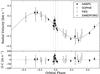 |
Fig. 3 RV-values together with the orbital fit (instrumental offset removed). |
3. Excluding a background binary within the photometric mask
Since the photometric mask of CoRoT has a size of 30″ × 16″, we must confirm that the transits are caused by CoRoT-19 and not by an eclipsing binary within the photometric mask. To demonstrate this, we took images during transit (“on”) and images out of transit (“off”) (Deeg et al. 2009). If the transit were caused by an eclipsing binary within the photometric mask, an eclipsing binary in the background would be correspondingly fainter in the image taken during transit than in the image taken out of transit. For this purpose, we used MONET (located at McDonald Observatory, USA), the OGS a 1 m telescope (located at Izaña Tenerife, Spain), the 1 m telescope of the Florence George Wise Observatory (Israel), and the Euler telescope (located at La Silla Chile). We detected only two stars within the mask, CoRoT-19, and a star that is labeled No. 5 in Fig. 1. This star has mR = 19.93 ± 0.070 mag, and leads to a contamination factor of ≤ 0.32%. Star No.5 is thus to faint to cause a transit with a depth of 0.79 ± 0.02%.
Radial velocity measurements.
After confirming that CoRoT-19 was the object experiencing a transit, we observed two additional transits with the TRAPPIST (Gillon et al. 2011), and Euler telescopes to improve the accuracy of the ephemeris. This step was important because CoRoT-19b was observed by CoRoT for only 24 days. The detection of the transit on the target with ground-based telescopes confirms again that CoRoT-19 has a transiting planet orbiting with the period and phase measured by CoRoT. The transit-times are given in Table 2.
4. Spectroscopic observations
We obtained high-resolution echelle spectra of CoRoT-19 to determine its mass, radius, and other host star properties, which were than used to derive the mass, radius and the equilibrium temperature of the planet, Teq, of the planet. The detection of the radial-velocity (RV) signal of the planet confirms the nature of the photometric transit. All RVs obtained are listed in Table 3. Figure 3 shows the phase-folded RV-measurements together with the orbit.
4.1. Radial-velocity measurements
4.1.1. HARPS
We took 19 spectra of CoRoT-19 with the HARPS spectrograph between 2010 December 15 and 2011 March 6 (Pepe et al. 2002; Mayor et al. 2003) (ESO program 184.C-0639). The spectra obtained have a resolving power λ/Δλ ≈ 115 000 and cover the region from 3780 Å to 6910 Å in 72 spectral orders. Eleven of the nineteen HARPS spectra were taken during a transit in order to detect the Rossiter-McLaughlin effect (Sect. 5), and the other spectra were used to determine the mass of the planet. The spectra were reduced and extracted using the HARPS pipeline (bias subtraction, flat-fielded, scattered light subtraction, and wavelength calibration). The sky-fibre was used to remove stray-light from the moon if necessary. The RVs were determined by using a cross-correlation method with a numerical mask that corresponds to a G2 star (Baranne et al. 1996; Pepe et al. 2002). The RV-measurements were obtained by fitting a Gaussian function to the the average cross-correlation function (CCF), after discarding the ten bluest and the two reddest orders of the spectra that were of a low signal-to-noise ratio (S/N).
4.1.2. SOPHIE
We obtained seven spectra with the SOPHIE spectrograph on the 1.93 m telescope at the Observatoire de Haute-Provence, France (Bouchy et al. 2009; Perruchot 2008). For our observation, we used the high efficiency mode, which has a resolution of λ/Δλ = 40 000 and covers the wavelength region from 3872 Å to 6943 Å in 39 spectral orders (eight bluest and five reddest orders were discarded because of the low S/N). The reduction was performed in a similar way to that for HARPS spectra.
4.1.3. FIES
Five spectra were also taken with the fibre-fed echelle spectrograph FIES, which is mounted on the 2.6 m Nordic Optical Telescope (NOT) at Roque de los Muchachos Observatory (La Palma, Spain) in program P42-216. We used the 1.3′′ high-resolution fibre, which gives a resolving power of λ/Δλ ≈ 67 000 and covers the wavelength range 3600–7400 Å. The data were reduced using standard IRAF routines. The RVs were obtained using the RV standard star HD 50692 (Udry et al. 1999), which was observed with the same instrumental set-up.
4.1.4. SANDIFORD
Two additional RV measurements were performed on spectra acquired with the Sandiford Cassegrain echelle spectrometer (SANDIFORD) mounted at the Cassegrain focus of the 2.1 m (82 inch) Otto Struve Telescope at McDonald Observatory, Texas, USA. The spectra cover the wavelength range 5000–6000 Å with a resolving power of λ/Δλ ≈ 47 000. The adopted observing strategy, data reduction, and RV-determination were the same as FIES.
4.2. The mass of the planet and its orbit
In total, we obtained 33 spectra of CoRoT-19 of which 12 were taken during transit. For the orbit determination, we excluded from the analysis all measurements taken during the transit, and the first SOPHIE measurement (BJD = 2 455 513.6) because it was a clear outlier.
Since the observations of the transits allow us to determine the period and epoch to a very high accuracy, we used these values. The best-fitting orbit was derived by minimizing the χ2 using the Downhill Simplex Algorithm (Nelder & Mead 1965). The errors given in Table 5 correspond to the 68% confidence level using the bootstrap method. The best-fit model curve is shown in Fig. 3 and the parameters obtained are given in Table 5.
The scatter around the best-fit model orbit is comparable to the typical error bar for each dataset. The errors were determined from the photon noise and the wavelength calibration (Bouchy et al. 2001). The scatter around the best-fit solution is 12.2 m s-1, 23.4 m s-1, and 8.6 m s-1 for HARPS, SOPHIE, and FIES, respectively. The two SANDIFORD measurements differ on average by 5.5 m s-1 from the fitted curve (Table 3), with a confidence level of 95% (resp. 99%) that the orbital eccentricity is smaller than 0.12 (0.15).
The detection of the RV-variations with the correct period and phase lends strong support to the planet hypothesis. However, to prove that the RV-variations are caused by the planet, we also analyzed the spectral line asymmetry, which we measured by determining the bisector of the CCF function of the HARPS spectra taken out-of-transit (Queloz et al. 2009). The lack of correlation between the bisector and the RV-variations shows that the RV-variations are caused by the planet (Fig. 4).
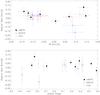 |
Fig. 4 Bisector span of the CCF versus the RV measurements (top panel) and the orbital phase (bottom panel). |
Abundances of some chemical elements for the fitted lines in the HARPS co-added spectrum. The abundances refer to the solar value and the last column reports the number of lines used.
Parameters of the planet and the star.
4.3. The properties of the host star
To determine the photospheric parameters of CoRoT-19, we constructed a master spectrum by co-adding the HARPS spectra after shifting them to the same RV zero point. The master spectrum has a S/N of 130 at 5500 Å.
Following the method described in Deleuil et al. (2008) and Bruntt et al. (2010), the spectral analysis was performed using the semi-automatic package VWA (Bruntt et al. 2002, 2008, 2010). The parameters of the star are Teff = 6090 ± 70 K, log g = 4.0 ± 0.1 [cgs], and [Fe/H] = −0.02 ± 0.10 [dex]. Using the Spectroscopy Made Easy (SME) method (Valenti & Piskunov 1996), we obtained Teff = 6200 ± 70 K, log g = 4.2 ± 0.1 [cgs], and [M/H] = 0.1 ± 0.1 [dex], which is in agreement with the VWA method. The abundances derived are given in Table 4, and all other parameters of the star are given in Table 5).
Instead of using log g from the spectroscopic analysis to determine the mass and radius of the star, we used the value M1/3R-1 obtained from the light-curve analysis, and the spectroscopically derived Teff, and [Fe/H] because the log (g) determined in this way has a smaller error than the spectroscopic determination. Since the mass and radius of the star are derived from the evolutionary tracks, the parameters of the planets also depend on the accuracy of the tracks. We thus determined these parameters using two different sets of tracks. The STAREVOL evolution tracks (Palacios, priv. comm.) yield a mass of M∗ = 1.20 ± 0.06 M⊙, and a radius of R∗ = 1.62 ± 0.08 R⊙ for the star
We also used a Bayesian estimation of stellar parameters (da Silva et al. 2006) and the evolutionary tracks published by Girardi et al. (2000) to determine the stellar parameters. These tracks were tested by Baines et al. (2009) by comparing the diameters of stars derived from the tracks with the diameters measured directly with the CHARA interferometer. Using these tracks, we obtained M∗ = 1.21 ± 0.05 M⊙, and R∗ = 1.65 ± 0.04 R⊙, which are values entirely consistent with those from STAREVOL.
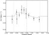 |
Fig. 5 RV-measurements taken during transit with the orbit subtracted (Rossiter-McLaughlin effect). |
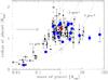 |
Fig. 6 Mass-radius diagram of the planets and brown dwarfs. CoRoT-19b is marked with a thick red point and by the arrows, all other objects discovered by CoRoT are indicated by the tick blue points, and planets discovered in other surveys are shown as small (black) points. |
By combining the radius of the star with the relative size of the planet determined from the transit curve (Table 5), we derived a radius for the planet of Rp = 1.29 ± 0.03 RJup. The absolute magnitude of the star is Mv = 3.40 ± 0.05, and the distance 770 ± 160 pc, if we take the extinction of Av = 1.2 ± 0.5 into account. The star is close to the end of the H-burning phase and has an age from four to six Gyrs. Using the HARPS spectrum, we obtained v sin i = 6 ± 1 km s-1. This means that the rotation period of the star is Prot ≥ 14 d. The star was not detected in the ROSAT all-sky survey and we did not detect either the Li i line at 6707.8 Å or an emission component in the Ca ii H &K lines in the master spectrum. In summary, the host star is an old, inactive F9 V star close to the end of its life on the main-sequence.
5. The Rossiter McLaughlin effect
The spectroscopic transit CoRoT-19 was observed with HARPS to detect the Rossiter-McLaughlin (RM) anomaly. This apparent distortion of the stellar lines profile owing to the transit of a planet in front of a rotating star allows us to measure the sky-projected angle between the planetary orbital axis and the stellar rotation axis λ (e.g. Bouchy et al. 2008). Figure 5 shows the RV-measurements obtained with HARPS after subtracting the orbit. The uncertainties were determined from the obtained χ2 surface, taking into account the errors in the K-amplitude, Vr, and i. The RM effect is marginally detected (at 2.3σ) with  deg. There is thus a hint that the system is misaligned but to only at the 2σ-level.
6. Discussion and conclusions
In Fig. 6 we present the mass-radius diagram for transiting planets and brown dwarfs. The objects marked with a large blue point are those discovered by CoRoT, the objects with small points are those detected with other instruments. The planet CoRoT-19b is indicted by a large red dot and the two arrows. The two CoRoT-planets above CoRoT-19b are CoRoT-1b (Barge et al. 2008) and CoRoT-12b Gillon et al. (2010). Their densities are 0.38 ± 0.05 and 0.31 ± 0.08 g cm-1, respectively, a bit lower than CoRoT-19b, which has 0.71 ± 0.06 g cm-1. Thus, CoRoT-19b is an example of an inflated extrasolar planet but is less extreme than the others.
Acknowledgments
The French teams are grateful to CNES for its constant support and funding of A.B., J.M.A., and C.C. The German team thanks the DLR and the BMBF for the support under grants 50 OW 0204, and 50 OW 0603. The team at the IAC acknowledges support by grants ESP2007-65480-C02-02 and AYA2010-20982-C02-02 of the Spanish Ministerio de Ciencia e Innovación. TRAPPIST is funded by the Belgian Fund for Scientific Research (Fond National de la Recherche Scientifique, FNRS) under the grant FRFC 2.5.594.09.F, with the participation of the Swiss National Science Foundation (SNF). M. Gillon and E. Jehin are FNRS Research Associates. MONET (MOnitoring NEtwork of Telescopes) is funded by the “Astronomie & Internet” program of the Alfred Krupp von Bohlen und Halbach Foundation, Essen, and operated by the Georg-August-Universität Göttingen, the McDonald Observatory of the University of Texas at Austin, and the South African Astronomical Observatory. The results are also partly based on observations performed with the FIES spectrograph at the Nordic Optical Telescope (NOT), under observing program P42-261. NOT is operated on the island of La Palma jointly by Denmark, Finland, Iceland, Norway, and Sweden, in the Spanish Observatorio del Roque de los Muchachos of the Instituto de Astrofisica de Canarias. Additional data was obtained with the Sandiford spectrograph at the 2.1 m Otto Struve telescope at McDonald Observatory (Texas, USA), and the SOPHIE spectrograph at the Observatoire de Haute-Provence, France, under observing program PNP.08A.MOUT.
References
- Auvergne, M., Bodin, P., Boisnard, L., et al. 2009, A&A, 506, 411 [NASA ADS] [CrossRef] [EDP Sciences] [Google Scholar]
- Baines, E. K., Döllinger, M. P., Cusano, F., et al. 2010, ApJ, 710, 1365 [NASA ADS] [CrossRef] [Google Scholar]
- Baranne, A., Queloz, D., Mayor, M., et al. 1996, A&AS, 119, 373 [NASA ADS] [CrossRef] [EDP Sciences] [Google Scholar]
- Barge, P., Baglin, A., Auvergne, M., et al. 2008, A&A, 482, L17 [NASA ADS] [CrossRef] [EDP Sciences] [Google Scholar]
- Bouchy, F., Pepe, F., Queloz, D. 2001, A&A, 374, 733 [NASA ADS] [CrossRef] [EDP Sciences] [Google Scholar]
- Bouchy, F., Queloz, D., Deleuil, M., et al. 2008, A&A, 482, L25 [NASA ADS] [CrossRef] [EDP Sciences] [Google Scholar]
- Bouchy, F., Hébrard, G., Udry, S., et al. 2009, A&A, 505, 853 [NASA ADS] [CrossRef] [EDP Sciences] [Google Scholar]
- Brown, T. M., Charbonneau, D., Gilliland, R. L., et al. 2001, ApJ552, 699 [Google Scholar]
- Bruntt, H., Catala, C., Garrido, R., et al. 2002, A&A, 389, 345 [NASA ADS] [CrossRef] [EDP Sciences] [Google Scholar]
- Bruntt, H., De Cat, P., & Aerts, C. 2008, A&A, 478, 487 [NASA ADS] [CrossRef] [EDP Sciences] [Google Scholar]
- Bruntt, H., Deleuil, M., Fridlund, M., et al. 2010, A&A, 519, A51 [NASA ADS] [CrossRef] [EDP Sciences] [Google Scholar]
- da Silva, L., Girardi, L., Pasquini, L., et al., A&A, 458, 609 [Google Scholar]
- Deeg, H. J., Gillon, M., Shporer, A., et al. 2009, A&A, 506, 343 [NASA ADS] [CrossRef] [EDP Sciences] [Google Scholar]
- Deleuil, M., Deeg, H. J., Alonso, R., et al. 2008, A&A, 491, 889 [NASA ADS] [CrossRef] [EDP Sciences] [Google Scholar]
- Gibson, N. P., Pollacco, D. L., Barros, S., et al. 2010, MNRAS, 401, 1917 [NASA ADS] [CrossRef] [Google Scholar]
- Gillon, M., Hatzes, A., Csizmadia, Sz., et al. 2010, A&A, 520, A97 [NASA ADS] [CrossRef] [EDP Sciences] [Google Scholar]
- Gillon, M., Jehin, E., Magain, P., et al. 2011, in Detection and Dynamics of Transiting Exoplanets, Proceedings of OHP Colloquium, 23–27 August 2010, ed. F. Bouchy, R. F. Diaz, & C. Moutou (Platypus Press) [arXiv:1101.5807] [Google Scholar]
- Girardi, L., Bressan, A., Bertelli, G., & Chiosi, C. 2000, A&AS, 141, 371 [NASA ADS] [CrossRef] [EDP Sciences] [Google Scholar]
- Holman, M. J., Winn, J. N., Latham, D. W., et al. 2006, ApJ, 652, 1715 [NASA ADS] [CrossRef] [Google Scholar]
- Mandel, K., & Agol, E. 2002, ApJ, 580, L171 [NASA ADS] [CrossRef] [Google Scholar]
- Mayor, M., Pepe, F., Queloz, D., et al. 2003, The Messenger, 114, 20 [NASA ADS] [Google Scholar]
- Nelder, J., & Mead, R. 1965, Comput. J., 7, 308 [Google Scholar]
- Pepe, F., Mayor, M., Galland, F., et al. 2002, A&A, 388, 632 [NASA ADS] [CrossRef] [EDP Sciences] [Google Scholar]
- Perruchot, S., Kohler, D., Bouchy, F., et al. 2008, in SPIE Conf. Ser., 7014 [Google Scholar]
- Queloz, D., Eggenberger, A., Mayor, M., et al. 2000, A&A, 359, L13 [NASA ADS] [Google Scholar]
- Sing, D. K. 2010, A&A, 510, 21 [Google Scholar]
- Tegmark, M., Strauss, M. A., Blanton, M. R., et al. 2004, Phys. Rev. D, 69, 103501 [CrossRef] [Google Scholar]
- Udry, S., Mayor, M., & Queloz, D. 1999, IAU Colloq. 170: Precise Stellar Radial Velocities, 185, 367 [NASA ADS] [Google Scholar]
- Valenti, J. A., & Piskunov, N. 1996, A&AS, 118, 595 [NASA ADS] [CrossRef] [EDP Sciences] [Google Scholar]
All Tables
Abundances of some chemical elements for the fitted lines in the HARPS co-added spectrum. The abundances refer to the solar value and the last column reports the number of lines used.
All Figures
|
Fig. 1 DSS image of the field. The jagged outline at the centre is the photometric aperture mask (North is up, east is right). |
| In the text | |
|
Fig. 2 Light-curve of CoRoT-19 obtained by CoRoT in white-light together with the best-fit model. |
| In the text | |
|
Fig. 3 RV-values together with the orbital fit (instrumental offset removed). |
| In the text | |
|
Fig. 4 Bisector span of the CCF versus the RV measurements (top panel) and the orbital phase (bottom panel). |
| In the text | |
|
Fig. 5 RV-measurements taken during transit with the orbit subtracted (Rossiter-McLaughlin effect). |
| In the text | |
|
Fig. 6 Mass-radius diagram of the planets and brown dwarfs. CoRoT-19b is marked with a thick red point and by the arrows, all other objects discovered by CoRoT are indicated by the tick blue points, and planets discovered in other surveys are shown as small (black) points. |
| In the text | |
Current usage metrics show cumulative count of Article Views (full-text article views including HTML views, PDF and ePub downloads, according to the available data) and Abstracts Views on Vision4Press platform.
Data correspond to usage on the plateform after 2015. The current usage metrics is available 48-96 hours after online publication and is updated daily on week days.
Initial download of the metrics may take a while.