| Issue |
A&A
Volume 536, December 2011
|
|
|---|---|---|
| Article Number | L2 | |
| Number of page(s) | 4 | |
| Section | Letters | |
| DOI | https://doi.org/10.1051/0004-6361/201118304 | |
| Published online | 02 December 2011 | |
Letter to the Editor
First results of Herschel-SPIRE observations of Titan⋆
1
LESIA–Observatoire de Paris, CNRS, Université Paris 6, Université Paris-Diderot, 5 place Jules Janssen, 92195 Meudon, France
e-mail: This email address is being protected from spambots. You need JavaScript enabled to view it.
2
University College London, Department of Physics and Astronomy, Gower Street, London WC1E 6BT, UK
3
University of Lethbridge, Institute for Space Imaging Science, Department of Physics and Astronomy, Lethbridge, Alberta T1K 3M4, Canada
4
Max-Planck-Institut für Sonnensystemforschung, Max-Planck-Str. 2, 37191 Katlenburg-Lindau, Germany
Received: 20 October 2011
Accepted: 10 November 2011
Abstract
We investigate the composition of Titan’s stratosphere from high-resolution submillimetric observations performed with the SPIRE instrument on the Herschel satellite. From the flux density spectrum measured in the 20 − 52 cm-1 interval at an apodized resolution of 0.08 cm-1, we determine the stratospheric abundances of CH4, CO, HCN, as well as the isotopic ratios 12C/13C = 87 ± 6 in CO and 96 ± 13 in HCN, 14N/15N = 76 ± 6, and 16O/18O = 380 ± 60. The last of these results is the first documented measurement of Titan’s 16O/18O ratio in CO, with a value 24% lower than the terrestrial ratio.
Key words: techniques: spectroscopic / submillimeter: planetary systems / planets and satellites: individual: Titan
Herschel is an ESA space observatory with science instruments provided by European-led Principal Investigator consortia and with important participation from NASA.
© ESO, 2011
1. Introduction
The radiation emitted by Titan in the submillimeter range is a combination of a continuum emission originating from an extended region centered at the tropopause, which includes a minor contribution from the surface (Courtin 1982), and of stratospheric emission lines superimposed on this continuum. Depending on their resolution, spectrally resolved measurements in this spectral domain allow the investigation of a variety of processes in Titan’s atmosphere, including the tropospheric thermal balance, the formation of hazes and condensation clouds, the photochemical production, and the transport of minor species.
Thus far, Titan’s submillimeter spectrum has only been extensively measured by the Cassini-CIRS experiment, with a spectral resolution between 0.5 and 15 cm-1. These spatially resolved observations have permitted a detailed investigation of both the atmospheric composition (de Kok et al. 2007a; Bjoraker et al. 2008; Teanby et al. 2010) and the photochemical haze and condensation clouds (de Kok et al. 2007b; Anderson & Samuelson 2011). In addition, heterodyne line measurements have been performed with the James Clerk Maxwell Telescope (Owen et al. 1999; Hidayat et al. 2002), the Sub-Millimeter Array (Gurwell 2004, 2008; Gurwell et al. 2009), the Atacama Pathfinder EXperiment (Rengel et al. 2010), and the Herschel-HIFI instrument (Moreno et al. 2010). Several trace constituents, notably HCN, CO, HC3N, and CH3CN have thus been studied at very high spectral resolution, giving access to their vertical distributions in Titan’s atmosphere and to some information about their 12C/13C, 14N/15N (Gurwell 2004), and 16O/18O isotopic ratios (Owen et al. 1999; Gurwell 2008). Lately, a new constituent – hydrogen isocyanide (HNC) – was detected in the upper stratosphere with Herschel-HIFI (Moreno et al. 2010, 2011). Here, we report on observations of Titan carried out with the SPIRE instrument on the Herschel observatory (Pilbratt et al. 2010).
2. Observations
The Titan SPIRE observations that we analyze here were acquired as part of the Herschel guaranteed time key programme “Water and related chemistry in the Solar System” (Hartogh et al. 2009). We used the imaging Fourier transform spectrometer, which is a sub-system of the Spectral and Photometric Imaging Receiver (SPIRE) instrument (Griffin et al. 2010), consisting of a Mach-Zehnder interferometer covering the 194−671 μm wavelength range (14.9−51.5 cm-1 or 447−1550 GHz in the frequency domain) with an unapodized spectral resolution of 0.04 cm-1. Two bolometer arrays at the output ports cover overlapping bands of 194−313 μm (SSW: 31.9−51.5 cm-1) and 303−671 μm (SLW: 14.9−33.0 cm-1).
Exploratory observations were performed on June 22, 2010, for a limited duration of 1322 s, to estimate the possible contamination from Saturn inside the SPIRE field-of-view, which was found to be negligible (although for the particular configuration of that date; see below). The observations we report on were carried out on July 16, 2010, over a total integration time of 31 878 s (corresponding to 234 repetitions of the SPIRE interferometer scanning cycle). On that date, Titan was near maximum Eastern elongation from Saturn, with a separation of 173.4 arcsec. A log of the SPIRE observations is given in Table 1. These data were processed using the SPIRE spectrometer data processing pipeline (Swinyard et al. 2010; SPIRE Observers Manual 2010) to produce a single spectrum for each of the SSW and SLW bands. These spectra were apodized with a Hamming function of 0.08 cm-1 FWHM, and Uranus was used as the primary standard for flux calibration. The resulting apodized SLW and SSW calibrated spectra are shown in Fig. 1.
Log of the SPIRE observations of Titan.
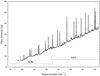 |
Fig. 1 Flux density of Titan in the SSW and SLW spectral bands of SPIRE from the July 16, 2010 observations. |
On July 16, 2010, although the Saturn-Titan separation was large enough to avoid any direct contamination of the Titan spectra by Saturn, the configuration was such that radiation from Saturn entered the instrument through the input port of the SPIRE imaging photometer, resulting in a straylight contribution to the SLW band below 20 cm-1. Therefore, we have subtracted the baseline continuum from the SPIRE spectra and fitted the line contrast in the observed transitions, restricting ourselves to wavenumbers above 20 cm-1. In addition to an extra continuum, a contamination signal from Saturn would produce CH4 absorption lines that would be much broader than the CH4 emission lines on Titan, and be characterized by a depth of about 5% (Swinyard, private communication). The absence of such broad absorption in the SPIRE data indicates that the radiation of Saturn does not affect the CH4 line we observe towards Titan.
In the following, the SLW and SSW spectra are merged into a single spectrum without any adjustment, since the two data sets match each other to within 3 − 4% percent in the overlapping region. A total of 61 emission lines are detected in the SPIRE spectrum, arising from the rotational transitions of the following molecules: CH4 (1 line at 41.9 cm-1), CO (10 lines from J = 4−3 to J = 13−12), 13CO (8 lines from from J = 6−5 to J = 13−12), C18O (same), HCN (12 lines from J = 6−5 to J = 17−16), H13CN (11 lines from J = 7−6 to J = 17−16), and HC15N (same). We note that 16 of these lines appear blended at the resolution of SPIRE, including four CO lines, one C18O line, one HCN line, six H13CN lines, and four HC15N lines.
3. Radiative transfer modeling and results
The model spectra were calculated in units of flux (Jansky) with a line-by-line radiative transfer code accounting for the spherical geometry of Titan’s atmosphere, as described in Marten et al. (2002). For the CO and HCN transitions, we used the intensities from Pickett et al. (1998), and for CH4, those from Boudon et al. (2010). The collisional half-widths at 296 K are respectively 0.060 cm-1 bar-1 (Rothman et al. 2009), 0.060 cm-1 bar-1 (Varanasi et al. 1987; Nakazawa & Tanaka 1982; Hartmann et al. 1988; Dick et al. 2009), and 0.110 cm-1 bar-1 (Yang et al. 2008; Schmidt et al. 1993), and vary with temperature with exponents equal to 0.77, 0.77, and 0.67, respectively.
As regards the temperature structure, we combined the thermal profile retrieved between 140 and 500 km from disk-averaged Cassini-CIRS measurements (Vinatier et al. 2010) with that measured by Huygens-HASI at altitudes below 140 km (Fulchignoni et al. 2005). As for the CO mole fraction, which is not known to vary with altitude, that of CH4 is assumed to be constant with height, since the transitions that we observe are formed between the tropopause and the homopause. For the vertical distribution of HCN, we adopt as an initial guess the result of Marten et al. (2002) obtained from millimetric observations at IRAM, and scale it with a constant factor to fit the observed transitions.
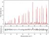 |
Fig. 2 Top – the best-fit model (red line) is compared with the Titan flux spectrum from which the baseline continuum has been subtracted (black line); bottom – (observed spectrum – best-fit model) residuals. |
In the spectral interval that is free of contamination from Saturn (20 to 52 cm-1), we checked that the continuum of the model spectrum agreed with that of the SPIRE spectrum to within 5%, which is similar to the flux calibration uncertainty. To compare with the observed continuum-subtracted SPIRE spectrum, we then subtracted the best-fit continuum from the model spectrum. The best-fit to the SPIRE data was obtained by adjusting the CH4 and CO mole fractions, and the HCN scaling factor, as well as the 12C/13C, 14N/15N, and 16O/18O isotopic ratios. More precisely, the method consisted in finding a minimum in the χ2 calculated from the flux residuals in all of the observed transitions of a given absorber. The error bar associated with each retrieved value was determined by assuming a 5% uncertainty in the flux calibration combined with an intrumental noise estimated at ΔFσ = 0.08 Jy. For the strong CO and HCN lines, the error budget is dominated by the calibration uncertainty, whereas for the weaker lines, in particular those of 13CO and C18O, the instrumental noise is the largest contributor. Figure 2 shows a comparison of the resulting model spectrum with the SPIRE spectrum. All the observed transitions are closely matched by the model, and no unidentified feature is observed above the 3σ noise level.
Figure 3 focuses on a particularly rich portion of the spectrum containing transitions of all seven molecular species investigated here, whereas Fig. 4 shows the simultaneous match obtained for six C18O transitions out of the eight observed. Finally, Table 2 summarizes our results in terms of mole fractions and isotopic ratios.
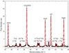 |
Fig. 3 A portion of the SPIRE spectrum (dots with error bars), along with the best-fit model (red line). |
 |
Fig. 4 Simultaneous fits to six of the C18O transitions. |
Retrieved mole fractions and isotopic ratios.
4. Discussion
The molecules whose signatures we observed with SPIRE had been previously detected on Titan. We now compare our results with abundance determinations published so far.
The most recent and precise determinations of the stratospheric abundance of CH4 are those obtained from the Huygens-GCMS experiment (Niemann et al. 2010) – 1.48 ± 0.09% at altitudes of 76 − 140 km – and from the Cassini-CIRS experiment − 1.6 ± 0.5% (Flasar et al. 2005). Our value of 1.33 ± 0.07% is therefore consistent with these previous determinations.
For HCN, since the retrieved scaling factor is very close to unity, our analysis confirms the result of Marten et al. (2002) from whole-disk millimetric observations. A more recent result obtained by Vinatier et al. (2007), using Cassini-CIRS mid-infrared limb spectra, is shown in Fig. 5 along with the one we derived by scaling the Marten et al. (2002) distribution. The CIRS measurements pertain to 15°S latitude, whereas the disk-integrated SPIRE observations are mostly sensitive to the equatorial and mid-latitude regions. This is noteworthy since the concentration of HCN is known to increase towards high northern latitudes. With that slight caveat, we find that the two profiles are in good agreement between 90 and 250 km, the altitude range where HCN contributes most to the SPIRE spectrum.
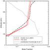 |
Fig. 5 Derived disk-averaged distribution of HCN, compared with the profile obtained by Vinatier et al. (2007) from Cassini-CIRS data at 15°S latitude. Also shown is the contribution function of HCN at 42 cm-1. |
In the case of CO, a direct comparison can be made with the Cassini-CIRS value of 47 ± 8 ppm obtained from the fitting of a dozen rotational lines in the submillimeter range (de Kok et al. 2007a), and with the value of 51 ± 4 ppm found by Gurwell (2004) from observing the (3 − 2) line at 11.53 cm-1. Our value of 40 ± 5 ppm is in good agreement with these previous results.
Quite a few determinations of the 12C/13C ratio on Titan have been published, pertaining to various molecular species, namely CH4, CH3D, C2H2, C2H6, C4H2, CO, CO2, HCN, and HC3N. The value that we derive in CO – 87 ± 6 – agrees with that obtained in the same species by Gurwell (2008) from SMA observations, i.e. 84 ± 6. The value we obtain in HCN – 96 ± 13 − is also consistent with the range of values derived by Gurwell (2004) from SMA observations, i.e. 108 ± 20 or 132 ± 25, depending on the assumed temperature structure, but slightly less so with the value of 75 ± 12 determined by Vinatier et al. (2007) from Cassini-CIRS mid-infrared limb spectra. Despite their interest from the point of view of the chemical evolution of Titan’s atmosphere, a thorough comparison and discussion of the 12C/13C ratio determinations in the various molecular species is beyond the scope of this report. We note, however, that the range of values derived for both CO and HCN includes the Solar System reference value of 89.3 (Lodders 2003), suggesting that no significant carbon fractionation occurred in CO or HCN.
For 14N/15N, Marten et al. (2002) derived a value of 60 − 70, Gurwell (2004) obtained 72 ± 9 or 94 ± 13, depending on the assumed temperature structure, and Vinatier et al. (2007) determined a value of 56 ± 8, all these values pertaining to HCN. Our value of 76 ± 6 is consistent with that of Marten et al., and with the lower value of Gurwell, but it is at odds with his higher value, and with that of Vinatier et al. A ratio of ~ 71 (average of the three consistent values) is about 3.8 times smaller than the terrestrial ratio of 272 (Lodders 2003). Interestingly, a higher ratio – 183 ± 5 – was measured in N2 by the Huygens-GCMS experiment (Niemann et al. 2010). Liang et al. (2007) showed that the different ratios in N2 and HCN can be explained primarily by the photolytic fractionation of 14N14N and 14N15N.
For 16O/18O, the previous determinations are the unpublished result of Gurwell (2008) in CO, i.e. 400 ± 41, and that of Nixon et al. (2008) in CO2, i.e. 346 ± 110. Our value of 380 ± 60 is in-between these two previous values, but the preliminary value of 250 (without error bar) reported by Owen et al. (1999) appears to be in conflict with the above results. Averaging the first three values would give 16O/18O ~ 377, about 1.3 smaller than the terrestrial value of 498.8 (Lodders 2003). We note, however, that the oxygen isotopic ratio may not be the same in CO2 and CO, since CO2 is thought to be produced from exogenic OH (i.e. H2O) by means of the reaction OH + CO → CO2 + H, such that the value in CO2 may be affected by that in H2O. To explain the 18O enrichment first detected by Owen et al. (1999), Wong et al. (2002) hypothesized that CO has a primordial origin with an initial enrichment in both 13CO and C18O. They showed that the initital 13CO enrichment would be diluted over 800 My through isotope-dependent reactions and isotopic exchange reactions, whereas that of C18O would be more preserved. Alternatively, Hörst et al. (2008) and Cassidy & Johnson (2010) proposed that current CO production results from the precipitation of O+ or O in the upper atmosphere of Titan from the Enceladus torus. The Herschel-HIFI observations of the Enceladus torus in water lines, analyzed by Hartogh et al. (2011), confirmed that this scenario is quantitatively viable.
Since the composition of the Enceladus plumes is reminiscent of that of cometary material, it is interesting to compare the 16O/18O Titan value with that measured in comets. In-situ measurements performed by the Giotto spacecraft gave a value of 495 ± 37 for H2O in comet 1P/Halley (Eberhardt et al. 1995), whereas remote sensing of submillimetric H O lines from the satellite Odin resulted in values ranging from 508 ± 33 to 550 ± 75 in four Oort-Cloud comets (Biver et al. 2007), and ultraviolet observations yielded a value of 425 ± 55 in OH for comet C/2002 T7 (LINEAR) (Hutsemékers et al. 2008). Since all these values are consistent with the terrestrial ratio, it would premature to draw conclusions. Measuring the 16O/18O ratio in the Enceladus plumes would, however, provide a strong constraint on the origin of the non-terrestrial Titan ratio.
Acknowledgments
SPIRE has been developed by a consortium of institutes led by Cardiff Univ. (UK) and including Univ. Lethbridge (Canada); NAOC (China); CEA, LAM (France); IFSI, Univ. Padua (Italy); IAC (Spain); Stockholm Observatory (Sweden); Imperial College London, RAL, UCL-MSSL, UKATC, Univ. Sussex (UK); Caltech, JPL, NHSC, Univ. Colorado (USA). This development has been supported by national funding agencies: CSA (Canada); NAOC (China); CEA, CNES, CNRS (France); ASI (Italy); MCINN (Spain); SNSB (Sweden); STFC (UK); and NASA (USA).
References
- Anderson, C. M., & Samuelson, R. E. 2011, Icarus, 212, 762 [NASA ADS] [CrossRef] [Google Scholar]
- Biver, N., Bockelée-Morvan, D., Crovisier, J., et al. 2007, Planet. Space Sci., 55, 1058 [NASA ADS] [CrossRef] [Google Scholar]
- Bjoraker, G., Achterberg, R., Anderson, C., et al. 2008, BAAS, 40, 448 [NASA ADS] [Google Scholar]
- Boudon, V., Pirali, O., Roy, P., et al. 2010, J. Quant. Spec. Radiat. Transf., 111, 1117 [Google Scholar]
- Cassidy, T. A., & Johnson, R. E. 2010, Icarus, 209, 696 [Google Scholar]
- Courtin, R. 1982, Icarus, 51, 466 [NASA ADS] [CrossRef] [Google Scholar]
- de Kok, R., Irwin, P. G. J., Teanby, N. A., et al. 2007a, Icarus, 186, 354 [NASA ADS] [CrossRef] [Google Scholar]
- de Kok, R., Irwin, P. G. J., Teanby, N. A., et al. 2007b, Icarus, 191, 223 [NASA ADS] [CrossRef] [Google Scholar]
- Dick, M. J., Drouin, B. J., Crawford, T. J., & Pearson, J. C. 2009, J. Quant. Spec. Radiat. Transf., 110, 628 [NASA ADS] [CrossRef] [Google Scholar]
- Eberhardt, P., Reber, M., Krankowsky, D., & Hodges, R. R. 1995, A&A, 302, 301 [NASA ADS] [Google Scholar]
- Flasar, F. M., Achterberg, R. K., Conrath, B. J., et al. 2005, Science, 308, 975 [NASA ADS] [CrossRef] [Google Scholar]
- Fulchignoni, M., Ferri, F., Angrilli, F., et al. 2005, Nature, 438, 785 [NASA ADS] [CrossRef] [Google Scholar]
- Griffin, M. J., Abergel, A., Abreu, A., et al. 2010, A&A, 518, L3 [Google Scholar]
- Gurwell, M. A. 2004, ApJ, 616, L7 [NASA ADS] [CrossRef] [Google Scholar]
- Gurwell, M. A. 2008, BAAS, 40, 423 [NASA ADS] [Google Scholar]
- Gurwell, M. A., Moullet, A., & the eSMA Team 2009, BAAS, 41, #30.07 [Google Scholar]
- Hartmann, J. M., Rosenmann, L., Perrin, M. Y., & Taine, J. 1988, Appl. Opt., 27, 3058 [NASA ADS] [CrossRef] [Google Scholar]
- Hartogh, P., Lellouch, E., Crovisier, J., et al. 2009, Planet. Space Sci., 57, 1596 [NASA ADS] [CrossRef] [Google Scholar]
- Hartogh, P., Lellouch, E., Moreno, R., et al. 2011, A&A, 532, L2 [NASA ADS] [CrossRef] [EDP Sciences] [Google Scholar]
- Hidayat, T., Marten, A., Biraud, Y., & Moreno, R. 2002, in 8th Asian-Pacific Regional Meeting, Volume II, ed. S. Ikeuchi, J. Hearnshaw, & T. Hanawa, 9 [Google Scholar]
- Hörst, S. M., Vuitton, V., & Yelle, R. V. 2008, J. Geophys. Res. (Planets), 113, E10006 [Google Scholar]
- Hutsemékers, D., Manfroid, J., Jehin, E., Zucconi, J.-M., & Arpigny, C. 2008, A&A, 490, L31 [NASA ADS] [CrossRef] [EDP Sciences] [Google Scholar]
- Liang, M.-C., Heays, A. N., Lewis, B. R., Gibson, S. T., & Yung, Y. L. 2007, ApJ, 664, L115 [NASA ADS] [CrossRef] [Google Scholar]
- Lodders, K. 2003, ApJ, 591, 1220 [NASA ADS] [CrossRef] [Google Scholar]
- Marten, A., Hidayat, T., Biraud, Y., & Moreno, R. 2002, Icarus, 158, 532 [NASA ADS] [CrossRef] [Google Scholar]
- Moreno, R., Lellouch, E., Hartogh, P., et al. 2010, BAAS, 42, 1088 [NASA ADS] [Google Scholar]
- Moreno, R., Lellouch, E., Lara, L. M., et al. 2011, A&A, accepted [Google Scholar]
- Nakazawa, T., & Tanaka, M. 1982, J. Quant. Spec. Radiat. Transf., 28, 409 [Google Scholar]
- Niemann, H. B., Atreya, S. K., Demick, J. E., et al. 2010, J. Geophys. Res. (Planets), 115, E12006 [NASA ADS] [CrossRef] [Google Scholar]
- Nixon, C. A., Jennings, D. E., Bézard, B., et al. 2008, ApJ, 681, L101 [NASA ADS] [CrossRef] [Google Scholar]
- Owen, T., Biver, N., Marten, A., Matthews, H., & Meier, R. 1999, IAU Circ., 7306, 3 [NASA ADS] [Google Scholar]
- Pilbratt, G. L., Riedinger, J. R., Passvogel, T., et al. 2010, A&A, 518, L1 [CrossRef] [EDP Sciences] [Google Scholar]
- Pickett, H. M., Poynter, R. L., Cohen, E. A., et al. 1998, J. Quant. Spec. Radiat. Transf., 60, 883 [Google Scholar]
- Rengel, M., Sagawa, H., & Hartogh, P. 2010, in Advances in Geosciences, ed. A. Bhardwaj (Singapore: World Scientific), 25, 173 [Google Scholar]
- Rothman, L. S., Gordon, I. E., Barbe, A., et al. 2009, J. Quant. Spec. Radiat. Transf., 110, 533 [Google Scholar]
- Schmidt, C., Populaire, J. C., Walrand, J., Blanquet, G., & Bouanich, J. P. 1993, J. Mol. Spectrosc., 158, 423 [NASA ADS] [CrossRef] [Google Scholar]
- SPIRE Observers Manual v2.2, Herschel Science Centre, HERSCHEL-HSC-DOC-0789 accessed from http://herschel.esac.esa.int/Docu-mentation.shtml [Google Scholar]
- Swinyard, B. M., Ade, P., Baluteau, J.-P., et al. 2010, A&A, 518, L4 [Google Scholar]
- Teanby, N. A., Irwin, P. G. J., de Kok, R., & Nixon, C. A. 2010, Faraday Discussions, 147, 51 [Google Scholar]
- Varanasi, P., Chudamani, S., & Kapur, S. 1987, J. Quant. Spec. Radiat. Transf., 38, 167 [Google Scholar]
- Vinatier, S., Bézard, B., & Nixon, C. A. 2007, Icarus, 191, 712 [NASA ADS] [CrossRef] [Google Scholar]
- Vinatier, S., Bézard, B., Nixon, C. A., et al. 2010, Icarus, 205, 559 [NASA ADS] [CrossRef] [Google Scholar]
- Wong, A.-S., Morgan, C. G., Yung, Y. L., & Owen, T. 2002, Icarus, 155, 382 [NASA ADS] [CrossRef] [Google Scholar]
- Yang, C., Buldyreva, J., Gordon, I. E., et al. 2008, J. Quant. Spec. Radiat. Transf., 109, 2857 [NASA ADS] [CrossRef] [Google Scholar]
All Tables
All Figures
|
Fig. 1 Flux density of Titan in the SSW and SLW spectral bands of SPIRE from the July 16, 2010 observations. |
| In the text | |
|
Fig. 2 Top – the best-fit model (red line) is compared with the Titan flux spectrum from which the baseline continuum has been subtracted (black line); bottom – (observed spectrum – best-fit model) residuals. |
| In the text | |
|
Fig. 3 A portion of the SPIRE spectrum (dots with error bars), along with the best-fit model (red line). |
| In the text | |
|
Fig. 4 Simultaneous fits to six of the C18O transitions. |
| In the text | |
|
Fig. 5 Derived disk-averaged distribution of HCN, compared with the profile obtained by Vinatier et al. (2007) from Cassini-CIRS data at 15°S latitude. Also shown is the contribution function of HCN at 42 cm-1. |
| In the text | |
Current usage metrics show cumulative count of Article Views (full-text article views including HTML views, PDF and ePub downloads, according to the available data) and Abstracts Views on Vision4Press platform.
Data correspond to usage on the plateform after 2015. The current usage metrics is available 48-96 hours after online publication and is updated daily on week days.
Initial download of the metrics may take a while.