| Issue |
A&A
Volume 536, December 2011
|
|
|---|---|---|
| Article Number | A35 | |
| Number of page(s) | 14 | |
| Section | Extragalactic astronomy | |
| DOI | https://doi.org/10.1051/0004-6361/201117834 | |
| Published online | 05 December 2011 | |
Optically faint radio sources: reborn AGN?
1
Centro de Astrofísica da Universidade do Porto, Rua das Estrelas, 4150–762 Porto, Portugal
e-mail: This email address is being protected from spambots. You need JavaScript enabled to view it.
2
Leiden Observatory, University of Leiden, PO Box 9513, 2300 RA Leiden, The Netherlands
3
Departamento de Física e Astronomia, Faculdade de Ciências da Universidade do Porto, Rua do Campo Alegre 687, 4169–007 Porto, Portugal
4 Centro de Investigação em Ciências Geo-Espaciais, Faculdade de Ciências da Universidade do Porto, Porto, Portugal
5 SIM, Faculdade de Ciências da Universidade de Lisboa, Lisboa, Portugal
Received: 5 August 2011
Accepted: 26 September 2011
Abstract
We present our discovery of several relatively strong radio sources in the field-of-view of SDSS galaxy clusters that have no optical counterparts down to the magnitude limits of the SDSS. The optically faint radio sources appear as double-lobed or core-jet objects in the FIRST radio images and have projected angular sizes ranging from 0.5 to 1.0 arcmin. We followed-up these sources with near-infrared imaging using the wide-field imager HAWK-I on the VLT. We detected Ks-band emitting regions, about 1.5 arcsec in size and coincident with the centers of the radio structures, in all sources, with magnitudes in the range 17–20 mag. We used spectral modelling to characterize the sample sources. In general, the radio properties are similar to those observed in 3CRR sources but the optical-radio slopes are consistent with those of moderate to high redshift (z < 4) gigahertz-peaked spectrum sources. Our results suggest that these unusual objects are galaxies whose black hole has been recently re-ignited but that retain large-scale radio structures, which are signatures of previous AGN activity.
Key words: galaxies: active
© ESO, 2011
1. Introduction
In the past fifteen years, deep and extensive radio observations of the Hubble Deep Field (HDF; Richards et al. 1999), and surveys such as the Very Large Array (VLA) 8.4 GHz survey (Fomalont et al. 2002), Phoenix (Hopkins et al. 2003), and Atlas (Norris et al. 2006) have uncovered a number of previously uncatalogued radio sources. These are characterized by flux densities that range from several microjansky to hundreds of millijansky and by projected angular sizes that can be as large as several megaparsecs. Cross-correlation studies have shown that as many as 10–15% of the compact radio sources have faint or no optical or infrared counterparts (Hopkins et al. 2003; Sullivan et al. 2004; Higdon et al. 2005, 2008; Middelberg et al. 2008a; Garn & Alexander 2008; Huynh et al. 2010; Norris et al. 2011; Banfield et al. 2011; Zinn et al. 2011; see also Machalski et al. 2001; Rigby et al. 2007). While a significant fraction of the sub-millijansky radio population appears to be faint star-forming galaxies (e.g. Haarsma et al. 2000), radio sources that are faint in the optical or infrared are generally consistent with high redshift (z > 1), radio-loud sources or quasars (Higdon et al. 2005, 2008; Garn & Alexander 2008; Jarvis et al. 2009; Huynh et al. 2010; Norris et al. 2011; Banfield et al. 2011).
Radio data.
To study and establish the link between active galactic nuclei (AGN) and cluster properties, we have compiled a sample of Sloan Digital Sky Survey (SDSS) maxBCG clusters, at redshifts between 0.17 and 0.28, that contain radio sources located in projection onto their cores. Surprisingly, we have discovered a number of relatively strong radio sources in some of the cluster fields that have no optical counterparts. There are eight such sources, seven of which have FR II-type (Fanaroff & Riley 1974) and one of which has a core-jet-type radio morphology in the Faint Images of the Radio Sky at Twenty Centimeter (FIRST; White et al. 1997) maps. These radio sources possess angular sizes of 0.5–1 arcmin and flux densities of 1–80 mJy. They have not been identified at any other wavelengths according to our data mining in the NASA IPAC Extragalactic Database (NED) and all databases available through the Virtual Observatory (VO).
Follow-up deep, near-infrared (NIR) observations were obtained with the wide-field imager HAWK-I at the European Southern Observatory (ESO) Very Large Telescope (VLT) to try to identify the radio source host galaxy. In this paper, we present the data and discuss the nature of these objects, based mainly on their spectral energy distribution (SED) and spectral modelling.
The paper is organised as follows. Section 2 describes the sample selection, Sect. 3 presents the new observations and data reduction, and Sect. 4 describes the SDSS and Stripe 82 component identifications. In Sect. 5, we discuss the SED of the objects and their nature. We summarise our conclusions in Sect. 6.
Throughout the paper, we have assumed the seven year Wilkinson Anisotropy Probe (WMAP7) cosmological parameter set for a flat Universe, H0 = 70 km s-1 Mpc-1 and Ωm = 0.27 (Larson et al. 2011).
2. Sample selection
The SDSS maxBCG cluster catalog (13 823 clusters; Koester et al. 2007) was used as the seed catalogue for our study. The radio sources were selected in the following manner:
-
we first cross-correlated the cluster sample with the FIRSTcatalogue (White et al. 1997);
-
we then retained 291 clusters that contained at least one FIRST object within 1 Mpc in projection from the brightest cluster galaxy (BCG);
-
a visual inspection of the selected fields provided a subsample of radio galaxies with extended double-lobed or core-jet radio morphology;
-
for these, when a secure SDSS identification was made, the existing spectroscopy or multi-band photometry was used to optically characterise the source and assess whether the source belongs to the cluster or not.
During this process, we identified eight radio sources with no optical SDSS counterpart, which indicates that their rAB-band magnitudes must be fainter than 22 mag. The radio sources are located in the fields-of-view of clusters with redshifts ranging from 0.17 to 0.28. The radio sources are characterized by their radio-loudness (as defined by a large radio flux density relative to the optical and NIR; see Sects. 5.2 and 5.3), arcsec-scale FR II-type, or core-jet radio morphology and relatively strong FIRST flux densities in the range 1 mJy < F1.4 GHz < 80 mJy.
Table 1 contains the radio data for the sample sources. Radio sources are identified by the sequential number of the cluster field to which they belong in projection, as it appears in the maxBCG cluster catalogue (Koester et al. 2007). Radio source components are identified based on their position and nature relative to the overall radio source structure. For the only core-jet radio source in our sample (maxBCG 3131; Fig. 1), we have designated the radio emission regions North Comp and South Comp 1 and 2 (Table 1). In addition, maxBCG 2596 is the only radio source with a radio core detection (Nucleus; Table 1). We note that the radio properties of the optically faint radio sources are dominated by the extended (lobe) radio emission.
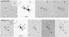 |
Fig. 1 From left to right, inverted greyscale image of the NIR emission, FIRST greyscale emission with superimposed radio contours, the first two levels of the FIRST contour plots superimposed on the NIR field and likewise superimposed on the SDSS and the Stripe 82 (maxBCG 3131) rAB-band field. The field numbers are the sequential numbers of SDSS macxBCG cluster fields to which the radio sources belong, as they appear in Koester et al. (2007), letters/numbers are the NIR components and lobe designations refer to the radio components. The inlays contain the NIR N component (Tables 3 and 4), coincident with the center of the radio structure. Radio contours are: (top) 0.001, 0.002, 0.004, 0.008 mJy; (bottom) 0.001, 0.002, 0.004, 0.008 mJy. |
SDSS maxBCG cluster redshifts.
Table 2 contains redshift information about the maxBCG clusters containing our sample sources in their field-of-view.
3. Near-infrared observations and data reduction
The unidentified radio sources were followed-up with NIR imaging using the wide-field imager HAWK-I on the ESO UT4 of the VLT. The proposal, with reference 081.A-0624(A), was awarded a total of 2.7 h observing time during period 81. The total integration time on-source was about 1000 s. The data were reduced using the HAWK-I data reduction pipeline (version 1.4.2), which includes recipes for darks, flats, zero-point computation, detector linearity, illumination, additional calibration, distortion corrections, jittering and image stitching. The reduced images were then astrometrically calibrated using the Two Micron All Sky Survey (2MASS) catalogue and tools provided in the Graphical Astronomy and Image Analysis Tool (GAIA; version 4.3–0). The astrometric calibration is good to better than one arcsec, which is sufficient for our purposes. Aperture photometry was performed on the images using the GAIA sextractor program. The Ks-band magnitudes (in the Vega magnitude system) were estimated using zero-points given in the corresponding quadrant of the standard star images and assuming no significant color term with respect to 2MASS (ESO HAWK-I Science Verification, November 7, 2007: Note on Photometry1).
Near-infrared data.
Optical data.
Results of the NIR observations are presented in Table 3. The NIR sources are identified by the sequential number of the cluster field to which they belong in projection, as it appears in the maxBCG cluster catalogue (Koester et al. 2007). The NIR counterparts of the centers of the radio structures are designated as components “N”. The typical sizes of these central NIR components, as provided by GAIA sextractor aperture photometry, are ~1.5 arcsec. For the special case of maxBCG 8495, we used GAIA manual aperture photometry to estimate the magnitude in a region (~2 arcsec) containing the “double nuclear” sources Na and Nb (component N; Table 3). The NIR sources near or within (in projection) but not associated with (see Sect. 5.1) the FIRST radio sources, are identified based on their position relative to the overall radio source structure. The quoted NIR magnitudes are in the Vega magnitude system.
4. SDSS and Stripe 82 data
The SDSS (York et al. 2000) is a survey covering more than 35% of the sky providing deep, photometric observations in 5 bands (u, g, r, i and z; AB magnitude system) of about 500 million objects and spectra for more than 1 million sources.
We used the SDSS Data Release 7 (DR7; Abazajian et al. 2009) to attempt to identify optical counterparts of the radio and NIR components of our sources. Identification was based on the coincidence of the positions to less than 1 arcsec, followed by visual inspection of the images. None of the radio components (Table 1) or NIR emission regions coincident with the centers of the radio structures (components N; Table 3) were detected in the SDSS, providing an rAB-band upper limit of ~22 mag. However, several NIR sources near or within (in projection) but not associated with (see Sect. 5.1) the FIRST radio sources, were identified.
Stripe 82 is a ~300 deg2 region along the celestial equator, that has been imaged by a number of different collaborations (with the same set-up and in the same bands) over one hundred times, providing coadded optical data two magnitudes deeper than the single-epoch SDSS data.
Three of our fields are located within the Stripe 82 region, namely maxBCG 3131, maxBCG 6167, and maxBCG 8495. For these fields, we searched for possible optical counterparts to our NIR components. Identification was based on the visual inspection of all possible counterparts within 5 arcsec of the NIR source. For each of the three fields, we detected the faint optical Stripe 82 counterparts of the NIR components coincident with the centers of the radio structures (components N; Table 3). We have identified the Stripe 82 optical counterparts to several other NIR sources near or within (in projection) but not associated with (see Sect. 5.1) the FIRST radio sources.
Stripe 82 optical counterparts were also sought directly for the extended radio components. In this procedure, Stripe 82 yielded matches within 5 arcsec of the positions of the radio components in maxBCG 3131 and maxBCG 6167. For maxBCG 3131, radio components North Comp and South Comp 1 coincide with the position of optical sources; these are rather faint (rAB-band magnitudes of 22.7 and 23.7 mag) extended sources. As for maxBCG 6167, only its North Lobe radio component flags a cross-match in Stripe 82; this is an extremely faint extended object with an ill-determined rAB-band magnitude of 24.5 ± 1.5 mag. Because radio lobes are not expected to produce significant optical emission, these cross-matches are most likely chance alignments of galaxies unassociated with our radio sources, that are located along the same line-of-sight of the radio structure.
The faintness of the optical counterparts in the Stripe 82 data prevents us from deriving structural indicators for the galaxies.
The results of the cross-correlation with the SDSS and Stripe 82 data are included in Table 4. The optical magnitudes are in the AB magnitude system.
5. Discussion
5.1. Individual sources
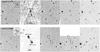 |
Fig. 2 From left to right, inverted greyscale image of the NIR emission, FIRST greyscale emission with superimposed radio contours, the first two levels of the FIRST contour plots superimposed on the NIR field and likewise superimposed on the SDSS field and the Stripe 82 (maxBCG 6167 and 8495) rAB-band field. The field numbers are the sequential numbers of SDSS macxBCG cluster fields to which the radio sources belong as they appear in Koester et al. (2007), letters/numbers are the NIR components and lobe designations refer to the radio components. The inlays contain the NIR N component (Tables 3 and 4), coincident with the center of the radio structure. Radio contours are: (top) 0.0004, 0.0008, 0.0016 mJy (in log); (bottom) 0.0005, 0.0010, 0.0020, 0.0040, 0.0060, 0.0080 mJy. |
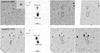 |
Fig. 3 From left to right, inverted greyscale image of the NIR emission, FIRST greyscale emission with superimposed radio contours, the first two levels of the FIRST contour plots superimposed on the NIR field and likewise superimposed on the SDSS rAB-band field. The field numbers are the sequential numbers of SDSS macxBCG cluster fields to which the radio sources belong, as they appear in Koester et al. (2007), letters/numbers are the NIR components and lobe designations refer to the radio components. The inlays contain the NIR N component (Tables 3 and 4), coincident with the center of the radio structure. Radio contours are: (top) 0.001, 0.002, 0.004, 0.008, 0.016 mJy; (bottom) 0.008, 0.0016, 0.0032, 0.0064, 0.0128, 0.0256, 0.0512 mJy. |
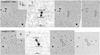 |
Fig. 4 From left to right, inverted greyscale image of the NIR emission, FIRST greyscale emission with superimposed radio contours, the first two levels of the FIRST contour plots superimposed on the NIR field and likewise superimposed on the SDSS rAB-band field. The field numbers are the sequential numbers of SDSS macxBCG cluster fields to which the radio sources belong, as they appear in Koester et al. (2007), letters/numbers are the NIR components and lobe designations refer to the radio components. The inlays contain the NIR N component (Tables 3 and 4), coincident with the center of the radio structure. Radio contours are: (top) 0.0004, 0.0008, 0.0016, 0.0032 mJy (in log); (bottom) 0.0005, 0.0010, 0.0020, 0.0040, 0.0080 mJy. |
The FIRST, NIR, SDSS, and Stripe 82 (when available) rAB-band images of the fields containing the sample sources are presented in Figs. 1–4. The HAWK-I observations were successful, as NIR emission, coincident with the centers of the radio structures (components N; Table 3), was detected in all the targets. In the particular case of maxBCG 2596, the central NIR emission source (component N; Table 3) coincides with the radio core (Nucleus; Table 1), while in maxBCG 3131, the central NIR source (component N; Table 3) falls between the radio components North Comp and South Comp 1 (Table 1). We also investigated all NIR sources near or within (in projection) but not associated with the FIRST radio sources. In the following, we discuss the HAWK-I sources individually:
maxBCG 2596. In this object, we identified the NIR counterpart (component N; Table 3) to the radio core (Nucleus; Table 1) at the center of the radio structure, which is the brightest NIR component in our sample but still falls below the ~22 mag rAB-band limit of the SDSS. We also detected NIR sources (components W and E; Table 3) coincident with the termination of the radio lobes (components East and West Lobe; Table 1), the latter of which display extended NIR morphology. The NIR E and W components are detected in the SDSS image, where they are identified with extended, galaxy-type objects – J010202.12-103258.3 and J010159.33-103311.2 (Table 4) – with somewhat similar rAB-band magnitudes of ~19.4 and ~20.9 (Table 4), but distinct photometric redshifts (z = 0.09 and 0.19; Table 4). Because radio lobes do not produce significant amounts of optical emission and owing to the redshift discrepancy between the radio source (z = 0.56; Table 7; see also Sect. 5.3) and the corresponding optical/NIR components (z = 0.09 and 0.19; Table 4), we conclude that this is a chance alignment. However, according to their redshifts, the NIR E component lies in the cluster foreground, whereas the SDSS counterpart identified with the NIR W component has a photometric redshift (z = 0.19; Table 4) consistent with both the photometric redshift of the cluster field determined by Koester et al. (2007) and the spectroscopic redshift of the BCG associated with the same cluster (z ~ 0.18; Table 2). One can conclude that, if this cross-identification is correct, then the NIR W component is embedded in the cluster and, consistently, has a g − r color index typical of an early-type galaxy (Fukugita et al. 1995) at the cluster distance (z ~ 0.18; Table 2).
maxBCG 3131. The HAWKI-I image shows that this object has a complex NIR morphology. All of the NIR components can be identified on the Stripe 82 images with rAB-band magnitudes ranging from 19 to 24 mag (Table 4). The central NIR source (component N; Table 3), coincident with the center of the radio structure (between North Comp and South Comp 1 components; Table 1) is the faintest, with a very blue g − r = 0.35 color index, consistent with the optical color of a quasar (Richards et al. 2001) at the estimated redshift of our radio source (z = 1.03; Table 7; see also Sect. 5.3). This result is confirmed by the photometric redshift estimate for the Stripe 82 detection (z = 1.57; Table 7; see also Sect. 5.3). There is diffuse NIR emission to the east (components E1, E2, and E3; Table 3), coincident with the outline of the northern radio component (component North Comp; Table 1). From careful inspection of the Stripe 82 images, it can be seen that components E1 and E2 are two resolved components of the same edge-on foreground galaxy (relative to the cluster in this field), located at a redshift of z ~ 0.08 (Table 4; as indicated by the SDSS photometric redshift of component E2). Component E3 (Table 3) is identified with the rAB-band 21.8 mag SDSS extended galaxy-type source J003448.99-002130.9 (Table 4), located at a photometric redshift of z = 0.58 (Table 4), which is higher than the one attributed to the cluster dominating the field-of-view (z = 0.27; Table 2), but closer than our radio source estimate (z = 1.03; Table 7; see also Sect. 5.3). Extended NIR galaxy-type emission is also present due south (components S1 and S2; Table 3) of the southern radio components (components South Comp 1 and 2; Table 1) and identified with rAB-band ~21–23 mag Stripe 82 sources – J003447.51-002145.2 and J003447.21-002145.5 (Table 4) – the former being located at a higher redshift (z = 0.46; Table 4) than the one attributed to the cluster (z = 0.27; Table 2), but still not coinciding, by far, with the estimated redshift of our radio source (z = 1.03; Table 7; see also Sect. 5.3). Furthermore, there are points of aligned southeast-northwest NIR emission perpendicular to the orientation of the radio structure – components D1 and D2 (Table 3). There is a rAB-band ~23 mag Stripe 82 stellar-like identification of component D1 – J003448.41-002136.0 (Table 4) – and a ~21 mag SDSS identification of component D2 – J003447.71-002126.9 (Table 4) – an extended galaxy-type object with a photometric redshift of z ~ 0.60 (Table 4), placing it in the background of the cluster (z = 0.27; Table 2), but at a similar redshift to component E3 (z = 0.58; Table 4). There is also evidence of faint NIR emission (component L; Table 3) within (in projection) the northern radio component (component North Comp; Table 1), which has been identified with a rAB-band ~23 mag stellar-like object in Stripe 82 (Table 4).
maxBCG 6167. As in the case of its radio emission, the NIR emission associated with this source is faint. We detect central NIR emission (component N; Table 3) coincident with the center of the radio structure. An optical counterpart was detected in Stripe 82 – J002452.65-005201.7 (Table 4) – as a galaxy-type source with an rAB-band magnitude of about 25 mag (Table 4). This is the faintest radio, NIR, and optical (Stripe 82) source in our sample. Its extreme g − r blue color of − 0.44 is affected by large magnitude errors (~0.4 mag in each of the 2 bands), rendering it too blue, even for the expected values of a quasar (Richards et al. 2001) at the estimated redshift of our radio source (z=1.13; Table 7; see also Sect. 5.3). This result is confirmed by the photometric redshift estimate for the Stripe 82 detection (z = 1.00; Table 7; see also Sect. 5.3).
maxBCG 8495. The NIR image shows a “double nuclear” emission region (components Na and Nb; Table 3) at the center of the radio structure. A similarly extended galaxy-type morphology is seen in the Stripe 82 image, although Stripe 82 identifies a sole, quite faint, component – J004359.47+001230.4 (Table 4) – with an rAB-band magnitude of about 24 mag and g − r = 1.31 (Table 4). Given its red color and the estimated redshift of the radio source (z = 0.96; Table 7; see also Sect. 5.3), we can conclude that the Stripe 82 optical counterpart has a g − r color index consistent with that of a late-type spiral galaxy (Fukugita et al. 1995), which is coherent with its disky appearance in the NIR. The red color generally excludes a quasar host (Richards et al. 2001) at the estimated redshift of our radio source (z = 0.96; Table 7; see also Sect. 5.3). These results are confirmed by the photometric redshift estimate for the Stripe 82 detection (z = 0.88; Table 7; see also Sect. 5.3). There is also a small patch of unidentified NIR emission (component D; Table 3) near (in projection) to the center of the radio source.
maxBCG 10942. There is a central NIR emission region (component N; Table 3) that is coincident with the center of the radio structure and some unidentified NIR emission to the west (component W; Table 3) of the northern radio lobe (component North Lobe; Table 1), in projection.
maxBCG 11079. This source shows a complex, faint NIR morphology. There is evidence of central NIR emission (component N; Table 3) coincident with the center of the radio structure, which has a disk-like appearance. There are also peaks of unidentified NIR emission within (in projection) and/or near the edge of the southern (components S1, S2 and S3; Table 3) and northern radio lobes (component L; Table 3).
maxBCG 11390. There is a clear NIR detection (component N; Table 3) at the position of the center of the radio structure and an unidentified NIR eastern (component E; Table 3) source.
maxBCG 11780. There is an unidentified region of NIR emission within (in projection) the northern radio lobe (component L; Table 3) and at the position of the center of the radio structure (component N; Table 3).
All the NIR images reveal central emission, relative to the radio structure (components N; Table 3), that we interpret as thermal host-related emission (see Sect. 5.2). The NIR magnitudes of these sources are in the range 17–20 mag (Table 3) and their NIR sizes, provided by GAIA sextractor aperture photometry, are typically ~ 1.5 arcsec. We detect unassociated (relative to the radio source) NIR emission in seven of the eight sources. Some were identified with stars, some with background or cluster galaxies, and still others remain to be identified (Table 4). With the possible exception of maxBCG 2596 NIR component W (Table 4), none of the optically identified NIR components are cluster members.
5.2. Near-infrared-radio correlation
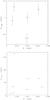 |
Fig. 5 The NIR versus 1.4 GHz FIRST flux density. The NIR flux pertains to the Ks-band fluxes of the NIR components (components N; Table 3) coincident with the radio structure centers. The NIR magnitudes are in the Vega system. The radio core flux density (top) pertains to the radio “core” flux density (Table 6) estimated using funtools on circular regions of approximately the same size (~2 arcsec) and centered on the NIR emission regions N (Table 3; see Sect. 5.2). The total radio flux density (bottom) pertains to the total FIRST flux density as a sum of the flux density of all the FIRST components (Table 1). The errorbar associated with the FIRST flux density corresponds to 1 × rms, where rms is the root mean square, a measure of the noise level in the FIRST image. |
We present, in Fig. 5 (see also Table 6), a plot of the NIR emission versus the FIRST flux density. With the exception of the maxBCG 8495 component N (Table 3; see Sect. 3), the plotted NIR flux (in the Vega magnitude system) corresponds to GAIA sextractor aperture photometry of the NIR components coincident with the radio structure centers (components N; Table 3). Total radio flux densities were calculated as the sum of the flux densities of all the FIRST radio components (Table 1). We note in passing that the extended radio emission dominates the total radio flux density in all of our sources even when we detect a radio core (maxBCG 2596) or core-jet (maxBCG 3131) source. We estimated a radio “core” flux density by applying saoimage ds9 (version 5.1) funtools2 to circular regions of approximately the same size (~2 arcsec) and centered on the NIR emission regions N (Table 3). The radio “core” flux density for sources maxBCG 6167, 8495, and 11390 falls below the 3 × rms (root mean square, as a measure of the noise level) given in the corresponding FIRST images.
Correlation statistics.
We performed two correlation tests on the data – the generalized Kendall’s τ correlation coefficient estimation (BHK) and the estimate of the correlation probability using Cox’s proportional hazard model (Cox-Hazard), as implemented in IRAF (version 2.14.1; Table 5). Both the BHK and Cox-Hazard tests show a > 50% (radio core flux density) and > 80% (total radio flux density) probability that there is no correlation between the FIRST and NIR emission. On these scales and given the radio morphology, the FIRST radio emission corresponds to synchrotron emission associated with the AGN. The lack of correlation between the radio and the NIR emission therefore reflects the thermal nature of the NIR source, which probably originates from the host galaxy. This is in contrast to 3CR galaxies (Spinrad 1985), which commonly have non-thermal NIR central regions associated with the AGN (Baldi et al. 2010).
The infrared-radio correlation, represented by the parameter q, is an indicator of the dominant emission mechanism in a galaxy (Yun et al. 2001); an AGN contribution causes, in general, a decrease in the value of q. Empirically, it has been shown that starburst-dominated galaxies at redshifts below 2 typically have a ratio of about q ~ 1 (Appleton et al. 2004) and q ~ 2.4 (Yun et al. 2001), where  and IR (infrared) is measured at 24 μm and a combination of 60 and 100 μm, respectively. A clear enhancement in the radio emission relative to a pure starburst galaxy is generally attributed to the presence of an AGN. We note that for typical galaxy starburst, AGN, and composite SEDs (e.g. Huynh et al. 2010), the difference between the 24 μm and 2.2 μm flux may be as high as two orders of magnitude. Therefore, in the very extreme case, for a starburst-driven galaxy q ~ − 1.0 in Ks-band.
We proceeded to estimate the infrared-radio correlation using the Ks-band magnitude of the NIR N components (Table 3) and the radio “core” and total radio flux densities, as defined above. The results are contained in Table 6. Our sources show values that are generally consistent with the presence of an AGN (q < 0), with maxBCG 11079 being the most “AGN-dominated” source in the terms of the infrared-radio ratio.
Infrared-radio correlation.
5.3. The spectral energy distribution
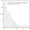 |
Fig. 6 The redshift distribution of the 3CRR (solid line) and GPS (dashed line) sample. |
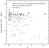 |
Fig. 7 The redshift versus largest linear size (LLS) for the 3CRR (crosses), GPS (triangles), and our sample (circles). The LLS for the GPS sources were obtained from O’Dea & Baum (1997), when a measurement was available. |
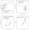 |
Fig. 8 Clockwise from the top left: the redshift versus the 5 GHz power for the 3CRR (crosses), GPS (triangles), and our sample total (closed circles) and core (open circles); the largest linear size (LLS) versus the 5 GHz power for the 3CRR (crosses), GPS (triangles), and our sample total (closed circles) and core (open circles); the redshift versus the K- (GPS and 3CRR) or Ks-band (our sample) magnitude for the 3CRR (crosses), GPS (triangles), and our sample (circles); the K- (GPS and 3CRR) or Ks-band (our sample) magnitude versus the 5 GHz power for the 3CRR (crosses), GPS (triangles), and our sample total (closed circles) and core (open circles). The radio measurements for the 3CRR sample are those of the radio cores, and for the GPS sample it is the total radio power. For our sample, we include the radio “core” power (open circles; Table 7) estimated using funtools in circular regions of approximately the same size (~2 arcsec) and centered on the NIR emission regions N (Table 3; see Sect. 5.2) and the total radio power (closed circles; Table 7), the sum of the power of all the FIRST components (Table 1). We assumed a flat radio spectrum for all sources in order to normalize to 5 GHz. The LLS for the GPS sample were derived from O’Dea & Baum (1997), when a measurement was available. The 3CRR K-band magnitudes are aperture- and emission-line-corrected measurements for a subset of 3CRR sources. For the GPS sample, the K-band magnitudes were obtained by interpolation from NED NIR photometric points. NIR magnitudes for our sample are for the central NIR component, coincident with the center of the radio structure (components N; Table 3). The NIR magnitude system is Vega. |
At first glance, the radio morphologies (Figs. 1–4) suggest that our optically faint radio sources may be similar to the radio sources found in the Third Cambridge Revised Catalogue of Radio Sources (3CRR) 3. We present in Figs. 6–8 plots of the redshift, LLS, radio power, and either K- (gigahertz-peaked spectrum sources and 3CRR) or Ks-band (our sources) emission. For reasons to be illustrated below, we also include the gigahertz-peaked spectrum (GPS) source sample of Labiano et al. (2007). We derived the LLS for the 3CRR sources from the largest angular size (LAS) measurements and for the GPS sources the LLS was obtained from O’Dea & Baum (1997), when a measurement was available. The quoted radio powers were not k-corrected (Table 7). The plotted radio powers for the 3CRR are for the radio cores, while for the GPS sources these are the total radio powers (Labiano et al. 2007). For our optically faint radio sources, we use the radio “core” powers (Table 7) and the total (FIRST) radio powers (Table 7) as defined in Sect. 5.2. For simplicity we assumed a flat radio spectrum to normalize the radio powers to 5 GHz. The K-band magnitudes of the GPS sources were obtained by interpolating a subset of these sources with NED NIR photometry. The K-band magnitudes for the 3CRR sample are emission-line- and aperture-corrected magnitudes for a subset of 3CRR sources with K-band observations4. The Ks-band magnitudes of our sample sources were obtained for the central NIR components (components N; Table 3) that are coincident with the centers of the radio structures. All K- and Ks-band magnitudes are in the Vega system. We expect a small color term between the Ks- and K-band of |K − Ks| < 0.1. The redshifts of our sample sources were obtained as described below.
Redshift and redshift-dependent parameters.
The GPS source bimodality observed in Fig. 8 (lower right) occurs because of a change in the population; for z > 1, the only GPS sources with NED NIR photometry are QSOs, denoting that the GPS population is quite heterogeneous.
The radio source outlier in Figs. 7 and 8 is maxBCG 11780, the lowest redshift source in our sample (Table 7). Since the FR I/FR II break radio power increases with the optical luminosity of the host galaxy (Ledlow & Owen 1996), the radio power of maxBXG 11780 is close to the FR I/FR II threshold.
Overall, if we focus on radio properties alone, we can conclude that our optically faint radio sources appear similar to the 3CRR sources, grazing the upper envelope of the 3CRR distribution in terms of radio morphology (Figs. 1–4), LLS, and (total) radio power (Figs. 6–8).
To make progress, we need to explore the radio-to-optical SED. As we have relatively limited multi-wavelength information and because the source redshifts are unknown, we adopted a similar approach to Huynh et al. (2010): we compared our sample data with a sparse set of SED templates with NIR and radio data available in NED or in the literature. We found that our data required a considerably larger set of SED templates than that used by Huynh et al. (2010). We compared our source SEDs with SED templates from the Third Cambridge Catalogue of Radio Sources (3CR; 169 sources; Spinrad 1985), a GPS sample (32 sources; Labiano et al. 2007) and galaxies that span a large range of mid-infrared galaxy classifications (Spoon et al. 2007; their Fig. 1) such as M82 a star-forming FR I galaxy (class 2C), Arp 220 a Seyfert-type Ultraluminous Infrared Galaxy (ULIRG; class 3B), Mrk 231 a dusty AGN-dominated (Seyfert 1) ULIRG (class 1A), Mrk 1501 a Seyfert 1.2 flat-spectrum radio source, 3C 305 a Seyfert 2 FR I galaxy, Mrk 668 a Seyfert 1.5 GPS source, 3C 273 a radio-loud quasar, and 3C 295 a narrow-line FR II radio galaxy.
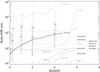 |
Fig. 9 The radio-NIR ratio as a function of redshift for different galaxy templates (solid and dashed lines). The dotted lines are the radio-NIR ratios of our sample. The radio flux density of the optically faint radio sources pertains to the total FIRST radio flux density, from the sum of the integrated power of all the FIRST components (Table 1) and the NIR emission pertains to the central NIR component, which is coincident with the center of the radio structure (components N; Table 3). The NIR magnitude system is Vega. The large dots are the median redshift values for the 3CR (dashed; Spinrad 1985) and GPS (solid; Labiano et al. 2007) sample sources, with a one σ errorbar. |
Our approach is not to rigorously derive photometric redshift estimates, but rather to assess the class of objects with which our sample galaxies are more consistent and the implied redshift range. To this end, we commence by comparing the radio-to-K- or Ks-band luminosities. Figure 9 shows the results of this exercise. The quoted NIR flux (in the Vega magnitude system) corresponds to that of the central host galaxy (components N; Table 3), which is coincident with the centers of the radio structures. The radio flux density of our optically faint radio sources is the total FIRST radio flux density (Table 7) as defined in Sect. 5.2, while for the remaining sources, the total radio flux density is the 1.4 GHz radio flux density reported in NED. The horizontal dotted lines show the measured flux ratio of the radio to NIR for our sample sources. On top of this (solid and dashed lines), we show the radio-to-NIR ratio for a range of different sources, with starburst towards the bottom and luminous radio galaxies towards the top. The large dots with error bars show the average and 68% spread around the mean for the 3CR (dashed) and GPS (solid) samples.
Figure 9 clearly shows that the majority of our sample sources possess smaller radio-to-NIR ratios than the 3CR sample, but ones that are much larger than those of starbursts, except perhaps at extremely high redshifts. However, the latter scenario is ruled out because it would lead to unrealistically high luminosities in both the radio and optical regime. Viewed as a class, the characteristics of our sample of sources are more consistent with those of GPS sources at z < 4. We stress that the heterogeneity of the GPS sample does not alter significantly the results presented in Fig. 9. Whether we use only the QSOs (z > 1) or the entire GPS sample, the result is robust; the median ratio in each redshift bin of the GPS sample will always fall below the 3CR sample.
For each template SED that the horizontal dotted lines of our sources intersect, we can obtain a redshift estimate for our sample sources. We do this by first selecting those template SEDs/redshifts that reproduce the infrared-radio slope to within 10% (approximately consistent with the error estimates). However, it is obvious from Fig. 9 that using the radio-to-NIR ratio alone does not provide a unique redshift. We therefore reject any template SED/redshift solution that would predict optical fluxes (SDSS or Stripe 82) brighter than the 1σ upper limits.
The heterogeneity of the SEDs and the limited observational data does, however, complicate our attempts to estimate rigorous redshifts for our sample sources. We do note that Mrk 668 traces fairly closely the mean trend of the GPS sources (Fig. 9). We therefore adopted this SED template in order to obtain representative redshifts for our sample sources. This might be misleading for individual targets but it is a reasonable approach given that our sample do seem to show typical infrared-radio slope values consistent with the mean GPS sample. The estimated redshifts obtained through this procedure are included in Table 7. We stress that using a template GPS source such as Mrk 668 provides only an illustrative estimate of the redshift; there is indeed a degeneracy in the redshift determination. The most robust result is that the very lowest redshift solutions are excluded when we include the optical upper limits.
We can obtain an independent check of our redshift estimates by exploiting that three of the NIR sources (components N corresponding to maxBCG 3131, 6167, and 8485) appear to have faint counterparts in the Stripe 82 images. By combining the u, g, r, i, and z (AB magnitude system) photometry from Stripe 82 with our NIR photometry, we have estimated photometric redshifts using version 2.2 of the Le Phare5 photometric redshift code (Arnouts et al. 1999; Ilbert et al. 2006). The resulting redshift estimates are included in Table 7. As can be seen, these are in very good agreement with the estimates obtained using Mrk 668 as a template. If we compare these radio source redshift estimates (Table 7) with those of the clusters and respective BCGs (Table 2), we can conclude that, although originally identified in the field-of-view of the clusters, the optically faint radio sources in our sample are not members of the SDSS clusters listed in Table 2.
An alternative interpretation of the nature of the optically faint radio sources is that they are predominantly steep spectrum radio sources, where the steep spectrum emission of the lobes dominates the radio flux. This would fit most observational results but the main obstacle lies in the radio-to-NIR ratio. While there are a few steep spectrum radio sources such as 3C 305 (Fig. 9) that have radio-to-NIR ratios lower or comparable to our sources, most have considerably higher ratios. More generally, double-lobed radio quasars from the Hough & Readhead (1989) sample lie, on average, well above our sample in the radio-NIR diagram. Even if we use 3C 305 as a template, this results in a large discrepancy between the redshift inferred from the radio-to-NIR ratio (z > 3) and that obtained from the Le Phare photometric redshift estimate (Table 7).
The result is that we have large-scale, relatively powerful radio sources similar in radio properties to 3CRR sources, but whose optical-radio slopes are consistent with those found in GPS sources. The GPS sources are compact ( ≤ 1 kpc), powerful (log P1.4 GHz ≥ 25 W Hz-1) radio sources with a well-defined peak (~1 GHz) in their radio spectra (O’Dea 1998). The spectra is generally interpreted as being produced by a contained or young radio source (O’Dea 1998).
The seemingly contradicting evidence can be reconciled by considering the so-called “double-double” radio galaxy scenario (Schoenmakers et al. 2000a; see also Stanghellini et al. 2005; Saikia & Jamrozy 2009). It is well-known that AGN have duty cycles (~109−10 years), with periods of activity (~107 years) and periods of dormancy (Saikia & Jamrozy 2009). Large-scale radio lobes are produced when the AGN jets deposit energy into intergalactic medium (IGM) “cocoons”. If the nuclear activity is halted, the luminosity of the radio lobes drops and the radio spectrum becomes steeper owing to radiation and expansion losses. However, these lobe structures are long-lived, fading away on timescales of about 107 years (Komissarov & Gubanov 1994), comparable to the timescale of the nuclear activity itself. The re-ignition of the jet-forming activity can occur via internal instability of the accretion disc (Natarajan & Pringle 1998) or gas accretion through an interaction or merger (Barnes & Hernquist 1996), potentially producing a GPS spectrum typical of a young radio source. If the AGN restart occurs within a few 107 years, the large-scale radio lobes will still be visible.
The above theory predicts a large number of such “double-double” radio sources – 3C 219 (Clarke & Burns 1991; Clarke et al. 1992), 4C 26.35 (Owen & Ledlow 1997), 3C 445 (Kronberg et al. 1986; Leahy et al. 1997), 1245+676 (Marecki et al. 2003; Bondi et al. 2004), B1834+620 (Schoenmakers et al. 2000a,b), B0925+420, B1240+389, and B1450+333 (Schoenmakers et al. 2000a), and more recently Speca, a BCG belonging to the maxBCG J212.45357-03.04237 (Hota et al. 2011) are just a few examples. Some of these sources also have GPS-type spectra – e.g. B0108+388 (Baum et al. 1990), 1245+676 (Marecki et al. 2003; Antón et al. 2004; Bondi et al. 2004), and B1834+620 (Schoenmakers et al. 2000a,b). However, GPS sources with large-scale radio emission appear to be rare (Stanghellini et al. 1990, 2005).
When compared to these classical “double-double” radio sources (Schoenmaker et al. 2000a), our optically faint radio sources have, on average, similar projected FIRST LLS and total FIRST radio powers (Table 7; Figs. 7 and 8). The similarities occur also with the 3CRR sample in terms of radio morphology, radio power, and FIRST LLS (Table 7; Figs. 1–4, 7 and 8), although our sources appear, on average, fainter in the K-band (Table 3; Fig. 8). Compared to the GPS sample (Labiano et al. 2007; see also O’Dea 1998, and Stanghellini et al. 2005), our sources have, on average, larger projected FIRST LLS, lower total (FIRST) radio powers (Table 7; Figs. 7 and 8), and fainter K-band magnitudes (Table 3; Fig. 8).
The way to reconcile the GPS-type optical-radio slope with the large-scale radio structure in our sample sources is to assume the total FIRST emission as an upper limit to the radio power of the hypothetical GPS. That we do not detect significant radio core emission in the FIRST images (except for maxBCG 2596 and possibly maxBCG 3131) is not deterministic; the moderate redshift of the sources combined with the low signal-to-noise ratio of the FIRST images may mask out the presence of this radio core. In this scenario, our sources may be regarded as re-ignited AGN, and the large-scale structure as a relic of a previous cycle of black hole activity.
Thus, based on the present evidence we would argue that while interpreting the optically faint radio sources as steep spectrum radio sources would be possible in some cases, overall our sample appear to show systematically closer agreement with a “double-double” radio source scenario in the radio-to-NIR diagram (Fig. 9). To robustly distinguish between these two scenarios, we do, however, require additional observational data for our sources. Deep, high-resolution radio observations should assess the presence of small-scale radio structures, signatures of recently re-ignited AGN activity.
These results differ somewhat from those of previous studies of radio sources with compact radio morphologies that are faint in the optical or infrared (Higdon et al. 2005, 2008; Garn & Alexander 2008; Jarvis et al. 2009; Huynh et al. 2010; Norris et al. 2011; Banfield et al. 2011). Both the observed infrared-radio correlation and SED modelling results suggest that these radio sources are mainly radio-loud AGN at z > 1 with QSO- or Seyfert 2-type spectra.
6. Conclusions
We have presented new, deep near-infrared images of a small sample of optically faint radio sources found, in projection, in low redshift galaxy cluster fields. These new observations have allowed us to detect near-infrared emitting host galaxies with Ks ~ 17–20 mag, ~1.5 arcsec in size, coincident with the centers of the radio structures.
We have constructed and analysed the SEDs of the sources by comparing them with templates of a large range of galaxy types. Considering the overall radio properties in isolation, our sources are rather similar to 3CRR sources. However, when comparing our NIR fluxes to the radio flux density, we find that our NIR fluxes are relatively too bright to be consistent with the properties of classical 3CR sources; they have instead radio-to-optical ratios similar to those found in GPS sources. The photometric redshifts estimated from the radio and NIR data assuming a GPS-like source (Mrk 668) are in good agreement with optical-NIR photometric redshift estimates, when available.
To reconcile these two observations, we suggest that our sample of optically faint radio sources have properties that are consistent with reborn AGN that retain, in their large-scale radio structure, signatures of past black hole activity. If this can be confirmed, it offers an interesting approach to study the duty-cycles and re-ignition of radio sources.
This scenario could in the future be tested by obtaining deep, high-resolution radio observations of our sources. Our proposed scheme would predict the existence of compact central sources similar to GPS sources. It would also be necessary to obtain deeper photometric and spectroscopic data to study the stellar populations of the sources and improve the accuracy of their redshift estimates.
Acknowledgments
M. E. Filho acknowledges support from the Fundação para a Ciência e Tecnologia (FCT), Ministério da Ciência e Ensino Superior, Portugal through the grant SFRH/BPD/36141/2007. S. Antón acknowledges FCT through the contract Ciência2007. All authors acknowledge support from the FCT through the grant PTDC/CTE-AST/66147/2006 for the project “Understanding Massive Galaxies in the Universe”. We would like to thank the anonymous referee for his useful suggestions. This research has made use of NED (NASA/IPAC Extragalactic Database), which is operated by the Jet Propulsion Laboratory, California Institute of Technology, under contract with the National Aeronautics and Space Administration. Funding for the SDSS and SDSS-II has been provided by the Alfred P. Sloan Foundation, the Participating Institutions, the National Science Foundation, the US Department of Energy, the National Aeronautics and Space Administration, the Japanese Monbukagakusho, the Max Planck Society, and the Higher Education Funding Council for England. The SDSS Web Site is http://www.sdss.org/. The SDSS is managed by the Astrophysical Research Consortium for the Participating Institutions. The Participating Institutions are the American Museum of Natural History, Astrophysical Institute Potsdam, University of Basel, University of Cambridge, Case Western Reserve University, University of Chicago, Drexel University, Fermilab, the Institute for Advanced Study, the Japan Participation Group, Johns Hopkins University, the Joint Institute for Nuclear Astrophysics, the Kavli Institute for Particle Astrophysics and Cosmology, the Korean Scientist Group, the Chinese Academy of Sciences (LAMOST), Los Alamos National Laboratory, the Max-Planck-Institute for Astronomy (MPIA), the Max-Planck-Institute for Astrophysics (MPA), New Mexico State University, Ohio State University, University of Pittsburgh, University of Portsmouth, Princeton University, the United States Naval Observatory and the University of Washington.
References
- Abazajian, K. N., Adelman-McCarthy, J. K., Agüeros, M. A., et al. 2009, ApJS, 182, 543 [NASA ADS] [CrossRef] [Google Scholar]
- Antón, S., Browne, I. W. A., Marchã, M. J. M., Bondi, M., & Polatidis, A. 2004, MNRAS, 352, 673 [NASA ADS] [CrossRef] [Google Scholar]
- Appleton, P. N., Fadda, D. T., Marleau, F. R., et al. 2004, ApJS, 154, 147 [NASA ADS] [CrossRef] [Google Scholar]
- Arnouts, S., Cristiani, S., Moscardini, L., et al. 1999, MNRAS, 310, 540 [NASA ADS] [CrossRef] [Google Scholar]
- Baldi, R. D., Chiaberge, M., Capetti, A., et al. 2010, ApJ, 725, 2426 [NASA ADS] [CrossRef] [Google Scholar]
- Banfield, J. K., George, S. J., Taylor, A. R., et al. 2011, ApJ, 733, 69 [NASA ADS] [CrossRef] [Google Scholar]
- Barnes, J. E., & Hernquist, L. 1996, ApJ, 471, 115 [NASA ADS] [CrossRef] [Google Scholar]
- Baum, S. A., O’Dea, C. P., Murphy, D. W., & de Bruyn, A. G. 1990, A&A, 232, 19 [NASA ADS] [Google Scholar]
- Bondi, M., Marchã, M. J. M., Polatidis, A., et al. 2004, MNRAS, 352, 112 [NASA ADS] [CrossRef] [Google Scholar]
- Clarke, D. A., & Burns, J. O. 1991, ApJ, 369, 308 [NASA ADS] [CrossRef] [Google Scholar]
- Clarke, D. A., Bridle, A. H., Burns, J. O., Perley, R. A., & Norman, M. L. 1992, ApJ, 385, 173 [NASA ADS] [CrossRef] [Google Scholar]
- Fomalont, E. B., Kellermann, K. I., Partridge, R. B., Windhorst, R. A., & Richards, E. A. 2002, AJ, 123, 240 [Google Scholar]
- Fanaroff, B. L., & Riley, J. M. 1974, MNRAS, 167, 31 [NASA ADS] [CrossRef] [Google Scholar]
- Fukugita, M., Shimasaku, K., & Ichikawa, T. 1995, PASP, 107, 945 [NASA ADS] [CrossRef] [Google Scholar]
- Garn, T., & Alexander, P. 2008, MNRAS, 391, 1000 [NASA ADS] [CrossRef] [Google Scholar]
- Haarsma, D. B., Partridge, R. B., Windhorst, R. A., & Richards, E. A. 2000, ApJ, 544, 641 [NASA ADS] [CrossRef] [Google Scholar]
- Higdon, J. L., Higdon, S. J. U., Higdon, S. J. U., et al. 2005, ApJ, 626, 58 [NASA ADS] [CrossRef] [Google Scholar]
- Higdon, J. L., Higdon, S. J. U., Willner, S. P., et al. 2008, ApJ, 688, 885 [NASA ADS] [CrossRef] [Google Scholar]
- Hopkins, A. M., Afonso, J., Chan, B., et al. 2003, AJ, 125, 465 [NASA ADS] [CrossRef] [Google Scholar]
- Hota, A., Sirothia, S. K., Ohyama, Y., et al. 2011, MNRAS, 417, L36 [NASA ADS] [CrossRef] [Google Scholar]
- Hough, D. H., & Readhead, A. C. S. 1989, AJ, 98, 1208 [NASA ADS] [CrossRef] [Google Scholar]
- Huynh, M. T., Norris, R. P., Siana, B., & Middelberg, E. 2010, ApJ, 710, 698 [NASA ADS] [CrossRef] [Google Scholar]
- Ilbert, O., Arnouts, S., McCracken, H. J., et al. 2006, A&A, 457, 841 [NASA ADS] [CrossRef] [EDP Sciences] [Google Scholar]
- Jarvis, J. M., Teimourian, H., Simpson, C., et al. 2009, MNRAS, 398, L83 [NASA ADS] [CrossRef] [Google Scholar]
- Koester, B. P., McKay, T. A., Annis, J., et al. 2007, ApJ, 660, 239 [NASA ADS] [CrossRef] [Google Scholar]
- Komissarov, S. S., & Gubanov, A. G. 1994, A&A, 285, 27 [NASA ADS] [Google Scholar]
- Kronberg, P. P., Wielebinski, R., & Graham, D. A. 1986, A&A, 169, 63 [NASA ADS] [Google Scholar]
- Labiano, A., Barthel, P. D., O’Dea, C. P., et al. 2007, A&A, 463, 97 [NASA ADS] [CrossRef] [EDP Sciences] [Google Scholar]
- Larson, D., Dunkley, J., Hinshaw, G., et al. 2011, ApJS, 192, 16 [NASA ADS] [CrossRef] [Google Scholar]
- Leahy, J. P., Black, A. R. S., Dennett-Thorpe, J., et al. 1997, MNRAS, 291, 20 [NASA ADS] [Google Scholar]
- Ledlow, M. J., & Owen, F. N. 1996, AJ, 112, 9 [NASA ADS] [CrossRef] [Google Scholar]
- Machalski, J., Jamrozy, M., & Zola, S. 2001, A&A, 371, 445 [NASA ADS] [CrossRef] [EDP Sciences] [Google Scholar]
- Marecki, A., Barthel, P. D., Polatidis, A., & Owsianik, I. 2003, PASA, 20, 16 [NASA ADS] [CrossRef] [Google Scholar]
- Middelberg, E., Norris, R. P., Cornwell, T. J., et al. 2008a, AJ, 135, 1276 [NASA ADS] [CrossRef] [Google Scholar]
- Natarajan, P., & Pringle, J. E. 1998, ApJ, 506, 97 [Google Scholar]
- Norris, R. P., Afonso, J., Appleton, P. N., et al. 2006, AJ, 132, 2409 [NASA ADS] [CrossRef] [Google Scholar]
- Norris, R. P., Afonso, J., Cava, A., et al. 2011, ApJ, 736, 55 [NASA ADS] [CrossRef] [Google Scholar]
- O’Dea, C. 1998, PASP, 110, 4930 [Google Scholar]
- O’Dea, C. P., & Baum, S. A. 1997, AJ, 113, 148 [NASA ADS] [CrossRef] [Google Scholar]
- Owen, F. N., & Ledlow, M. J. 1997, ApJS, 108, 41 [NASA ADS] [CrossRef] [Google Scholar]
- Richards, E. A. 1999, ApJ, 513, 9 [Google Scholar]
- Richards, G. T., Fan, X., Schneider, D. P., et al. 2001, AJ, 121, 2308 [NASA ADS] [CrossRef] [Google Scholar]
- Rigby, E. E., Snellen, I. A. G., & Best, P. N. 2007, MNRAS, 380, 1449 [NASA ADS] [CrossRef] [Google Scholar]
- Saikia, D. J., & Jamrozy, M. 2009, BASI, 37, 63 [Google Scholar]
- Schoenmakers, A. P., de Bruyn, A. G., Röttgering, H. J. A., van der Laan, H., & Kaiser, C. R. 2000a, MNRAS, 315, 371 [NASA ADS] [CrossRef] [Google Scholar]
- Schoenmakers, A. P., Schoenmakers, A. P., & Röttgering, H. J. A., et al. 2000b, MNRAS, 315, 381 [Google Scholar]
- Spinrad, H., Marr, J., Aguilar, L., & Djorgovski, S. 1985, PASP, 97, 932 [NASA ADS] [CrossRef] [Google Scholar]
- Spoon, H. W. W., Graham, J. R., Akeson, R. L., et al. 2007, ApJ, 654, 77 [Google Scholar]
- Stanghellini, C., Baum, S. A., O’Dea, C. P., & Morris, G. B. 1990, A&A, 233, 379 [NASA ADS] [Google Scholar]
- Stanghellini, C., O’Dea, C. P., Dallacasa, D., et al. 2005, A&A, 443, 891 [NASA ADS] [CrossRef] [EDP Sciences] [Google Scholar]
- Sullivan, M., Hopkins, A. M., Afonso, J., et al. 2004, ApJS, 155, 1 [NASA ADS] [CrossRef] [Google Scholar]
- White, R. L., Becker, R. H., Helfand, D. J., & Gregg, M. D. 1997, ApJ, 475, 479 [NASA ADS] [CrossRef] [Google Scholar]
- York, D. G., Adelman, J., Anderson, J. E., Jr., et al. 2000, AJ, 120, 1579 [Google Scholar]
- Yun, M. S., Reddy, N. A., & Condon, J. J. 2001, ApJ, 554, 803 [NASA ADS] [CrossRef] [Google Scholar]
- Zinn, P.-C., Middelberg, E., & Ibar, E. 2011, A&A, 531, A14 [NASA ADS] [CrossRef] [EDP Sciences] [Google Scholar]
All Tables
All Figures
|
Fig. 1 From left to right, inverted greyscale image of the NIR emission, FIRST greyscale emission with superimposed radio contours, the first two levels of the FIRST contour plots superimposed on the NIR field and likewise superimposed on the SDSS and the Stripe 82 (maxBCG 3131) rAB-band field. The field numbers are the sequential numbers of SDSS macxBCG cluster fields to which the radio sources belong, as they appear in Koester et al. (2007), letters/numbers are the NIR components and lobe designations refer to the radio components. The inlays contain the NIR N component (Tables 3 and 4), coincident with the center of the radio structure. Radio contours are: (top) 0.001, 0.002, 0.004, 0.008 mJy; (bottom) 0.001, 0.002, 0.004, 0.008 mJy. |
| In the text | |
|
Fig. 2 From left to right, inverted greyscale image of the NIR emission, FIRST greyscale emission with superimposed radio contours, the first two levels of the FIRST contour plots superimposed on the NIR field and likewise superimposed on the SDSS field and the Stripe 82 (maxBCG 6167 and 8495) rAB-band field. The field numbers are the sequential numbers of SDSS macxBCG cluster fields to which the radio sources belong as they appear in Koester et al. (2007), letters/numbers are the NIR components and lobe designations refer to the radio components. The inlays contain the NIR N component (Tables 3 and 4), coincident with the center of the radio structure. Radio contours are: (top) 0.0004, 0.0008, 0.0016 mJy (in log); (bottom) 0.0005, 0.0010, 0.0020, 0.0040, 0.0060, 0.0080 mJy. |
| In the text | |
|
Fig. 3 From left to right, inverted greyscale image of the NIR emission, FIRST greyscale emission with superimposed radio contours, the first two levels of the FIRST contour plots superimposed on the NIR field and likewise superimposed on the SDSS rAB-band field. The field numbers are the sequential numbers of SDSS macxBCG cluster fields to which the radio sources belong, as they appear in Koester et al. (2007), letters/numbers are the NIR components and lobe designations refer to the radio components. The inlays contain the NIR N component (Tables 3 and 4), coincident with the center of the radio structure. Radio contours are: (top) 0.001, 0.002, 0.004, 0.008, 0.016 mJy; (bottom) 0.008, 0.0016, 0.0032, 0.0064, 0.0128, 0.0256, 0.0512 mJy. |
| In the text | |
|
Fig. 4 From left to right, inverted greyscale image of the NIR emission, FIRST greyscale emission with superimposed radio contours, the first two levels of the FIRST contour plots superimposed on the NIR field and likewise superimposed on the SDSS rAB-band field. The field numbers are the sequential numbers of SDSS macxBCG cluster fields to which the radio sources belong, as they appear in Koester et al. (2007), letters/numbers are the NIR components and lobe designations refer to the radio components. The inlays contain the NIR N component (Tables 3 and 4), coincident with the center of the radio structure. Radio contours are: (top) 0.0004, 0.0008, 0.0016, 0.0032 mJy (in log); (bottom) 0.0005, 0.0010, 0.0020, 0.0040, 0.0080 mJy. |
| In the text | |
|
Fig. 5 The NIR versus 1.4 GHz FIRST flux density. The NIR flux pertains to the Ks-band fluxes of the NIR components (components N; Table 3) coincident with the radio structure centers. The NIR magnitudes are in the Vega system. The radio core flux density (top) pertains to the radio “core” flux density (Table 6) estimated using funtools on circular regions of approximately the same size (~2 arcsec) and centered on the NIR emission regions N (Table 3; see Sect. 5.2). The total radio flux density (bottom) pertains to the total FIRST flux density as a sum of the flux density of all the FIRST components (Table 1). The errorbar associated with the FIRST flux density corresponds to 1 × rms, where rms is the root mean square, a measure of the noise level in the FIRST image. |
| In the text | |
|
Fig. 6 The redshift distribution of the 3CRR (solid line) and GPS (dashed line) sample. |
| In the text | |
|
Fig. 7 The redshift versus largest linear size (LLS) for the 3CRR (crosses), GPS (triangles), and our sample (circles). The LLS for the GPS sources were obtained from O’Dea & Baum (1997), when a measurement was available. |
| In the text | |
|
Fig. 8 Clockwise from the top left: the redshift versus the 5 GHz power for the 3CRR (crosses), GPS (triangles), and our sample total (closed circles) and core (open circles); the largest linear size (LLS) versus the 5 GHz power for the 3CRR (crosses), GPS (triangles), and our sample total (closed circles) and core (open circles); the redshift versus the K- (GPS and 3CRR) or Ks-band (our sample) magnitude for the 3CRR (crosses), GPS (triangles), and our sample (circles); the K- (GPS and 3CRR) or Ks-band (our sample) magnitude versus the 5 GHz power for the 3CRR (crosses), GPS (triangles), and our sample total (closed circles) and core (open circles). The radio measurements for the 3CRR sample are those of the radio cores, and for the GPS sample it is the total radio power. For our sample, we include the radio “core” power (open circles; Table 7) estimated using funtools in circular regions of approximately the same size (~2 arcsec) and centered on the NIR emission regions N (Table 3; see Sect. 5.2) and the total radio power (closed circles; Table 7), the sum of the power of all the FIRST components (Table 1). We assumed a flat radio spectrum for all sources in order to normalize to 5 GHz. The LLS for the GPS sample were derived from O’Dea & Baum (1997), when a measurement was available. The 3CRR K-band magnitudes are aperture- and emission-line-corrected measurements for a subset of 3CRR sources. For the GPS sample, the K-band magnitudes were obtained by interpolation from NED NIR photometric points. NIR magnitudes for our sample are for the central NIR component, coincident with the center of the radio structure (components N; Table 3). The NIR magnitude system is Vega. |
| In the text | |
|
Fig. 9 The radio-NIR ratio as a function of redshift for different galaxy templates (solid and dashed lines). The dotted lines are the radio-NIR ratios of our sample. The radio flux density of the optically faint radio sources pertains to the total FIRST radio flux density, from the sum of the integrated power of all the FIRST components (Table 1) and the NIR emission pertains to the central NIR component, which is coincident with the center of the radio structure (components N; Table 3). The NIR magnitude system is Vega. The large dots are the median redshift values for the 3CR (dashed; Spinrad 1985) and GPS (solid; Labiano et al. 2007) sample sources, with a one σ errorbar. |
| In the text | |
Current usage metrics show cumulative count of Article Views (full-text article views including HTML views, PDF and ePub downloads, according to the available data) and Abstracts Views on Vision4Press platform.
Data correspond to usage on the plateform after 2015. The current usage metrics is available 48-96 hours after online publication and is updated daily on week days.
Initial download of the metrics may take a while.