| Issue |
A&A
Volume 536, December 2011
|
|
|---|---|---|
| Article Number | A51 | |
| Number of page(s) | 8 | |
| Section | Atomic, molecular, and nuclear data | |
| DOI | https://doi.org/10.1051/0004-6361/201117348 | |
| Published online | 06 December 2011 | |
Atomic data of Zn I for the investigation of element abundances⋆
1
Department of Physics, College of ScienceNational University of Defense Technology, 410073 Changsha, Hunan, PR China
e-mail: This email address is being protected from spambots. You need JavaScript enabled to view it.
2
National Astronomical Observatories, Chinese Academy of Sciences, 100012 Beijing, PR China
Received: 26 May 2011
Accepted: 9 September 2011
Abstract
Aims. We calculate the energy levels, oscillator strengths, and photoionization cross-sections of Zn I to provide atomic data for the study of element abundances in astrophysics.
Methods. The calculations are carried out by using the R-matrix method in the LS-coupling scheme. The lowest 12 terms of Zn II are utilized as target states and extensive configuration interaction is included to properly delineate the quantum states of Zn II and Zn I.
Results. The 3443 oscillator-strength values are calculated in both length and velocity forms, for the dipole-allowed transitions between 235 bound states of Zn I. The photoionization cross-section of each bound state is presented in a photon energy range from the first threshold to about 1.5 Ry. Some resonance structures are identified in the photoionization cross-sections.
Conclusions. A set of atomic data to derive the spectral characteristics of neutral zinc is obtained. Comparisons are made with available experimental and other theoretical results.
Key words: stars: abundances / atomic data
The complete set of atomic data is only available at the CDS via anonymous ftp to cdsarc.u-strasbg.fr (130.79.128.5) or via http://cdsarc.u-strasbg.fr/viz-bin/qcat?J/A+A/536/A51
© ESO, 2011
1. Introduction
Accurate determination of the abundance of zinc is important to investigate the chemical evolution of both damped Lyα systems (Pettini et al. 1997) and our Galaxy (Allen et al. 2011; Bihain et al. 2004). Bisterzo et al. (2004) determined the Zn abundances for stars of different stellar populations and metallicities based on high resolution spectra. Using the most widely available stellar nucleosynthesis expectations, they found that the abundance of zinc is central to inferring its astrophysical origin. It has been recognized that it is important to consider the effects of non-local thermodynamic equilibrium (NLTE) when determining element abundances (Asplund 2005). Research has shown that NLTE can strongly affect the abundances of Na, Mg, Al, Si, K, and Ca (Andrievsky et al. 2007, 2008, 2010; Gehren et al. 2004, 2006; Mashonkina et al. 2008; Shi et al. 2008) and these effects are sensitive to the accuracy of the atomic data used in the NLTE modeling. An adequate atomic model requires a complete set of atomic data, and the development of such a model is a difficult task for Zn owing to its complex atomic structure (Mishenina et al. 2002). To the best of our knowledge, the only published study of the effects of NLTE of Zn abundance is Takeda et al. (2005), who used the photoionization cross-sections derived from hydrogenic approximation. There is therefore an urgent need to obtain a complete set of accurate atomic data for Zn.
Energy levels, oscillator strengths, and photoionization cross-sections are the basic atomic parameters. The energy levels of Zn I were published by Moore (1971) and comprehensively summarized by Sugar & Musgrove (1995), whereas the oscillator strengths and the photoionization cross-sections of Zn I are not widely available in the literature.
Experimental studies of the oscillator strengths of Zn I were addressed by Landman & Novick (1964) and Lurio et al. (1964), who measured the lifetime of the excited state 3d104s4p  . The lifetimes of more quantum states including 3d104s4p were measured by Martinson et al. (1979) and Zerne et al. (1994). Kerkhoff et al. (1980) measured the oscillator strengths for transitions of 3d104sns 3S–3d104smp
  and 3d104sn′d 3D–3d104smp (n = 5 − 7,n′ = 4 − 6,m = 4,5). From the theoretical point of view, Hibbert (1989) calculated the oscillator strength of the resonance transition 3d104s21S–3d104s4p using model potentials. The oscillator strength of the same transition was discussed by Brage & Froese Fischer (1992) using a multi-configuration Hartree-Fock (MCHF) approach that considered the core polarization effects. Glowacki & Migdalek (2006) and Chen & Cheng (2010) carried out relativistic configuration interaction (CI) calculations for the transition rates of 3d104s2
 –3d104s4p
  and 3d104s2–3d104s4p
  .
.
Most investigations of the photoionization of Zn I have focused on the ground state 3d104s21S. Marr & Austin (1969) and Harrison et al. (1969) measured the photoionization cross-section of Zn I in the photon energy range of 0.69–1.22 and 0.73–3.69 Ry, respectively. The d-shell absorption spectrum was presented and analyzed by Sommer et al. (1987) using synchrotron radiation as the background source. Photoionization cross-sections for the 4s, 3d, 3p, 3s subshells of Zn I were calculated by Fliflet & Kelly (1974, 1976) using many-body perturbation theory. Bartschat (1987) calculated the photoionization cross-section of the ground state 3d104s21S for Zn I by using the semirelativistic R-matrix method based on the Breit-Pauli Hamiltonian, while Stener & Decleva (1997) presented time-dependent local density approximation (TDLDA) calculations for the photoionization of the ground state. Froese Fischer & Zatsarinny (2007) calculated the photoionization of the 4s4p excited states using the MCHF approach and the B-spline R-matrix method.
The atomic data presented above, either experimental or theoretical, are insufficient for building a practical NLTE model for the investigation of the Zn abundance, as such a model would need a complete and consistent set of atomic data involving a large number of quantum states. In this work, we aim to provide a complete set of atomic data including the energy levels, oscillator strengths, and photoionization cross-sections for Zn I. The present calculations are carried out using the R-matrix program1, which is a modified version of the Belfast atomic R-matrix program RMATRX1 (Berrington et al. 1995). Extensive CI is taken into account to ensure that accurate atomic data can be obtained.
2. Theoretical methods
The R-matrix method is a kind of close-coupling approach to the analysis of electron-atom and photon-atom interactions, which was described in great detail by Burke et al. (1971) and Berrington et al. (1987). The outline of this method is briefly presented in the following, where LS-coupling is assumed. In the internal region, the wave functions of the (N + 1)-electron system are depicted as linear combinations of the energy-independent basis states ψk that are expanded in the form 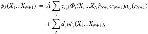 (1)where  is the antisymmetrization operator that takes the exchange effects between the target electrons and the (N + 1)th electron into account, and i is the channel symbol. The term Xm stands for the spatial (rm) and the spin (σm) coordinates of the mth electron. The Φi are channel functions consisting of CI wavefunctions for the residual ion coupled with spin-angle functions for the (N + 1)th electron to give an eigenstate of definite total orbital angular momentum L and total spin S. The functions uij(r) in the first term on the right hand side of Eq. (1), which are normally obtained from appropriate equations and boundary conditions, form the basis sets for the continuum wavefunctions of the (N + 1)th electron. The {φj} in the second term on the right hand side of Eq. (1) are (N + 1)-electron bound states that are eigenstates with the same L and S, and they are included to allow for electron correlation effects. In the external region, the exchange effects between the target electrons and the (N + 1)th electron have been ignored and the radial functions Fi(r) of the (N + 1)th electron can be obtained by directly integrating the radial equations. Matching the two regions at the R-matrix radius provides a scattering matrix and the wave functions of the (N + 1)-electron system, hence the dipole transition probabilities.
The one-electron orbitals of bound states from which the {φj} are constructed are represented as linear combinations of Slater-type orbitals 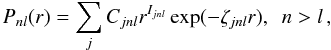 (2)where the parameters Cjnl and ζjnl are determined variationally by optimizing the energies of specific LS-coupled states. In practice, the Slater-type coefficients Cjnl are replaced by Clementi-type coefficients Gjnl as
 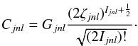 (3)
(3)
In this work, we employed 12 orbitals of Zn II. The orbitals 1s, 2s, 2p, 3s, 3p, 3d, 4s were chosen to be HF functions given by Clementi & Roetti (1974) for the ground state 3d104s 2S of Zn II. However, 3d and 4s were adjusted by minimizing a linear combination of the ground state and 3d94s22D with the CIV3 computer code (Hibbert 1975). The orbitals 4p, 4d, 5s, 5p were obtained by optimizing linear combinations of the energies of the corresponding 3d10nl (occupying a weight of 99.6%) and 3d94sn′l′ (the same LS term as 3d10nl occupying a weight of 0.4%) states, respectively. The only pseudo orbital  was obtained by optimizing the state of 3d94s22D. The relevant parameters of the valence orbital radial functions are listed in Table 1.
Orbital parameters of the radial functions obtained with the CIV3 code for Zn II.
The R-matrix radius was chosen to be 36.0 a.u. to ensure that the wavefunctions of bound states were completely wrapped within the R-matrix sphere. As for the construction of the continuum states, the number of the continuum basis functions uij(r) was set to be 75. The 12 lowest terms of Zn II were utilized as target states, whose energy levels are listed in Table 2.
Energy levels (in Ry) for the target states of Zn II in different scales of configuration interaction.
To adequately describe the target states, extensive CI was included in the present work. To show the CI effects on the energy levels of the target states, we present three sets of calculations in Table 2, which are represented by cases A, B, and C, respectively. In case A, a single electron excitation is allowed from 3d and 4s subshells of the ground configuration 3d104s excluding subshell. Explicitly, configurations of 3d104s, 3d104p, 3d104d, 3d105s, 3d105p, 3d94s2, 3d94s4p, 3d94s4d, 3d94s5s, and 3d94s5p were included in the calculation. In case B, in addition to configurations included in case A, two electron excitations are allowed from 3d and 4s subshells of the configuration 3d94s2, excluding subshell. Therefore, in addition to configurations included in case A, the following configurations were taken into account: 3d94p2, 3d94p4d, 3d94p5s, 3d94p5p, 3d94d2, 3d94d5s, 3d94d5p, 3d95s2, 3d95s5p, 3d95p2, 3d84s24p, 3d84s24d, 3d84s25s, 3d84s25p, 3d84s4p2, 3d84s4p4d, 3d84s4p5s, 3d84s4p5p, 3d84s4d2, 3d84s4d5s, 3d84s4d5p, 3d84s5s2, 3d84s5s5p, 3d84s5p2, 3d74s24p2, 3d74s24p4d, 3d74s24p5s, 3d74s24p5p, 3d74s24d2, 3d74s24d5s, 3d74s24d5p, 3d74s25s2, 3d74s25s5p, and 3d74s25p2. In case C, two electron excitations are allowed from either the 3d or 4s subshells of the configuration 3d94s2, including excitations to the subshell, and five additional configurations are included to describe the target states. In addition to the configurations included in cases A and B, the following configurations were included in case C: 3d105d, 3d94s5d, 3d94p5d, 3d94d5d, 3d95s5d, 3d95p5d, 3d95d2, 3d84s25d, 3d84s4p5d, 3d84s4d5d, 3d84s5s5d, 3d84s5p5d, 3d84s5d2, 3d84p25d, 3d84p4d5d, 3d84p5s5d, 3d84p5p5d, 3d84p5d2, 3d74s24p5d, 3d74s24d5d, 3d74s25s5d, 3d74s25p5d, and 3d74s25d2.
In Table 2, we also give the experimental energy levels compiled by Sugar & Musgrove (1995). One can find that the energies of the target states become closer and closer to the experimental results as the CI scale increases from case A to C. In the following, all results on the energy levels, oscillator strengths, and photoionization cross-sections were obtained by using the CI in case C.
3. Results and discussions
Using the method described above, we calculated the energy levels of the bound states, bound-bound oscillator strengths, and photoionization cross-sections of Zn I.
3.1. Bound states of Zn I
We obtained 235 bound states of different symmetries (characterized by total orbital angular momentum and spin and parity) in this work. The energy levels of some of the lowest bound states and several high Rydberg states are listed in Table 3, together with the experimental data (Sugar & Musgrove 1995). From the inspection of Table 2, one can see that the calculated energies of the target states are a little lower than the experimental results, except for the term of 3d94s22D. This shows that the energy of the ground term 3d104s 2S was slightly overestimated in the calculation. Such an overestimate is due to the complexity of atomic structure of Zn. To better describe 3d104s 2S and 3d94s22D, one has to include electron correlations with three and four electron excitations from orbital 3d and higher orbitals, such as that of n = 6. Nevertheless such a larger scale of CI is untractable. In addition, relativistic effects may play a role in describing atomic structure. As a result, the energy of the ground term 3d104s21S of Zn I was overestimated. The calculated ionization energy of Zn I is 0.66614 Ry. To make a more helpful comparison with the experiment, we set the energy of the ground term 3d104s21S of Zn I to 0.02432 Ry in Table 3, which is the difference between the calculated and experimental value (0.69046 Ry). In this way, most of the calculated energy levels are in closer agreement with the experimental data.
Energy levels (in Ry) of bound states for Zn I.
Several high Rydberg states given in Table 3 show the correct order of energy even at the principal quantum numbers n = 18, 19, and 20. For the states with high principal quantum number n, the energies tend to be degenerate. For example, the energies of 3d104s8g 3G (0.67481 Ry), 3d104s8h 3H° (0.67483 Ry), and 3d104s8i 3I (0.67484 Ry) are very close and nearly degenerate. Such a conclusion is consistent with the basic theory of atomic structure and spectra (Cowan 1981). The treatment of this degeneracy of Rydberg states is a great challenge of the theory. One must be very careful to assign the correct state order in the calculations. The energies of a Rydberg series become closer to the experimental values as the principal quantum number n increases, which can be found from 3d104snp 1P° and 3d104snd 1D (n = 8,10,14,18 − 20) of the Rydberg series. This indicates that our method is effective for high Rydberg states.
3.2. Oscillator strengths
For the zinc atom, the observed lines are mainly concentrated into bound-bound transitions between configurations of the Rydberg series 3d104snl (n = 4 − 7, l = 0,1,2) (Ralchenko et al. 2010). In Table 4, we compare our calculated weighted oscillator strengths (gf-values) for some dipole allowed transitions with experimental and other theoretical results in the literature. The on-line data provided by Kurucz2 are also listed, which were mostly derived from the theoretical work of Warner (1968), in only a few of cases from experiments. Experimental values are given between the fine-structure levels instead of LS-coupled terms, hence we give the gf-values according to LS terms wherever possible. The symbol “*” denotes that the experimental data do not contain any contribution to the final states of Jf = 1, as a result the experimental data are smaller in value than our theoretical results. Most gf-values in length form in Table 4 have a relative difference of smaller than 20% with experimental data. For the transition of 4s4p 1P°–4s6s 1S, the relative difference between gf-values in length form of this work and that of Warner is 50%. For this transition, the oscillator strength is very small and thus sensitive to the wavefunctions and CI included in the calculation. Warner carried out his calculation based on the scaled Thomas-Fermi-Dirac (STFD) wavefunctions, which differs from those adopted in the present work.
As an illustrative example, we give the weighted oscillator strengths of transitions between the Rydberg series of 3d104snd 3D and 3d104sn′f  of Zn I in Table 5. Some gf-values in Table 5 are negative, because the initial and final terms are reversed. Taking transition series 4s4d − 4snf, 4s5d − 4smf, 4s4f − 4snd and 4s5f − 4smd (n = 4 − 12, m = 5 − 12) as examples, one can find that as the principal quantum number n increases, the oscillator strengths of a Rydberg series generally decrease quite fast. This can be understood qualitatively from the general trends of oscillator strengths (Cowan 1981). For a Rydberg series of transition, among other factors such as transition energies and angular momentum, the oscillator strengths and the effective quantum numbers n∗ have the approximate relation
 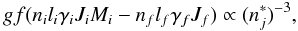 (4)and this relation stands reasonably for higher principal quantum number nj.
From the inspection of Tables 4 and 5, generally good agreements are found between the length and velocity forms of our oscillator strengths. In Table 5, the relative differences between the length and velocity forms are smaller than 7%. In Table 4, such a relative difference is smaller than 30% (majority of which are smaller than 10%) except for transitions of 1S–. For the transitions of 4s2 1S–4s4p 1P° and 4s4p 1P°–4s5s 1S, the length form of oscillator strengths agree better with the experiments, hence the length form is more reliable. To evaluate the quality of the calculated oscillator strengths as a whole, we show the velocity form versus the length form of absolute gf-values in Fig. 1 for the bound-bound transitions whose absolute gf-values are greater than 0.001 in all of the 3443 dipole-allowed transitions. Since the data cover five orders of magnitude, we adopted the logarithm coordinates for both the length and velocity forms. For thousands of calculated gf-values, nearly all of them are centered at the line corresponding to equality between the two forms, especially for larger gf-values. Such a generally good agreement between the velocity and length forms of the oscillator strengths is an indication of quality for the present calculation, although scope remains for some improvement in the accuracy of the results.
gf-values compared with experimental data and other theoretical results for Zn I.
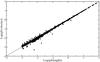 |
Fig. 1 Velocity vs. length forms for the oscillator strengths of Zn I. |
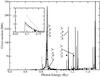 |
Fig. 2 Photoionization cross-section for the ground state 3d104s2 1S of Zn I. The solid line represents the cross-section in the present work. The dotted line represents the theoretical result carried out by Bartschat (1987). The dashed line and the filled circles represent the experimental data from Marr & Austin (1969) and Harrison (1969), respectively. The inset at the top left corner is the cross-section near threshold shown on an expanded scale. |
gf-values for the transition series 3d104snd 3D–3d104sn′f 3F° of Zn I.
3.3. Photoionization cross-sections
In stellar atmospheres, photoionization of neutral species are crucial because they are photoionization-dominated atoms (Asplund 2005). Photoionization cross-sections are much more important for the ground and several lowest excited states. In the following, we present in detail the photoionization cross-sections of the ground state 3d104s2 1S, the first excited state 3d104s4p 3P°, the second excited state 3d104s4p 1P°, and the third excited state 3d104s5s 3S for Zn I, although the photoionization cross-sections of all bound states were performed in a photon energy range from the first threshold to about 1.5 Ry in this work. Furthermore, the Rydberg series of 3d104sns (n = 5 − 8) 3S are presented to show the general trend of a Rydberg series.
Figure 2 shows the photoionization cross-section for
the ground state of Zn I in a solid line. To compare with the experimental results, we
show the experimental data from Marr & Austin (1969) and Harrison et al. (1969) as a
dashed line and filled circles, respectively. The cross-section near the threshold is
shown on an expanded scale at the top left corner, and is shifted by 0.02432 Ry, which is
the difference between the calculated ionization potential of the ground state and the
experimental value shown in Table 3. In the energy
range of the 3d94s24p resonance, Marr & Austin’s experiment
exhibited three resonance peaks, a weak resonance at about 0.82 Ry of the photon energy
and the double maximum near 0.87 Ry. The authors labeled the weak resonance at 0.82 Ry as  , and the double maximum as resonances
  and
and  . Nevertheless, there is clearly inconsistency among the
energy levels of Zn I (Sugar & Musgrove 1995),
because the energy levels of , , and are 0.82221, 0.86761, and 0.87292 Ry, respectively.
Moreover, the transition probability of the dipole allowed transition
. Nevertheless, there is clearly inconsistency among the
energy levels of Zn I (Sugar & Musgrove 1995),
because the energy levels of , , and are 0.82221, 0.86761, and 0.87292 Ry, respectively.
Moreover, the transition probability of the dipole allowed transition  should be stronger than the dipole forbidden
transitions
should be stronger than the dipole forbidden
transitions  and
and  . Fortunately, Bartschat (1987) analyzed these resonances with a semirelativistic R-matrix method, which
enabled them to classify the weak resonance at 0.82 Ry as , and to establish that the double maximum near 0.87 Ry
originated from the interference of the strong resonance with the weak resonance that in turn produced a minimum located in
the center of the strong resonance peak. The photoionization cross-section
obtained by Bartschat is indicated by a dotted line in Fig. 2. The resonances of
. Fortunately, Bartschat (1987) analyzed these resonances with a semirelativistic R-matrix method, which
enabled them to classify the weak resonance at 0.82 Ry as , and to establish that the double maximum near 0.87 Ry
originated from the interference of the strong resonance with the weak resonance that in turn produced a minimum located in
the center of the strong resonance peak. The photoionization cross-section
obtained by Bartschat is indicated by a dotted line in Fig. 2. The resonances of  ,
,  , and
, and  are not shown as the maximal cross-sections of these
resonances were unknown from Fig. 1 given by
Bartschat. Since the LS-coupling scheme is used in this work, the present approach cannot
reproduce the spin forbidden transitions from the ground term
3d104s2 1S to
3d94s24p 3P° and
3d94s24p 3D° autoionization states.
are not shown as the maximal cross-sections of these
resonances were unknown from Fig. 1 given by
Bartschat. Since the LS-coupling scheme is used in this work, the present approach cannot
reproduce the spin forbidden transitions from the ground term
3d104s2 1S to
3d94s24p 3P° and
3d94s24p 3D° autoionization states.
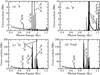 |
Fig. 3 Photoionization cross-sections for the first excited state 3d104s4p 3P° of Zn I. The partial wave cross-sections of 3S, 3P and 3D are displayed in a), b), and c), respectively, and the total cross-section is displayed in d). The solid lines represent the length forms of cross-sections, and the dashed lines represent velocity forms. |
For the photoionization of the first excited state 3d104s4p 3P° of Zn I, there are three allowed final channels 3S, 3P and 3D according to the dipole selection rule. The partial waves 3S and 3D contain a contribution from the first ionization threshold 0.40268 Ry, while the energetically lowest ionization channel of partial wave 3P opens from the second ionization threshold 3d104p 2P° (0.84082 Ry). Figure 3 shows these partial-wave cross-sections and the total cross-section of 3d104s4p 3P°, where the partial-wave cross-sections of 3S, 3P, and 3D are displayed in the sub-pictures (a), (b), and (c) respectively, and the total cross-section is displayed in (d). Solid lines in Fig. 3 represent the length forms of the cross-sections, while dashed lines represent the velocity form, and the two forms closely agree with each other. It can be seen that the 3P partial cross-section clearly contains a contribution from the photon energy of 0.9 Ry. In Figs. 3a and 3c, the first autoionization resonances of partial waves 3S and 3D are produced by the configuration 3d104p5p, not by the configuration 3d104p2, because two equivalent electrons in the 4p subshell cannot form the triplet symmetries 3D and 3S according to the Pauli exclusion principle. Figure 3c also shows a broad and strong resonance, which should be caused by 3d94s4p2 3D, whose positions are in the energy range of the resonances 3d94s2nd 3D (n = 4,5). These resonances of the partial 3D are much stronger than any other partial symmetries 3S and 3P in the shown photon energy range.
Figures 4a and 4b show the partial photoionization cross-sections of 1S and 1D for the second excited state 3d104s4p 1P° of Zn I. As the first excited triplet state 3d104s4p 3P°, the 1S and 1D partial-wave photoionization cross-sections for the second excited state contain a contribution from the first ionization threshold 0.25705 Ry, while the energetically lowest ionization channel of the partial wave 1P opens from the second ionization threshold 3d104p 2P° (0.69519 Ry) and its partial cross-section is lower than 0.01 Mb until the photon energy exceeds 0.86 Ry. Therefore, we did not give the partial cross-section of 1P symmetry. Solid and dashed lines represent the length and velocity forms of photoionization cross-sections, respectively. It is quite clear that the first resonances of 1D and 1S partial waves for the photoionization cross-sections of 3d104s4p 1P° are both produced by the configuration 3d104p2.
From the inspection of Fig. 4, it can be seen that the autoionization resonances of 3d104p2 1S and 1D have completely different characteristics. The former is narrow with an autoionization width being about 0.004 Ry and the peak cross-section of nearly 300 Mb, while the latter is a giant resonance with a width exceeding 0.1 Ry. To distinguish more clearly the resonance of 3d104p2 1S, the cross-section near the resonance are redrawn in the inset of Fig. 4a on a logarithmic scale. These two resonances were carefully investigated by Froese Fischer & Zatsarinny (2007) using both the MCHF and B-spine R-matrix methods and their results are shown in Fig. 4 in dotted lines. To enable a clearer comparison, their results have been shifted by 0.007 Ry toward lower photon energy. One can see that there is generally good agreement between our own and their results near the two resonances.
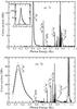 |
Fig. 4 1S and 1D partial photoionization cross-sections of 3d104s4p 1P° for Zn I. Solid and dashed lines represent the length and velocity forms of cross-sections, and the dotted lines represent the theoretical results carried out by Froese Fischer & Zatsarinny (2007). The inset in a) is the cross-section near the resonance of 3d104p2 1S on a logarithmic scale. |
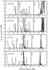 |
Fig. 5 Photoionization cross-sections of the Rydberg series 3d104sns 3S (n = 5–8 from the top down). |
Photoionization cross-sections of the Rydberg series
3d104sns 3S (n = 5, 6, 7, and
8) are displayed in Fig. 5. One can see that with the
increase in the principal quantum number n, the ionization potential
decreases, and the cross-section in the threshold increases, but it falls off fast as
photon energy increases near the threshold. This is consistent with the basic theory of
atomic structure (Cowan 1981). For photoionization
of the Rydberg state with a high principal quantum number n, the
cross-section near the threshold tends to be hydrogenic according to 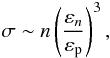 (5)where εn is
the threshold ionization energy for the shell n, and
εp is the photon energy. In addition, the peak value of the
same resonance decreases from the top down for 3d94s24p,
3d104p5s, and 3d94s25p autoionization states, yet for higher
n autoionized states such as 3d104pns and
3d104pnd , the strongest photoionization cross-section occurs for
the respective state of 3d104sns 3S, where the
principal quantum number n is identical to that of the autoionized
states. This conclusion is similar to the bound-bound transitions, as shown in Table 5, which considers the transitions of
3d104snd 3D–3d104sn′f 3F°
of Zn I as an example to illustrate such characteristics. For transitions from the state
of 4s4d 3D, the value of the oscillator strengths decreases with increasing
Rydberg series of 3d104sn′f 3F°, while for
transitions from the initial state of 4s5d 3D, the maximal oscillator strengths
occurs for 3d104s5f 3F°, not for
3d104s4f 3F°.
(5)where εn is
the threshold ionization energy for the shell n, and
εp is the photon energy. In addition, the peak value of the
same resonance decreases from the top down for 3d94s24p,
3d104p5s, and 3d94s25p autoionization states, yet for higher
n autoionized states such as 3d104pns and
3d104pnd , the strongest photoionization cross-section occurs for
the respective state of 3d104sns 3S, where the
principal quantum number n is identical to that of the autoionized
states. This conclusion is similar to the bound-bound transitions, as shown in Table 5, which considers the transitions of
3d104snd 3D–3d104sn′f 3F°
of Zn I as an example to illustrate such characteristics. For transitions from the state
of 4s4d 3D, the value of the oscillator strengths decreases with increasing
Rydberg series of 3d104sn′f 3F°, while for
transitions from the initial state of 4s5d 3D, the maximal oscillator strengths
occurs for 3d104s5f 3F°, not for
3d104s4f 3F°.
Some autoionization resonances are identified and labeled in Figs. 2–5 and the resonance positions are listed in Table 6. The energically lowest autoionized state corresponds to 3d104p21D and the second lowest to 3d104p21S. As discussed in the above, 3d104p21D is a giant resonance with the autoionizing width exceeding 0.1 Ry. This giant resonance will surely play an important role in the NLTE modeling of element abundance determination not only owing to its large photoionization cross-section, but also to its low photon energy.
In conclusion, a complete set of atomic data including the energies of bound states, oscillator strengths of electric dipole transitions between these bound states, and the photoionization cross-sections of all bound states of Zn I were obtained by a close-coupling approach implemented using the R-matrix method. The complete set of atomic data are available upon request and at the CDS. To achieve a clearer representation of the target and N + 1 electronic states, we included adequate electron correlations in the calculation. Detailed comparisons are made with available experimental and theoretical results in the literature. For the oscillator strengths and photoionization cross-sections, generally good agreement is found between the length and velocity forms. Some resonances shown in the photoionization cross-sections are identified. The energically lowest autoionized state 3d104p2 1D and the second lowest one 3d104p2 1S may play an important role in the NLTE modeling of element abundance determination. The former one is a giant resonance with autoionizing width exceeding 0.1 Ry and the latter contains strong absorption of the incident radiation.
Energy levels of autoionization states for Zn I obtained from analyzing the resonance structures shown in photoionization cross-sections (Figs. 2–5).
Acknowledgments
This work was supported by the National Natural Science Foundation of China under Grants Nos. 10878024, 10774191, and 10734140, and the National Basic Research Program of China (973 Program) under Grant No. 2007CB815105.
References
- Allen, D. M., & Porto, de Mello, G. F. 2011, A&A, 525, A63 [NASA ADS] [CrossRef] [EDP Sciences] [Google Scholar]
- Andrievsky, S. M., Spite, M., Korotin, S. A., et al. 2007, A&A, 464, 1081 [NASA ADS] [CrossRef] [EDP Sciences] [Google Scholar]
- Andrievsky, S. M., Spite, M., Korotin, S. A., et al. 2008, A&A, 481, 481 [NASA ADS] [CrossRef] [EDP Sciences] [Google Scholar]
- Andrievsky, S. M., Spite, M., Korotin, S. A., et al. 2010, A&A, 509, A88 [NASA ADS] [CrossRef] [EDP Sciences] [Google Scholar]
- Asplund, M. 2005, ARA&A, 43,481 [NASA ADS] [CrossRef] [Google Scholar]
- Bartschat, K. 1987, J. Phys. B, 20, 5023 [NASA ADS] [CrossRef] [Google Scholar]
- Berrington, K. A., Burke, P. G., Butler, K., et al. 1987, J. Phys. B, 20, 6379 [Google Scholar]
- Berrington, K. A., Eissner, B. W., & Norrington, P. H. 1995, Comput. Phys. Commun., 92, 290 [NASA ADS] [CrossRef] [Google Scholar]
- Bihain, G., Israelian, G., Rebolo, R., et al. 2004, A&A, 423, 777 [NASA ADS] [CrossRef] [EDP Sciences] [Google Scholar]
- Bisterzo, S., Gallino, R., Pignatari, M., et al. 2004, Mem. S. A. It., 75, 741 [Google Scholar]
- Brage, T., & Froese Fischer, C. 1992, Phys. Scr., 45, 43 [NASA ADS] [CrossRef] [Google Scholar]
- Burke, P. G., Hibbert, A., & Robb, W. D. 1971, J. Phys. B, 4, 153 [Google Scholar]
- Chen, M. H., & Cheng, K. T. 2010, J. Phys. B, 43, 074019 [NASA ADS] [CrossRef] [Google Scholar]
- Clementi, E., & Roetti, C., 1974, At. Data Nucl. Data Tables, 14, 177 [NASA ADS] [CrossRef] [Google Scholar]
- Cowan, R. D. 1981, The theory of atomic structure and spectra (Berkeley: University of California Press) [Google Scholar]
- Fliflet, A. W., & Kelly, H. P. 1974, Phys. Rev. A, 10, 508 [NASA ADS] [CrossRef] [Google Scholar]
- Fliflet, A. W., & Kelly, H. P. 1976, Phys. Rev. A, 13, 312 [NASA ADS] [CrossRef] [Google Scholar]
- Froese Fischer, C., & Zatsarinny, O. 2007, Theor. Chem. Account, 118, 623 [CrossRef] [Google Scholar]
- Gehren, T., Liang, Y. C., Shi, J. R., et al. 2004, A&A, 413, 1045 [NASA ADS] [CrossRef] [EDP Sciences] [Google Scholar]
- Gehren, T., Shi, J. R., Zhang, H. W., et al. 2006, A&A, 451, 1065 [NASA ADS] [CrossRef] [EDP Sciences] [Google Scholar]
- Glowacki, L., & Migdalek, J. 2006, J. Phys. B, 39, 1721 [NASA ADS] [CrossRef] [Google Scholar]
- Harrison, H., Shoen, R. I., & Cairns, R. B. 1969, J. Chem. Phys., 50, 3930 [NASA ADS] [CrossRef] [Google Scholar]
- Hibbert, A. 1975, Comput. Phys. Commun., 9, 141 [NASA ADS] [CrossRef] [Google Scholar]
- Hibbert, A. 1989, Phys. Scr., 39, 574 [NASA ADS] [CrossRef] [Google Scholar]
- Kerkhoff, H., Schmidt, M., & Zimmermann, P. 1980, Z. Phys. A, 298, 249 [Google Scholar]
- Landman, A., & Novick, R. 1964, Phys. Rev., 134, A56 [NASA ADS] [CrossRef] [Google Scholar]
- Lurio, A., de Zafra, R. L., & Goshen, R. J. 1964, Phys. Rev., 134, A1198 [NASA ADS] [CrossRef] [Google Scholar]
- Marr, G. V., & Austin, J. M. 1969, J. Phys. B, 2, 107 [NASA ADS] [CrossRef] [Google Scholar]
- Martinson, I., Curtis, L. J., Huldt, S., et al. 1979, Phys. Scr., 19, 17 [Google Scholar]
- Mashonkina, L., Zhao, G., Gehren, T., et al. 2008, A&A, 478, 529 [NASA ADS] [CrossRef] [EDP Sciences] [Google Scholar]
- Mishenina, T. V., Kovtyukh, V. V., Soubiran, C., et al. 2002, A&A, 396, 189 [NASA ADS] [CrossRef] [EDP Sciences] [Google Scholar]
- Moore, C. E. 1971, Atomic Energy Levels 2. Natl. Stand. Ref. Data. Ser., Natl. Bur. Stand. (US), 35 (Washington DC: US GPO) [Google Scholar]
- Pettini, M., Smith, L. J., King, D. L., et al. 1997, ApJ, 486, 665 [NASA ADS] [CrossRef] [Google Scholar]
- Ralchenko, Yu., Kramida, A. E., Reader, J., et al. 2010, NIST Atomic Spectra Database (Ver. 4.0.0), http://physics.nist.gov/asd, National Institute of Standards and Technology, Gaithersburg, MD [Google Scholar]
- Shi, J. R., Gehren, T., Butler, K., et al. 2008, A&A 486, 303 [Google Scholar]
- Sommer, K., Baig, M. A., & Hormes, J. 1987, Z. Phys. D, 4, 313 [Google Scholar]
- Stener, M., & Decleva, P. 1997, J. Phys. B, 30, 4481 [NASA ADS] [CrossRef] [Google Scholar]
- Sugar, J., & Musgrove, A. 1995, J. Phys. Chem. Ref. Data, 24, 1803 [NASA ADS] [CrossRef] [Google Scholar]
- Takeda, Y., Hashimoto, O., Taguchi, H., et al. 2005, PASJ, 57, 751 [NASA ADS] [Google Scholar]
- Warner, B. 1968, MNRAS, 140, 53 [NASA ADS] [Google Scholar]
- Zerne, R., Luo, C. Y., Jiang, Z. K., et al. 1994, Z. Phys. D, 32, 187 [Google Scholar]
All Tables
Orbital parameters of the radial functions obtained with the CIV3 code for Zn II.
Energy levels (in Ry) for the target states of Zn II in different scales of configuration interaction.
gf-values compared with experimental data and other theoretical results for Zn I.
Energy levels of autoionization states for Zn I obtained from analyzing the resonance structures shown in photoionization cross-sections (Figs. 2–5).
All Figures
|
Fig. 1 Velocity vs. length forms for the oscillator strengths of Zn I. |
| In the text | |
|
Fig. 2 Photoionization cross-section for the ground state 3d104s2 1S of Zn I. The solid line represents the cross-section in the present work. The dotted line represents the theoretical result carried out by Bartschat (1987). The dashed line and the filled circles represent the experimental data from Marr & Austin (1969) and Harrison (1969), respectively. The inset at the top left corner is the cross-section near threshold shown on an expanded scale. |
| In the text | |
|
Fig. 3 Photoionization cross-sections for the first excited state 3d104s4p 3P° of Zn I. The partial wave cross-sections of 3S, 3P and 3D are displayed in a), b), and c), respectively, and the total cross-section is displayed in d). The solid lines represent the length forms of cross-sections, and the dashed lines represent velocity forms. |
| In the text | |
|
Fig. 4 1S and 1D partial photoionization cross-sections of 3d104s4p 1P° for Zn I. Solid and dashed lines represent the length and velocity forms of cross-sections, and the dotted lines represent the theoretical results carried out by Froese Fischer & Zatsarinny (2007). The inset in a) is the cross-section near the resonance of 3d104p2 1S on a logarithmic scale. |
| In the text | |
|
Fig. 5 Photoionization cross-sections of the Rydberg series 3d104sns 3S (n = 5–8 from the top down). |
| In the text | |
Current usage metrics show cumulative count of Article Views (full-text article views including HTML views, PDF and ePub downloads, according to the available data) and Abstracts Views on Vision4Press platform.
Data correspond to usage on the plateform after 2015. The current usage metrics is available 48-96 hours after online publication and is updated daily on week days.
Initial download of the metrics may take a while.