| Issue |
A&A
Volume 536, December 2011
|
|
|---|---|---|
| Article Number | C1 | |
| Number of page(s) | 2 | |
| Section | Planets and planetary systems | |
| DOI | https://doi.org/10.1051/0004-6361/201015811e | |
| Published online | 19 December 2011 | |
Distorted, non-spherical transiting planets: impact on the transit depth and on the radius determination (Corrigendum)
1 École normale supérieure de Lyon, CRAL (CNRS), 46 allée d’Italie, 69007 Lyon, Université de Lyon, France
e-mail: This email address is being protected from spambots. You need JavaScript enabled to view it.
; This email address is being protected from spambots. You need JavaScript enabled to view it.
2 Center for Space Research, Department of Astronomy, Cornell University, Ithaca, NY 14853, USA
e-mail: This email address is being protected from spambots. You need JavaScript enabled to view it.
3 School of Physics, University of Exeter, Exeter, UK
4 KITP, University of Santa Barbara, USA
Key words: planets and satellites: interiors / planets and satellites: fundamental parameters / planets and satellites: general / errata, addenda / equation of state
This erratum corrects three equations of the Appendix B of the original article, related to the geometrical calculation of the projected area of a triaxial ellipsoid. We also provide an analytical formula for this projected area allowing an easy modeling of the distortion of the shape of the lightcurve due to the non sphericity of an observed transiting planet. As a consequence, the shape of the phase curve presented in Fig. 5 of the original study is slightly changed, as shown here in Fig. B.1.
All the conclusions of the original article, however, remain unaffected, as they are based on the maximal transit depth which is not altered by these corrections.
Acknowledgments
The authors are very grateful to Nick Cowan and Louis Shekhtman, who first noticed these errors. This work has been supported in part by NASA Grant NNX07AG81G and NSF grants AST 0707628. We also acknowledge funding from the European Community via the P7/2007-2013 Grant Agreement no. 247060.
References
- Leconte, J.,Lai, D., &Chabrier, G. 2011, A&A, 528, A41 [NASA ADS] [CrossRef] [EDP Sciences] [Google Scholar]
Appendix B: Projected area of a triaxial ellipsoid
B.1. General case
We take the notation used in the Appendix B of Leconte et al. . To compute the projected area of this ellipsoid as it will be seen by the observer, it is easier to put ourselves in the coordinate system defined by the line connecting the center of mass of the system and the observer (toward the observer;  ), the projection of the orbital angular momentum on the sky plane (ẑ), and a third axis in the sky plane chosen so that
  follows the righthand vector direction. The current position vector expressed in this frame writes as
  (B.1)The equation of the ellipsoid in the coordinate system of the observer reads as
 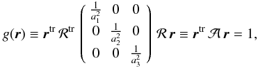 (B.2)
(B.2)
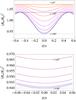 |
Fig. B.1 Normalized projected area of the planet as a function of its anomaly (φ) for inclinations of the orbit going from i = 90° (lowest curve) to i = 0° (highest curve) in steps of 10◦ (5◦ for bottom panel) for a WASP-12 b analog on a circular orbit. Top: for the full orbit. Bottom: zoom on the (primary or secondary) transit. The ordinates of the dotted, solid, and dashed horizontal lines are |


where ℛ is the rotation matrix between the aforedescribed system and the coordinate system attached to the ellipsoid, and the ai are the principal axes of the ellipsoid. In the general case,  takes the form
 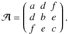 (B.3)The equation of the contour of the projected shadow is given by the fact that the normal to the ellipsoid is normal to the line of sight at this location. This reads as
 ![Mathematical equation: \appendix \setcounter{section}{2} \begin{eqnarray} 0=\mathbf{grad} [g(\vr)]^\mathrm{tr} \cdot \vec{\hat{x}}=2 \,\vr^\mathrm{tr}\, \mathcal{A}\,\vec{\hat{x}}. \end{eqnarray}](/articles/aa/full_html/2011/12/aa15811e-10/aa15811e-10-eq17.png) (B.4)This shows that these points are located on a plane whose equation is (since a ≠ 0)
(B.4)This shows that these points are located on a plane whose equation is (since a ≠ 0) 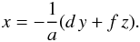 (B.5)This equation differs from Eq. (B.6) in Leconte et al. by the minus sign that was formerly omitted, which slightly changes Eqs. (B.6) and (B.7). Substituting x in Eq. (B.2) by Eq. (B.5) we see that the cross section is an ellipse following the equation
 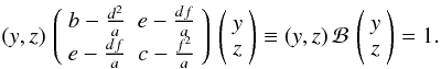 (B.6)It is thus possible to find the rotation in the sky plane needed to reduce the ellipse and find its principal axes (p1, p2). If only the cross section (πp1p2) is needed, we can use that the determinant of a matrix is independent of the coordinate system so that
 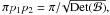 with
with 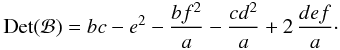 (B.7)
(B.7)
B.2. Coplanar case
We consider the case where the planet equator and the orbital plane are coplanar. If i is the inclination of the orbit with respect to the sky plane and φ the true anomaly defined to be 0 at the instant of inferior conjunction, the rotation matrix reads as 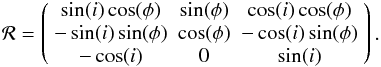 (B.8)The matrix can be computed thanks to Eq. (B.2) giving the a, b, ..., f coefficients and thus Det(ℬ). This gives the projected area of the planet or the star at any given point of the orbit
  (B.9)as shown in Fig. B.1. However, this formula is more general. It is also the cross section that would be seen by an observer located in the direction
  (B.10)in the reference frame defined by the three main axes of the ellipsoid (see Appendix B of Leconte et al. for details).
© ESO, 2011
All Figures
|
Fig. B.1 Normalized projected area of the planet as a function of its anomaly (φ) for inclinations of the orbit going from i = 90° (lowest curve) to i = 0° (highest curve) in steps of 10◦ (5◦ for bottom panel) for a WASP-12 b analog on a circular orbit. Top: for the full orbit. Bottom: zoom on the (primary or secondary) transit. The ordinates of the dotted, solid, and dashed horizontal lines are |
| In the text | |
Current usage metrics show cumulative count of Article Views (full-text article views including HTML views, PDF and ePub downloads, according to the available data) and Abstracts Views on Vision4Press platform.
Data correspond to usage on the plateform after 2015. The current usage metrics is available 48-96 hours after online publication and is updated daily on week days.
Initial download of the metrics may take a while.