© ESO, 2011

1. Introduction

The growth of galaxies via the accretion of smaller companion systems is one of the major ingredients in the current perception of galaxy formation and evolution. These satellite galaxies are disrupted in the tidal field of their host galaxies, and the new material is dispersed near the orbit of the progenitor. Recent theoretical work has shown that especially the outer stellar halo is mainly made of stars that were born outside the main galaxy (Abadi et al. 2006; Zolotov et al. 2009; Scannapieco et al. 2011). Such stars are thought to have low metallicities and to be old. The small fraction of material born inside the main galaxy reaching these large radii was mostly re-distributed during violent major merger events. As these events were more frequent when the galaxy was still young, these stars are also predominantly old. A third small population of the outer halo are the so-called hypervelocity stars (HVSs) which are ejected via a three-body interaction involving the supermassive black hole (SMBH) in the Galactic center (Hills 1988). Such stars have no age constraints and should be metal-rich since they originate in the innermost region of the galaxy.

This population has earned attention since they can serve as an indirect proof that an SMBH is in the Galactic center (Hills 1988) and also because they can be used to measure the shape of the Galactic potential (Gnedin et al. 2005; Yu & Madau 2007; Perets et al. 2009). Yu & Tremaine (2003) estimated an HVS ejection rate of 10^-5 yr^-1, and Perets et al. (2007) show that this rate could increase by a magnitude if massive perturbers, such as giant molecular clouds or star clusters, were considered. Aside from the classical ejection mechanism by Hills (1988), several authors have suggested alternative formation scenarios: a binary black hole of equal (Yu & Tremaine 2003) and unequal masses (Levin 2006; Sesana et al. 2009) or the accretion of a satellite galaxy (Abadi et al. 2009).

Recent observations of 17 stars in the Galactic halo with unusually high velocities (Brown et al. 2005; Hirsch et al. 2005; Edelmann et al. 2005; Brown et al. 2006a,b, 2007a,b, 2009a; Tillich et al. 2009) have raised new interest in the topic. By the design of the search strategy, these stars typically have blue colors. They move with velocities up to 720 km s^-1 with respect to the Galactic center and are thought to reside at Galactocentric distances of 20–130 kpc. Interestingly, the targeted HVS survey of Brown et al. (2009a) only yield outgoing HVSs, which are typically attributed to the short lifetimes of the stars compared to the long orbital periods. However, eventually an ingoing star with extremely high velocity was also observed (Przybilla et al. 2010a).

Despite the small number of HVSs reported to date, several peculiarities in the distribution of the observed population have already been claimed. Abadi et al. (2009) find that a large part of the population clusters around a certain travel time (~130 Myr), i.e. the time a star would need to travel from the GC and arrive at its current radius with its current radial velocity. Such a clustering is not expected from Hills’ original SMBH-ejection scenario. It could be explained, however, by a starburst event near the GC triggering an increased ejection rate of HVSs for certain times.

In addition, the angular distribution on the sky shows signs of anisotropy. Abadi et al. (2009) and Brown et al. (2009b) report a significant overdensity of HVSs around the constellation of Leo. Stars ejected by one or more black holes in the GC should appear on the sky in an approximately homogeneous distribution or in a ring-like structure (Levin 2006). However, a preferred ejection direction as found in the data is not naturally explained with this mechanism (however, see Lu et al. 2010).

The accreted population of stars in the outer halo can also contain stars with high radial velocities. Teyssier et al. (2009) show that there should be an energetically loosely or unbound population of stars originating in disrupted dwarf galaxies. Abadi et al. (2009) comment that a higher total mass of the Galaxy would allow the normal virialized halo population to reach these velocity regimes. The authors further suggest that the peculiarities in the HVS distribution would be naturally explained if part of the observed HVSs actually belonged to a stream of tidal debris of a recently accreted dwarf galaxy. An example of an HVS likely being generated by this mechanism has recently been found in M 31 (Caldwell et al. 2010).

Several theoretical studies have already investigated properties of the tidal debris of satellite galaxies. Johnston (1998) approximated the energy distribution of tidal debris particles with a triangular shape to build up a stellar halo distribution. Choi et al. (2007) show that the energy kick obtained by stripped stars via tidal forces and also the deviations between leading and trailing tidal arms both increase with the mass of the approaching satellite. Warnick et al. (2008) investigated the relation between observable properties of tidal streams like radial velocity dispersion or thickness to the properties of the progenitor system. D’Onghia et al. (2009, 2010) investigated the effect of resonances during tidal stripping of rotating systems.

In the present work we investigate the kinematical properties of tidal debris with a special focus on the fastest stars of this population. For this we systematically studied tidal encounters of satellite galaxies with their hosts to comprehensively investigate the process. We ran a suite of collisionless N-body simulations following the passage of a small companion galaxy through its massive Milky Way-like host galaxy. The set-up of these simulations is described in Sect. 2. In Sect. 3 we analyze these simulations to obtain an idea of what properties an observer would find in an HVS population generated in a tidal collision. Then a simple analytical model is developed and tested against the simulations (Sect. 4). We show in Sect. 5 how this model can be used to predict the energy distribution of the tidal debris star. In Sect. 6 we discuss our results and summarize them in Sect. 7.

2. Simulation set-up

All simulations were run using the publicly available simulation code Gadget-2 (Springel 2005). For the main galaxy we used the model parameters proposed by Klypin et al. (2002). The galaxy consists of three components, an adiabatically contracted spherical NFW halo (Navarro et al. 1997), an exponential stellar disk and a spherical stellar bulge with a Hernquist density profile (Hernquist 1990). The disk density profile is ${\mathit{\rho }}_{\mathrm{disk}}\mathrm{\left(}\mathit{R,z}\mathrm{\right)}\mathrm{=}\frac{{\mathit{M}}_{\mathrm{disk}}}{\mathrm{4}\mathit{\pi }{\mathit{R}}_{\mathrm{disk}}^{\mathrm{2}}{\mathit{z}}_{\mathrm{disk}}}\exp \left(\mathrm{-}\frac{\mathit{R}}{{\mathit{R}}_{\mathrm{disk}}}\right){\mathrm{sech}}^{\mathrm{2}}\left(\frac{\mathit{z}}{{\mathit{z}}_{\mathrm{disk}}}\right)\mathit{,}$(1)where $\mathit{R}\mathrm{=}\sqrt{{\mathit{x}}^{\mathrm{2}}\mathrm{+}{\mathit{y}}^{\mathrm{2}}}$. The vertical scale height is set as z_disk = 0.2R_disk, as was found in observations of other disk galaxies (Kregel et al. 2002). Table 1 presents the parameters used.

The satellite galaxies are modeled as an adiabatically contracted NFW halo hosting a Hernquist sphere as the spherical baryonic component. The models fulfill the constraints from the Fundamental plane of dE+dSph galaxies given in de Rijcke et al. (2005): $\begin{array}{ccc}\log {\mathit{L}}_{\mathit{B}}& \mathrm{~}\mathrm{4.39}\mathrm{+}\mathrm{2.55}\log {\mathit{\sigma }}_{\mathrm{0}}& \\ \log {\mathit{L}}_{\mathit{B}}& \mathrm{~}\mathrm{8.69}\mathrm{+}\mathrm{3.55}\log {\mathit{R}}_{\mathrm{e}}\mathit{.}& \end{array}$Here, L_B is the B-band luminosity, R_e is the effective radius enclosing half the light of the galaxy and σ₀ is the luminosity-weighted mean velocity dispersion. A Hernquist sphere has an effective radius R_e ≃ 1.82r_bulge (Hernquist 1990). For the velocity dispersion σ₀, in analogy to the dispersion used by de Rijcke et al. (2005), we computed the mass-weighted mean of the line-of-sight velocity dispersions in different radial annuli of the visible component. Finally, to relate the luminosity L_B to the baryonic mass content of the galaxy we assume a mass-to-light ratio Υ_B = 2Υ_B, ⊙ .

The ratio between total, M_sat, and baryonic mass, M_sat,b, was fixed using the relation found by McGaugh et al. (2010): $\log {\mathit{M}}_{\mathrm{sat}\mathit{,}\mathrm{b}}\mathrm{=}\mathrm{4.0}\log {\mathit{v}}_{\mathrm{circ}}\mathrm{+}\mathrm{1.65.}$(4)To relate the circular velocity of the dark halo, v_circ, to the mass of the satellite, M_sat, we used the same relation as in McGaugh et al. (2010): ${\mathit{M}}_{\mathrm{sat}}\mathrm{=}\mathrm{(}\mathrm{1.5}\mathrm{\times }{\mathrm{10}}^{\mathrm{5}}{\mathrm{km}}^{-3}{\mathrm{s}}^{\mathrm{3}}{\mathit{M}}_{\mathrm{\odot }}\mathrm{)}{\mathit{v}}_{\mathrm{circ}}^{\mathrm{3}}\mathit{.}$(5)With these constraints the dwarf galaxy is fully determined by only one parameter. In this work we used the total mass M_sat as a free parameter that was varied for different simulation runs. The requirement to match all the constraints given above also fixes the concentration parameter c of the satellite dark halo. The obtained mass-concentration relation is given in Fig. 1. It is best described by a power law: $\mathit{c}\mathrm{\simeq }\mathrm{19.3}{\left(\frac{{\mathit{M}}_{\mathrm{sat}}}{{\mathrm{10}}^{\mathrm{10}}{\mathit{M}}_{\mathrm{\odot }}}\right)}^{\mathrm{0.36}}\mathrm{·}$(6)This relation was obtained by fitting our basic satellite model to the observational constraints. Our concentration parameter should thus not be interpreted in the original sense of an evolutionary sequence in the framework of ΛCDM cosmology (Navarro et al. 1997).

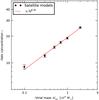Fig. 1 Relation between the concentration parameter c of the dark halo and the total mass of the satellites. The black symbols show the applied values for the halo concentration parameter c for a given satellite mass Msat. The errorbars have a width of 0.5 to reflect that only integer numbers were used for c. The red line shows a power law with exponent 0.36.

For initializing of the phase-space positions of the particle samples, we followed a method outlined by Springel & White (1999), which is a modified version of the method of Hernquist (1993) that assumes Gaussian velocity distributions. The latter leads to slight deviations from a perfect equilibrium configuration. To account for this, both host and satellite galaxies are allowed to relax for 1 Gyr in isolation before they are implemented into the actual simulations. We used a softening length of 0.01 (0.2) kpc for the satellite star (dark matter) particles in all our simulations.

Simulation time

All simulations ran until the satellite reached the apogalacticon after its first pericentric passage or crossed the virial radius of the host galaxy, R₂₀₀. This was done because we wanted to study the properties of a population of tidal debris particles generated during a single stripping event. As we also have a focus on the stars escaping from the combined satellite and host system, we chose to study only the first orbit. We expect this orbit to generate the widest spread in velocities because the initial unperturbed satellite population covers the complete possible phase space region. At later orbits the satellite will have lost its most energetic population (Choi et al. 2009). Furthermore, considering only the first orbit allows an easier comparison between the different simulation runs because one has the full control over the satellite configuration at the beginning of the orbit.

A suite of simulations

To create a suite of comparable simulations we then ran this scenario with varying initial satellite masses M_sat = 0.1 − 2 × 10¹⁰M_⊙ and different starting positions in the satellite phase space. In the majority of cases, the satellite is on a bound polar orbit with respect to the host disk component. To determine the influence of an inclined orbit we also ran a couple of simulations with 0° (planar) and 45° inclination angle. We found that the differences in the results for varying inclinations were small compared to other uncertainties. We thus did not consider inclination as a major parameter and neglected it completely. The initial angular momenta, L_sat, of the satellites range between 0 and 15 × 10³ kpc km s^-1, which corresponds to pericenter distances R_peri from 0 to 50 kpc. Table D.1 lists the initial conditions and some of the analysis results for all runs.

3. Observable properties from the simulations

Of the 41 simulations performed for this study 23 yielded particles with velocities higher than the local escape speed of the host galaxy. These particles are gravitationally unbound and are the simulated equivalent to HVSs. However, in the real Milky Way the escape speed is still uncertain to a considerable degree since neither the total mass (1 − 2 × 10¹²M_⊙, e.g. Smith et al. 2007; Xue et al. 2008; Guo et al. 2010; Boylan-Kolchin et al. 2011; Przybilla et al. 2010b) nor the global shape of the gravitational potential (Law et al. 2009) is measured accurately. Moreover, the asymmetry of the Galaxy introduces a direction dependency. Thus the value of the escape speed must not be seen as a sharp limiting velocity dividing bound and unbound stars. It is instead a characteristic value to compare to when evaluating the probability of whether a star will eventually fall back onto its host or not. For the dynamics of a star located within the virial radius of the Galaxy, it makes no qualitative difference whether it is gravitationally unbound. Because of this, to obtain higher quality statistics, we thus in this section analyze the most energetic 0.1% of the satellite particles, i.e. the most energetic particles (MEPs, for short) regardless of whether they reach velocities higher than their local escape speed.

Angular distribution

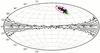Fig. 2 Aitoff projection of a simulation run about 200 Myr after perigalacticon. Green dots represent all satellite particles (only every 5th particle is plotted), while the MEPs are marked by red stars. The disk and bulge of the host galaxy are also shown as black mass-density contour lines. The median distance of the MEPs is  ~ 60 kpc, comparable to the Galactocentric distances of the observed HVSs. The MEPs are concentrated to confined area on the sky, in this case enclosed by a circle with angular radius 15°.

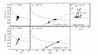Fig. 3 Time series of the galactocentric RV-distance plane for two simulation runs. The time elapsed since perigalacticon, Δtperi, is shown in the upper left corner. Red stars represent the MEPs, green dots satellite particles, and dashed lines the local escape speed of the respective radius. Dotted lines mark lines of constant travel times corresponding to Δtperi. The eccentricity of the satellite orbit is given in the lower right corner of the rightmost panel. In the leftmost panels the mean distance of the MEPs is 60 kpc similar to the observed HVS population, which is shown in the right most panel in the upper row for comparison. None of the simulations were designed to reproduce the observed HVS population.

Figure 2 shows the angular distribution of the MEPs in one of our simulations as seen by an observer at the Sun’s location. The snapshot is taken at a time when the particles have moved from the satellite perigalacticon out to a galactocentric distance of  ~60 kpc, similar to the observed HVS population. As already reported by Abadi et al. (2009) the MEPs are clustered in a tightly confined region on the sky. Averaging over all 39 simulations and over ten equispaced angular positions of the sun on the solar circle, the mean radius of a circular region encompassing all MEP is 16° and the maximum angular radius is 27°. At a distance of 60 kpc the viewing angle of the observer relative to the orbital plane of the satellite does not play a significant role, because the stripped off particles did not have enough time yet to unfold into a prominent stream and are thus observable in a compact area from all directions (cf. the upper lefthand panel of Fig. 3).

Furthermore, the position of the satellite relative to the MEPs is not arbitrary. In all our simulations the satellite has a smaller angular distance to the host galactic center than the MEPs. This is because both the satellite and the MEPs have just passed their perigalacticon and are now moving away from the host. Since the MEPs have higher orbital energies, they leave the satellite behind and are thus observed at larger angular distances in the vast majority of cases. The angular distance between the MEPs and the satellite remnant is determined by projection effects depending on the viewing angle relative to the orbital plane of the satellite. In our simulations the satellite core is always observed within a 22° (90 percent within 16°) separation to the center of the MEP population.

The radial velocity-distance plane

The particles stripped-off the satellite quickly disperse in physical space and are soon indistinguishable from the already existing Galactic halo population. However, when Galactocentric radial velocities (RVs) are plotted against Galactocentric distance, r, the particles form an elongated pattern reflecting their common origin from the perigalacticon of the satellite. Figure 3 shows time series of two simulations with satellite systems on orbits with different eccentricities. The upper series is based on the same simulation that was used for Fig. 2 and the upper leftmost panel shows the same point in time. The lower panel row shows a simulation run with an almost purely radial orbit, which also has lower orbital energy. The initial structural properties of the satellite are the same as in the upper run. Note that despite the lower satellite orbital energy the maximum tidal debris velocities are larger than in the run with a lower eccentricity.

The radial trend of the escape speed also indicated in the panels corresponds to the trajectory of a test body on a parabolic (purely radial) orbit. Particles below this line are not necessarily bound because part of their motion is hidden in the other velocity components. This explains why particles can cross the dashed line while still conserving their energy.

Lines of constant travel time mark positions in the RV-r-plane that are occupied by test bodies that started from a common point with varying initial (radial) velocities. The starting point is usually chosen to be the center of the gravitational potential, as in Fig. 3. However, lines from other starting points have similar shapes, which explains the good alignment of the tidal debris particles even though the satellite in the upper row run never comes close to the Galactic center. The pericenter distance for this run was 18 kpc.

The width of the tidal debris streams in the RV-r plane also changes with eccentricity. This can be understood when considering that most of the stripping happens during a short period of time around the pericenter passage. For a more circular orbit, this period gets more extended as more time is spent by the satellite at radii similar to the pericenter distance. Because of this, the clustering in travel time already reported by Abadi et al. (2009) has an intrinsic scatter which scales with eccentricity of the orbit of the progenitor system. This is especially the case shortly after the pericentric passage, when the distances to the GC are not large and lines of constant travel times have a steep slope. At this time the scatter can be stronger than the trend to lines of constant travel time.

The leftmost panel (upper row) shows the distribution of the observed HVSs in the distance-velocity plane for comparison. The possible tidal debris group in the population proposed by Abadi et al. (2009) clusters around the 133 Myr-line of constant travel time. Neither of the two simulation runs was designed to reproduce the observed population as this was not the goal of this more general parameter study.

Maximum velocities

In the classical SMBH sling shot scenario the extremely high ejection velocities are a result of the extreme orbital velocities occurring near an SMBH plus the large orbital velocities of the components of a hard binary system (Yu & Tremaine 2003). Compared to such an environment, collisions of galaxies are much less violent events because the time scales are much larger and potential gradients much shallower. We thus cannot expect these extraordinary velocities up to 3000 km s^-1 predicted by Hills (1988). Still, the simulations show that stars can be accelerated to their local escape speed and above. The maximum velocities reached by the MEPs at r ≃ 60 kpc in our simulations range between 200 and 400 km s^-1 (v_esc(60kpc) = 330 km s^-1 in our Galaxy model).

4. A model for tidal stripping

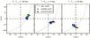Fig. 4 Snapshots of the satellite (small green dots) shortly before, during, and shortly after its pericentric passage. Red stars show the positions of those particles that will have the highest orbital energy at the end of the simulation. Blue triangles show those with the lowest energy.

To guide our further analysis we developed a simple, succinct model to describe the accreted satellite mechanism. It was inspired by the calculations of HVS ejection velocities by Yu & Tremaine (2003) because it treats the galaxy-galaxy encounter in a similar fashion as these authors did for a binary-SMBH encounter: a satellite galaxy is moving on an orbit in the gravitational potential Φ_host(r) of its much more massive host galaxy. Its specific orbital energy is thus 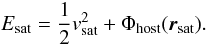${\mathit{E}}_{\mathrm{sat}}\mathrm{=}\frac{\mathrm{1}}{\mathrm{2}}{\mathit{v}}_{\mathrm{sat}}^{\mathrm{2}}\mathrm{+}{\mathrm{\Phi }}_{\mathrm{host}}\mathrm{\left(}{{r}}_{\mathrm{sat}}\mathrm{\right)}\mathit{.}$(7)Since the satellite is a spatially extended object, it is subject to tidal forces that lead to a mass loss of the satellite. Under the assumption of an at least moderately eccentric orbit, the majority of this stripping will happen in a short period of time when the satellite is closest to the center of the host galaxy where tidal torques are strongest, i.e., at its perigalacticon, R_peri, where it has the velocity v_sat = V_peri.

To model the stripping we now assume what we call instantaneous escape: a star i with a position r_i relative to the satellite center and a velocity v_i in the comoving rest frame of satellite has an orbital energy 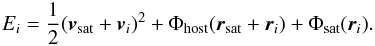${\mathit{E}}_{\mathit{i}}\mathrm{=}\frac{\mathrm{1}}{\mathrm{2}}\mathrm{(}{{v}}_{\mathrm{sat}}\mathrm{+}{{v}}_{\mathit{i}}{\mathrm{)}}^{\mathrm{2}}\mathrm{+}{\mathrm{\Phi }}_{\mathrm{host}}\mathrm{(}{{r}}_{\mathrm{sat}}\mathrm{+}{{r}}_{\mathit{i}}\mathrm{)}\mathrm{+}{\mathrm{\Phi }}_{\mathrm{sat}}\mathrm{(}{{r}}_{\mathit{i}}\mathrm{)}\mathit{.}$(8)It is lost to the satellite when the gravitational potential from the satellite, Φ_sat is less than the difference in the host potential between the satellite position and the position of the particle, r_i, ${\mathrm{\Phi }}_{\mathrm{host}}\mathrm{(}{{r}}_{\mathrm{sat}}\mathrm{+}{{r}}_{\mathit{i}}\mathrm{)}\mathrm{-}{\mathrm{\Phi }}_{\mathrm{host}}\mathrm{\left(}{{r}}_{\mathrm{sat}}\mathrm{\right)}\mathrm{\ge }\mathrm{-}{\mathrm{\Phi }}_{\mathrm{sat}}\mathrm{\left(}{{r}}_{\mathit{i}}\mathrm{\right)}\mathit{,}$(9)which is equivalent for it to be outside of the tidal radius, R_tidal. We now assume that this energy transition occurs instantly, and the star is left to move in the host potential only. Thus the orbital energy of the star after the stripping is $\begin{array}{ccc}{\mathit{E}}_{\mathit{i}}^{\mathrm{\prime }}& \mathrm{=}& \frac{\mathrm{1}}{\mathrm{2}}\mathrm{(}{{v}}_{\mathrm{sat}}\mathrm{+}{{v}}_{\mathit{i}}{\mathrm{)}}^{\mathrm{2}}\mathrm{+}{\mathrm{\Phi }}_{\mathrm{host}}\mathrm{(}{{r}}_{\mathrm{sat}}\mathrm{)}\mathrm{=}\\ & \mathrm{=}& {{v}}_{\mathrm{sat}}{{v}}_{\mathit{i}}\mathrm{+}\frac{\mathrm{1}}{\mathrm{2}}{\mathit{v}}_{\mathit{i}}^{\mathrm{2}}\mathrm{+}\frac{\mathrm{1}}{\mathrm{2}}{\mathit{v}}_{\mathrm{sat}}^{\mathrm{2}}\mathrm{+}{\mathrm{\Phi }}_{\mathrm{host}}\mathrm{\left(}{{r}}_{\mathrm{sat}}\mathrm{\right)}\mathrm{=}\\ & \mathrm{=}& {{v}}_{\mathrm{sat}}{{v}}_{\mathit{i}}\mathrm{+}\frac{\mathrm{1}}{\mathrm{2}}{\mathit{v}}_{\mathit{i}}^{\mathrm{2}}\mathrm{+}{\mathit{E}}_{\mathrm{sat}}\mathit{.}\end{array}$(10)The energy kick obtained by the star compared to the satellite is then $\mathrm{\Delta }{\mathit{E}}_{\mathit{i}}\mathrm{=}{{v}}_{\mathrm{sat}}{{v}}_{\mathit{i}}\mathrm{+}\frac{\mathrm{1}}{\mathrm{2}}{\mathit{v}}_{\mathit{i}}^{\mathrm{2}}\mathit{.}$(11)We now ask for the maximum of ΔE. Equation (11) leads to the assumption that three conditions need to be fulfilled for the maximum energy kick.

• 1.

  The star has the maximum velocity possiblewhich is the local escape speed at the tidal radius:v_i = v_esc(R_tidal).

• 2.

  Satellite and stellar velocities have to be aligned: v_sat||v_i.

• 3.

  The satellite has to be at its maximum velocity, which occurs during the passage of the Perigalacticon: v_sat = V_peri.

Moreover, if the star is to gain orbital energy, it needs to be at larger Galactocentric radii than the satellite, i.e.  | r_sat + r_i |  > r_sat, because only then does the tidal force push the star away from the galactic center, hence from the potential well. This, together with the first condition, requires the star to be on a prograde orbit with respect to the satellite motion. This view is also confirmed by Fig. 4. It shows three snapshots of a simulation run shortly before, at, and shortly after perigalacticon. Those particles that will have the highest and lowest orbital energy at the end of the simulation are situated are very distinct locations with respect to the satellite. The particles that gain energy move along with the satellite on an orbit, that is prograde with respect to the satellite motion, while for particles that lose energy the orbital phase is such that their motion opposite to the direction of the system velocity.

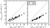Fig. 5 Energy gain with respect to Esat predicted by our simplified model ΔEmax compared to the maximum energy gain found in each simulation. The latter are by a factor of  ~0.45 (slope of the gray dotted lines) lower than the estimates, which is most likely due to oversimplification of the model. Phase-space sampling due to the limited particle number does not play a significant role as can be seen from the gray circles thAT mark the runs with 10 times lower resolution. Left: the estimated energy gain as obtained from our model. Right: the energy gain from our model corrected for an additional dependency on the angular momentum of the satellite. See text for a discussion.

Thus we arrive at $\mathrm{\Delta }{\mathit{E}}_{\max }\mathrm{=}{\mathit{V}}_{\mathrm{peri}}{\mathit{v}}_{\mathrm{esc}}\mathrm{\left(}{\mathit{R}}_{\mathrm{tidal}}\mathrm{\right)}\mathrm{+}\frac{\mathrm{1}}{\mathrm{2}}{\mathit{v}}_{\mathrm{esc}}\mathrm{(}{\mathit{R}}_{\mathrm{tidal}}{\mathrm{)}}^{\mathrm{2}}\mathit{.}$(12)In the lefthand panel of Fig. 5 we compare this model prediction obtained from Eq. (12) to simulation results. For the latter the particle with the highest orbital energy max(E_i) was identified when the satellite remnant reached apogalacticon after the first passage through the host system. The energy gain ΔE_max,sim is then defined as max(E_i) − E_sat. For further details of how this estimate was done we refer the reader to Appendix A. Equation (12) systematically overestimates the maximum energy kick by a (constant) factor of 2.2, as indicated by the positions of the points in Fig. 5 on a line with slope α = 2.2^-1 ≃ 0.45. The overestimation is most likely due to oversimplification of our estimate, e.g. the neglect of the structural evolution of the satellite in the tidal field. Surprisingly, the mass resolution only plays a minor role in the sense that simulation runs with lower particle numbers do not yield significantly smaller maximum energy differences. This is most likely due to the steep slope of the energy distribution of the tidal debris stars (see Sect. 5 and Fig. B.1).

Much of the scatter in the lefthand panel of Fig. 5 turned out to be a residual dependency on the initial angular momentum of the respective satellites in the simulation. We obtain a tighter relation (righthand panel) when we use $\mathrm{\Delta }{\mathit{E}}_{\max \mathit{,}\mathrm{c}}\mathrm{=}\mathrm{\Delta }{\mathit{E}}_{\max }\sqrt{\frac{{\mathit{L}}_{\mathrm{sat}}\mathrm{+}{\mathit{L}}_{\mathrm{char}}}{{\mathit{L}}_{\mathrm{char}}}}\mathit{,}$(13)with L_char = 6300 kpc km s^-1. Thus the value αΔE_max,c gives a robust estimate of the maximum energy gain occurring during a satellite-host galaxy encounter.

Dynamical friction

In the course of its orbit the satellite galaxy is also subject to dynamical friction. This means that it will sink deeper into the potential well of the host system. By the time it reaches its perigalacticon stripped-off stars might have to get over a much wider energy gap to become HVSs. The extent of the energy loss depends mainly on the mass M_sat and the orbit of the satellite, in a way that is counterproductive to the ejection energies ΔE_max: a more massive satellite ejects stars at higher energies since its internal velocities are higher. This energy gain for the stripped-off stars scales roughly with $\sqrt{{\mathit{M}}_{\mathrm{sat}}}$ since ${\mathit{v}}_{\mathrm{esc}}\mathrm{\left(}\mathit{r}\mathrm{\right)}\mathrm{\propto }\sqrt{{\mathit{M}}_{\mathrm{sat}}}$, which goes into our estimate (Eq. (12)). On the other hand, a higher mass results in stronger dynamical friction which roughly scales  ∝ M_sat (Chandrasekhar 1943). In fact in our simulations we find that the loss in orbital energy after one orbit is $\mathrm{\Delta }{\mathit{E}}_{\mathrm{DF}}\mathrm{=}\mathrm{2}\mathrm{\times }{\mathrm{10}}^{-4}{\left(\frac{{\mathit{M}}_{\mathrm{sat}}}{{\mathit{M}}_{\mathrm{\odot }}}\right)}^{\mathrm{0.78}}{\left(\mathrm{1}\mathrm{+}\frac{{\mathit{L}}_{\mathrm{0}}}{\mathrm{5900}{\mathrm{kpc}\mathrm{km}\mathrm{s}}^{-1}}\right)}^{-1}\mathit{,}$(14)which reflects the dependence of the physical extent of the satellite on its mass and also the change of the orbital trajectories with changing orbital angular momentum. We use this simplistic approach as it best covers the effect of a possible reaction of the host galaxy on the intruder (however, see Taylor & Babul (2001) and Gan et al. (2010) for a more detailed approach to model dynamical friction).

Above a certain mass the satellite will therefore not be able to eject any HVSs since the energy loss of the whole system is greater than the energy gain of the single stars. However, judging from our simulations, this will only happen at masses  > 10¹¹M_⊙. Extrapolating our results into this (major merger) mass regime is not meaningful, since a massive intruder will significantly perturb the host galaxy. We can thus just state that this scenario does not occur for minor mergers in the present work.

Hypervelocity stars

In the context of hypervelocity stars that are unbound to the total system we have to compare ΔE with E_sat, the orbital energy of the satellite, since the energy E of such an unbound object must be $\mathit{E}\mathrm{=}{\mathit{E}}_{\mathrm{sat}}\mathrm{-}\mathrm{\Delta }{\mathit{E}}_{\mathrm{DF}}\mathrm{+}\mathrm{\Delta }\mathit{E}\mathrm{\ge }\mathrm{0.}$(15)Thus the condition $\mathit{\alpha }\mathrm{\Delta }{\mathit{E}}_{\max \mathit{,}\mathrm{c}}\mathrm{\ge }\mathrm{-}{\mathit{E}}_{\mathrm{sat}}\mathrm{+}\mathrm{\Delta }{\mathit{E}}_{\mathrm{DF}}\mathit{.}$(16)must be fullfilled to allow unbound stars to be generated during such a satellite-host galaxy encounter with α ≃ 0.45.

5. The energy distribution

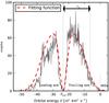Fig. 6 A histogram of the orbital energies of all particles that initially belonged to the satellite but became unbound to it in the course of the first orbit (tidal debris particles). The two peaks correspond to the two tidal arms torn out of the satellite. The central gap coincides with the orbital energy Esat of the remaining satellite system. The dashed red line shows the fitting function (Eq. (17)), which is used to characterize the distribution. The meaning of the fitting parameter ϵw, which is used to determine the width of the high energy peak, is also indicated.

A more robust measure of the range of orbital energies covered by the stripped-off stars can be obtained when looking at the overall width of the energy distribution of all particles gravitationally unbound to the satellite. We determine these stars using an iterative method described by Tormen et al. (1998). The energy distribution is plotted in Fig. 6. The two peaks represent the leading and trailing tidal arm, respectively. The gap between them is centered on the orbital energy of the satellite. We apply an empirical fitting function ${\mathit{f}}_{\mathrm{fit}}\mathrm{\left(}\mathit{E}\mathrm{\right)}\mathrm{=}\frac{{\mathit{f}}_{\mathrm{high}}}{\mathit{C}}\left[\frac{\mathrm{1}}{(\mathrm{1}\mathrm{+}\exp (\mathit{\gamma }(\frac{\mathrm{\Delta }\mathit{E}}{{\mathit{ϵ}}_{\mathrm{w}}}\mathrm{-}\mathrm{1})){)}^{\mathrm{2}}}\mathrm{-}{\mathit{f}}_{\mathrm{inner}}\exp \left(\mathrm{-}{\left(\frac{\mathrm{\Delta }\mathit{E}}{{\mathit{ϵ}}_{\mathrm{inner}}}\right)}^{\mathrm{2}}\right)\right]\mathit{,}$(17)again with ΔE = E − E_sat. To normalize the function we use the factor f_high/C, where f_high is the number of particles in the high-energy (trailing) arm divided by the initial number of satellite particles and $\begin{array}{c}\\ \mathit{C}& \mathrm{=}\frac{\mathrm{1}}{{\mathit{f}}_{\mathrm{high}}}{\mathrm{\int }}_{{\mathit{E}}_{\mathrm{sat}}}^{\mathrm{\infty }}{\mathit{f}}_{\mathrm{fit}}\mathrm{\left(}\mathit{E}\mathrm{\right)}\mathrm{d}\mathit{E}\\ & \mathrm{=}{\mathit{ϵ}}_{\mathrm{w}}\left[\mathrm{1}\mathrm{+}\frac{\mathrm{1}}{\mathit{\gamma }}\left(\ln \mathrm{(}\mathrm{1}\mathrm{+}{\mathrm{e}}^{\mathrm{-}\mathit{\gamma }}\mathrm{)}\mathrm{-}\frac{\mathrm{1}}{\mathrm{1}\mathrm{+}\exp \mathrm{(}\mathrm{-}\mathit{\gamma }\mathrm{)}}\right)\right]\mathrm{-}\frac{\sqrt{\mathit{\pi }}{\mathit{f}}_{\mathrm{inner}}{\mathit{ϵ}}_{\mathrm{inner}}}{\mathrm{2}}\mathrm{·}\end{array}$(18)The function is shown in Fig. 6. For the fitting procedure we only consider the high energy peak of the distribution, i.e. where E ≥ E_sat. The fitting parameters provide us with some characteristics of respective distribution: the width or typical energy, ϵ_w, the width of the central minimum, ϵ_inner, a measure of how fast the distribution drops off with increasing energy, γ, and the relative depth of the central minimum, f_inner.

A composite distribution

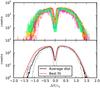Fig. 7 Upper panel: histograms of the energy differences ΔE = Ei − Esat of the tidal debris particles of all simulations used in this work overplotted. The distributions are plotted as functions of ΔE in units of the width of the high-energy peak ϵw. The histograms are also renormalized so that the high energy peak covers the same area. The lines are color-coded according to the initial angular momentum of the progenitor system (from red representing more radial orbits to blue for more circular orbits). Lower panel: the mean distribution obtained from the distribution plotted in the upper panel (solid black line). The standard deviation is also indicated with the thin gray lines. Overplotted in red is our fitting function using the parameters given in Eqs. (20) and ϵw = 1.

Following an idea by Johnston (1998) we assume the general shape of the distributions to be invariant and only the width and the normalization to be specific to the respective orbit and satellite parameters. This means that the parameters ϵ_inner,γ,f_inner are either constant for all situations or a function of ϵ_w. To compare the distribution shapes we rescaled the particle energies into units of their specific typical energy ϵ_w via 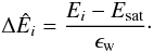$\mathrm{\Delta }\mathit{Ê}\mathit{i}\mathrm{=}\frac{{\mathit{E}}_{\mathit{i}}\mathrm{-}{\mathit{E}}_{\mathrm{sat}}}{{\mathit{ϵ}}_{\mathrm{w}}}\mathrm{·}$(19)The resulting energy distributions were then renormalized to eliminate the influence of the number particles in the respective (trailing) tidal arm. The upper panel of Fig. 7 overplots the energy distributions of all our simulations. These include satellite varying over more than a magnitude in mass and angular momentum. The resulting mean distribution with the standard deviation is also plotted. Applying our fitting function Eq. (17) results in the following parameter values: $\begin{array}{ccc}{\mathit{ϵ}}_{\mathrm{inner}}& \mathrm{=}& \mathrm{0.14}{\mathit{ϵ}}_{\mathrm{w}}\mathit{,}\\ \mathit{\gamma }& \mathrm{=}& \mathrm{5.21}\mathit{,}\\ {\mathit{f}}_{\mathrm{inner}}& \mathrm{=}& \mathrm{0.94.}\end{array}$(20)The fit is shown in Fig. 7. We then repeat the fitting procedure for all single distributions with only ϵ_w as a free parameter. The resulting widths are plotted in Fig. 8 against the highest energy of all satellite particles, ΔE_max,sim. The tight correlation $\mathrm{\Delta }{\mathit{E}}_{\max \mathit{,}\mathrm{sim}}\mathrm{=}\mathit{\beta }{\mathit{ϵ}}_{\mathrm{w}}$(21)with β ≃ 1.5 (which is not strongly affected by the resolution in the simulations) is a result of the steep drop at the high-energy tip of the distribution. Using the simple model developed in the previous section we can thus obtain an estimate for the width of the high-energy peak via $\begin{array}{ccc}{\mathit{ϵ}}_{\mathrm{w}}& \mathrm{=}& {\mathit{\beta }}^{-1}\mathrm{\Delta }{\mathit{E}}_{\max \mathit{,}\mathrm{sim}}\mathrm{\simeq }\frac{\mathit{\alpha }}{\mathit{\beta }}\mathrm{\Delta }{\mathit{E}}_{\max \mathit{,}\mathrm{c}}\\ & \mathrm{=}& \mathrm{0.3}\mathrm{\Delta }{\mathit{E}}_{\max \mathit{,}\mathrm{c}}\mathit{.}\end{array}$(22)Note that v_esc(r) is a proxy for the mass of the satellite. Thus more massive satellites will produce a wider energy spread in the stripped-off stars. One could also say that the higher velocity dispersion of a more massive galaxy directly translates into a larger energy dispersion in the tidal debris.

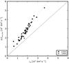Fig. 8 Relation between the maximum energy gain ΔEmax,sim and the width ϵw of the energy distribution of all tidal debris stars obtain via fitting Eq. (17). The gray dotted line has a slope of 1.5.

6. Discussion

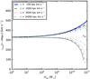Fig. 9 The maximum ejection velocities at a galactocentric distance of 60 kpc as a function of initial satellite mass as computed from Eq. (23) assuming an initial orbital energy of the satellite Esat = 0 km2 s-2. The energy loss due to dynamical friction was computed using the empirical law (Eq. (14)) obtained from our simulations. The lower gray lines show the velocity of the satellite remnant at the same distance.

It is now a straightforward matter to compute the maximum velocities generated during a tidal collision at certain galactocentric radius r > R_peri: $\begin{array}{ccc}{\mathit{v}}_{\max }\mathrm{\left(}\mathit{r}\mathrm{\right)}& \mathrm{=}& {\left[\mathrm{2}\mathrm{(}{\mathit{E}}_{\max }\mathrm{-}{\mathrm{\Phi }}_{\mathrm{host}}\mathrm{(}\mathit{r}\mathrm{\left)}\mathrm{\right)}\right]}^{\frac{\mathrm{1}}{\mathrm{2}}}\\ & \mathrm{=}& {\mathrm{[}{\mathrm{2}\mathrm{(}{\mathit{E}}_{\mathrm{sat}\mathit{,}\mathrm{apo}}\mathrm{+}\mathrm{0.45}\mathrm{\Delta }{\mathit{E}}_{\max \mathit{,}\mathrm{c}}\mathrm{-}{\mathrm{\Phi }}_{\mathrm{host}}\mathrm{(}\mathit{r}\mathrm{\left)}\mathrm{\right)}}^{\mathrm{]}}}^{\frac{\mathrm{1}}{\mathrm{2}}}\mathit{,}\end{array}$(23)where E_sat,apo = E_sat − ΔE_DF is the orbital energy of the remaining satellite after the passage. To obtain a quantitative idea we again assume a Galactocentric distance of r = 60 kpc to be comparable to the observations of HVSs. For the energy loss via dynamical friction ΔE_DF, we use the loss law (Eq. (14)) found in our simulations for simplicity. The velocities obtained in this way are plotted in Fig. 9 as a function of the initial satellite mass M_sat and for four different initial angular momenta L_sat. The satellite system was assumed to approach the host galaxy on a parabolic orbit; i.e., E_sat = 0 km² s^-2. Only the most massive satellite galaxies eject HVSs with substantial velocities comparable to the radial velocities of the observed HVSs. Less massive galaxies could, in principal, also yield such high velocities if they move on more energetic orbits themselves. For example, a satellite with mass M_sat = 10⁹M_⊙ would have to cross the virial radius of our parent galaxy¹ with a velocity of  ~660 km s^-1 to eject a star with 720 km s^-1 at 60 kpc comparable to the fastest HVSs known. Such a system would not lose enough energy to become bound to the larger galaxy. In this case one hardly would speak about an ejected star since the galaxy would move along with the star for a long period of time.

We now consider the subsample of observed HVSs with travel times  ~133 Myr pointed out by Abadi et al. (2009, cf. their Fig. 1). The spread in velocities is roughly² 400 km s^-1. Such strong variations in the velocities translate into a progenitor mass of  ≃ 10¹¹M_⊙. If we select only stars within the overdensity region defined by Abadi et al. (2009) the spread reduces to  ~250 km s^-1 resulting in a minimum progenitor mass still higher than 10¹⁰M_⊙. Concerning the known satellite galaxies the respective authors of the HVS discovery papers have already excluded a kinematical connection to them (Brown et al. 2005, 2006a, 2009a; Edelmann et al. 2005; Hirsch et al. 2005). Since we do not expect such a system to have escaped observations to date, we conclude that a satellite origin for the subsample to be unlikely.

However, one should keep in mind that a more massive host galaxy (our host model has a total mass of 1.1 × 10¹²M_⊙) would shift the lines in Fig. 9 upwards and would, in principal, allow also very small galaxies to produce stars with velocities, e.g.  >500 km s^-1. However, that only massive galaxies can eject stars with significantly higher velocities than their own velocities remains unaffected by this.

The bound HVS population and the outer stellar halo

Several recent studies have shown that the outer stellar halo is almost purely made of accreted stars (Abadi et al. 2006; Zolotov et al. 2009; Scannapieco et al. 2009). As smooth gas accretion via cold flows only plays a minor role for Milky Way-type galaxies at low redshifts (Brooks et al. 2009), we can assume the Galaxy has not grown significantly since its last major merger. Our simulations now demonstrate that satellite accretion will inevitably produce stars with velocities up to and exceeding their local escape speed. This means that the phase space distribution of stellar halo stars reaches all velocities up to the local escape speed at all times. For example, Smith et al. (2007) used this as a critical assumption for their technique to estimate the mass of the Galaxy.

However, this also means that a classification of a star as an HVS ejected from the SMBH based on its velocity is only valid for extremely high velocities. Without a confirmation of their young ages the “bound” HVS population in the compilation of Brown et al. (2009a) is indistinguishable from the normal (accreted) stellar halo population. To date only three stars in the survey have clear spectroscopic identification as main sequence B stars (Fuentes et al. 2006; López-Morales & Bonanos 2008; Przybilla et al. 2008), while others could be old blue stragglers or blue horizontal branch stars (Perets et al. 2009).

An intragalactic stellar population

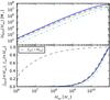Fig. 10 Upper panel: mass ejected at unbound velocities during one satellite orbit as a function of initial progenitor mass. The satellite is assumed to have zero initial orbital energy, i.e. to be on a parabolic orbit. Different lines correspond to four different initial angular momenta of the satellite. The vertical dashed line indicates the mass of a single star particle in our simulations. Lower panel: mass fraction of an unbound intergalactic population originating in satellites with masses below Msat. The fraction were computed using satellite mass function based on the satellite luminosity function of Koposov et al. (2008). The mass function is also shown as a thin dashed line.

With our results we can also address the question of what kinds of satellites are the main contributors to a possible intragalactic stellar population (ISP) or wandering stars (Teyssier et al. 2009). For this we assume the infalling satellite galaxies to be initially on parabolic orbits, i.e. E_sat = 0. Via dynamical friction the satellites will be shifted onto bound orbits during their first passage. Thus not all stars in the trailing (high-energy) tidal arm will become unbound, but only those that gained more energy than is lost by their progenitor system.

By integrating our fitting formula (Eq. (17)) using the proper value for ϵ_w obtained via Eqs. (13) and (21) over higher energies than the frictional energy loss ΔE_DF, we obtain the fraction of the baryonic mass that became HVSs. In the upper panel of Fig. 10, this fraction multiplied by the baryonic mass content of the satellite is shown as a function of the total satellite mass. For the estimation an initial angular momentum L₀ had to be set. The plot shows the results for four different L₀ (color coding as in Fig. 9).

We then convolved this mass ejection function with an observational mass function of dwarf galaxies. We therefore used the luminosity function obtained by Koposov et al. (2008) and converted it into a mass function using the same relations as were used to create our satellite models for the simulations. As a result we obtained the cumulative HVS mass production function shown in the lower panel of Fig. 10. Consistent with the results of Teyssier et al. (2009) obtained via cosmological simulations we find that a tiny minority of massive satellites produces the overwhelming majority of HVSs. Given that more massive galaxies are usually also more metal-rich (Tamura et al. 2001) we conclude that an intragalactic stellar population should have at least on average a higher metalicities than the surviving dwarf galaxy population.

7. Summary

In the present work we have used a suite of 41 N-body simulations to study the tidal debris of satellite galaxies interacting with their much more massive host systems. Abadi et al. (2009) suggest that a fraction of the stripped-off stars can reach significant velocities and could be confused with HVSs ejected from the Galactic center by a supermassive black hole. We found that, as suggested by these authors, the stripped-off stars are in fact observed in a confined region on the sky. However, for stars at distances still observable from the solar position the reason for this is not only the projection of a collimated stellar stream along the line of sight, but in addition that so shortly after the stripping event the stars had not yet enough time to disperse in physical space. We further developed a simple analytic model predicting the maximum possible ejection velocities via estimating the maximum possible energy kick a star can obtain during such a tidal encounter (Eq. (13)).

Following Johnston (1998) we suggested that the general shape of the energy distribution of particles stripped-off during one orbit is self-similar and can be described quite accurately by Eq. (17). There are only two free parameters in the distribution, its width and its normalization. The first represent a characteristic energy and is tightly connected to the maximum energy kick described by our stripping model. The normalization simply reflects the fraction of mass lost by the satellite. Both can be predicted knowing only the initial properties of the host and satellite galaxy without the need of computationally expensive N-body simulations.

We also addressed the recently reported HVS population. Velocities higher than 500 km s^-1 are only generated by massive satellite galaxies (>10¹¹M_⊙) or by galaxies with very high infall velocities in which case these galaxies stay unbound from the host and leave the parent galaxy, along with the HVSs. Furthermore the wider spread in velocities of HVSs with common traveltimes also requires a massive progenitor (>10¹⁰M_⊙). The absence of the remnant of such a massive system makes a tidal debris origin for the HVSs unlikely even from a kinematical point of view.

Convolving our formalism with a satellite mass function allows us to determine the masses of the progenitors of the main contributors to a potential intergalactic stellar population (ISP). We find that stars originating in satellite galaxies with masses  >10⁹M_⊙ form about 95 percent of the population. This is consistent with the findings of Teyssier et al. (2009), who traced back the origin of unbound particles in the cosmological simulations of Bullock & Johnston (2005). We concluded that such an ISP tends to have the same or an even higher metallicity than the outer halo population and than the present population of Milky Way satellites.

Online material

Appendix A: Estimating the maximum energy gain

In this section we briefly describe the process of how we obtained estimates for the velocities V_peri and v_esc(R_tidal), which we need to evaluate Eq. (12). The ingredients for this are

• the radial mass profile of the host galaxy;

• the radial dark matter and baryonic mass profile of the satellite galaxy;

• the parameters of the satellite orbit, namely the initial angular momentum L_sat and the initial orbital energy E_sat.

As a first step we estimate the minimum distance to which the satellite approaches the host center, i.e. the pericenter distance R_peri. For this we use the effective potential ${\mathrm{\Phi }}_{\mathrm{eff}}\mathrm{=}{\mathit{L}}_{\mathrm{sat}}^{\mathrm{2}}\mathit{/}\mathrm{\left(}\mathrm{2}{\mathit{r}}^{\mathrm{2}}\mathrm{\right)}$ + Φ_host(r), exploiting ${\mathit{E}}_{\mathrm{sat}}\mathrm{-}\frac{\mathrm{1}}{\mathrm{2}}\mathrm{\Delta }{\mathit{E}}_{\mathrm{DF}}\mathrm{=}{\mathrm{\Phi }}_{\mathrm{eff}}\mathrm{\left(}{\mathit{R}}_{\mathrm{peri}}\mathrm{\right)}\mathit{,}$(A.1)where we compute the energy loss from dynamical friction ΔE_DF using Eq. (14). Furthermore we compute the satellite velocity in the perigalacticon via ${\mathit{V}}_{\mathrm{peri}}\mathrm{=}\sqrt{\mathrm{2}\mathrm{(}{\mathit{E}}_{\mathrm{sat}}\mathrm{-}\frac{\mathrm{1}}{\mathrm{2}}\mathrm{\Delta }{\mathit{E}}_{\mathrm{DF}}\mathrm{-}{\mathrm{\Phi }}_{\mathrm{host}}\mathrm{(}{\mathit{R}}_{\mathrm{peri}}\mathrm{\left)}\mathrm{\right)}}\mathit{.}$(A.2)To compute the escape velocity v_esc(R_tidal) from the satellite system we first have to determine the tidal radius R_tidal which we assume to be equal to the Jacobi radius at the distance R_peri: ${\mathit{R}}_{\mathrm{tidal}}\mathrm{=}{\left(\frac{{\mathit{M}}_{\mathrm{sat}}^{\mathrm{\prime }}}{\mathrm{3}{\mathit{M}}_{\mathrm{host}}\mathrm{\left(}{\mathit{R}}_{\mathrm{peri}}\mathrm{\right)}}\right)}^{\frac{\mathrm{1}}{\mathrm{3}}}{\mathit{R}}_{\mathrm{peri}}\mathit{.}$(A.3)However, we do not take the total satellite mass M_sat for the final radius. We also take into account that due to its much larger extension the dark matter halo of the satellite is stripped much earlier the the baryonic component. Consequently we compute the tidal radius using the total satellite mass M_sat and assume that all material outside this “dark matter tidal radius” R_tidal,DM is lost. We then compute the “baryonic tidal radius” using Eq. (A.3) with the mass ${\mathit{M}}_{\mathrm{sat}}^{\mathrm{\prime }}\mathrm{=}{\mathit{M}}_{\mathrm{sat}}\mathrm{(}\mathit{r}\mathit{<}{\mathit{R}}_{\mathrm{tidal}\mathit{,}\mathrm{DM}}\mathrm{)}$. Finally we obtain the escape speed: ${\mathit{v}}_{\mathrm{esc}}\mathrm{\left(}{\mathit{R}}_{\mathrm{tidal}}\mathrm{\right)}\mathrm{=}\sqrt{\mathrm{2}\mathrm{\left|}{\mathrm{\Phi }}_{\mathrm{sat}}\mathrm{\right(}{\mathit{R}}_{\mathrm{tidal}}\mathrm{\left)}\mathrm{\right|}}\mathit{.}$(A.4)The tidal radius computed in this two-step process also allows a very good estimate of the baryonic mass loss of the satellite when it is assumed that all mass outside this tidal radius is lost, i.e., ${\mathit{f}}_{\mathrm{unbound}}\mathrm{=}\frac{{\mathit{M}}_{\mathrm{lost}}}{{\mathit{M}}_{\mathrm{sat}}}\mathrm{=}\frac{{\mathit{M}}_{\mathrm{sat}}\mathrm{(}\mathit{r}\mathit{>}{\mathit{R}}_{\mathrm{tidal}}\mathrm{)}}{{\mathit{M}}_{\mathrm{sat}}}\mathrm{·}$(A.5)This was used in Sect. 6 to estimate the fraction of satellite mass expelled as HVSs into intergalactic space.

Appendix B: Scaling tests

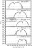Fig. B.1 Comparison of the energy distributions obtained from corresponding high and low resolution runs. The dashed lines indicate the mass resolution limits of the simulations, i.e. the mass of a single star particle.

To assess the influence of the numerical resolution on our results, we ran a set of simulations with the number of particles in the satellite system reduced by a factor of 10. This was done by taking the initial snapshot file of one of our high-resolution runs and randomly removing 90 percent of the satellite particles. Then the masses of the remaining particles increased by a factor of 10. In this way we obtain an equilibrium configuration of a satellite system with exactly the same properties as the high-resolution one.

In Fig. B.1 we show the resulting energy distributions, together with those of the corresponding high-resolution runs with the same initial conditions. The shapes of the distributions show no significant differences. The width of the corresponding distributions, ϵ_w, obtained by fitting Eq. (17) also differ by less than 10 percent. As could be expected, the low-resolution distribution does not reach as high an energy as the high-resolution one. However, the maximum energies do not differ by much, due to the steep slope in the outer tails of the distribution.

We also repeated one simulation run using a five times longer softening length for the star particles. For all quantities measured for this study the outcome changed by less than 1 percent. Especially the maximum energies reached by satellite particles differ only by 0.1 percent. This shows that our results are not affected by artificial heating by two-body encounters.

Appendix C: Other host galaxy potentials

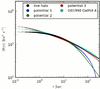Fig. C.1 Radial gravitational potential profiles of the four alternative host galaxy representation and for the N-body live host galaxy (black). The alternative models cover a variety of central and outer slopes allow testing of the influence of those on satellite tidal tails. The varying thickness of the profile lines reflects the nonspherical symmetry of the potentials.

To test the influence of the shape of the Milky Way-host potential, we performed a small number of test simulations with different rigid potentials representing the host galaxy. Four different models were applied: three of them (potentials 1–3) share the same parametrization of the baryonic disk and spheriod components. In three of the models the baryonic component of the Galaxy is modeled as a Miyamoto & Nagai (1975) disk with mass 10¹¹M_⊙, radial and vertical scale length of 6.5 and 0.26 kpc, respectively and a Hernquist (1990) bulge component of mass 3.4 × 10¹⁰M_⊙ and a scale length of 0.7 kpc. The dark halos are modeled with

• potential 1: a logarithmic potential$\mathrm{\Phi }\mathrm{\left(}\mathit{r}\mathrm{\right)}\mathrm{=}{\mathit{v}}_{\mathrm{h}}^{\mathrm{2}}\ln \mathrm{(}{\mathit{r}}^{\mathrm{2}}\mathrm{+}{\mathit{r}}_{\mathrm{h}}^{\mathrm{2}}\mathrm{)}$ with v_h = 128 km s^-1 and r_h = 12 kpc. This potential has already been often used by other studies to mimick a Milky Way (e.g. Johnston 1998; Helmi & White 2001);

• potential 2: a Plummer (1911) sphere with mass 6 × 10¹¹M_⊙ and scale radius 25.7 kpc;

• potential 3: an NFW sphere (Navarro et al. 1997) with central density 1.523 × 10⁶M_⊙kpc^-3 and scale radius 36 kpc.

All three potentials were chosen such that V_circ(8.5kpc) = 220 km s^-1 and V_esc(8.5kpc) = 550 km s^-1. As a fourth option we used the model potential number 4 of Dehnen & Binney (1998), which we implemented in Gadget-2 using a C++ routine prepared by Walter Dehnen and distributed with the NEMO Stellar Dynamics Toolbox (Teuben 1995).

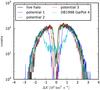Fig. C.2 Comparison of the energy distributions of the tidal tail particle stripped from identical satellite galaxies with identical initial phase space positions evolving in different host potentials.

Figure C.1 shows a comparison of the radial profiles of the four potentials with the radial profile of the live halo used in the main part of the simulations. All potentials have a steeper slope in the inner regions. The virtually flat part of the live potential is due to the gravitational softening becoming significant on these scales.

Figure C.2 plots the energy tidal tail distributions (cf. Fig. 6) obtained with the different host representations but otherwise identical initial conditions. While the distribution changes strongly in regions with small  | ΔE | , the tail of the distribution remains virtually unchanged. We thus conclude that the actual shape of the Galactic potential has no major influence on our results. The variations around the central minimum are most likely due to the different evolutions of the Roche radius of the satellite during its orbits thereby determining whether particles with low  | ΔE |  that stay near the satellite for longer periods are recaptured.

Appendix D: Initial conditions

References

All Tables

All Figures

	Fig. 1 Relation between the concentration parameter c of the dark halo and the total mass of the satellites. The black symbols show the applied values for the halo concentration parameter c for a given satellite mass Msat. The errorbars have a width of 0.5 to reflect that only integer numbers were used for c. The red line shows a power law with exponent 0.36.
In the text

Fig. 2 Aitoff projection of a simulation run about 200 Myr after perigalacticon. Green dots represent all satellite particles (only every 5th particle is plotted), while the MEPs are marked by red stars. The disk and bulge of the host galaxy are also shown as black mass-density contour lines. The median distance of the MEPs is  ~ 60 kpc, comparable to the Galactocentric distances of the observed HVSs. The MEPs are concentrated to confined area on the sky, in this case enclosed by a circle with angular radius 15°.

In the text

Fig. 3 Time series of the galactocentric RV-distance plane for two simulation runs. The time elapsed since perigalacticon, Δtperi, is shown in the upper left corner. Red stars represent the MEPs, green dots satellite particles, and dashed lines the local escape speed of the respective radius. Dotted lines mark lines of constant travel times corresponding to Δtperi. The eccentricity of the satellite orbit is given in the lower right corner of the rightmost panel. In the leftmost panels the mean distance of the MEPs is 60 kpc similar to the observed HVS population, which is shown in the right most panel in the upper row for comparison. None of the simulations were designed to reproduce the observed HVS population.

In the text

	Fig. 4 Snapshots of the satellite (small green dots) shortly before, during, and shortly after its pericentric passage. Red stars show the positions of those particles that will have the highest orbital energy at the end of the simulation. Blue triangles show those with the lowest energy.
In the text

Fig. 5 Energy gain with respect to Esat predicted by our simplified model ΔEmax compared to the maximum energy gain found in each simulation. The latter are by a factor of  ~0.45 (slope of the gray dotted lines) lower than the estimates, which is most likely due to oversimplification of the model. Phase-space sampling due to the limited particle number does not play a significant role as can be seen from the gray circles thAT mark the runs with 10 times lower resolution. Left: the estimated energy gain as obtained from our model. Right: the energy gain from our model corrected for an additional dependency on the angular momentum of the satellite. See text for a discussion.

In the text

Fig. 6 A histogram of the orbital energies of all particles that initially belonged to the satellite but became unbound to it in the course of the first orbit (tidal debris particles). The two peaks correspond to the two tidal arms torn out of the satellite. The central gap coincides with the orbital energy Esat of the remaining satellite system. The dashed red line shows the fitting function (Eq. (17)), which is used to characterize the distribution. The meaning of the fitting parameter ϵw, which is used to determine the width of the high energy peak, is also indicated.

In the text

Fig. 7 Upper panel: histograms of the energy differences ΔE = Ei − Esat of the tidal debris particles of all simulations used in this work overplotted. The distributions are plotted as functions of ΔE in units of the width of the high-energy peak ϵw. The histograms are also renormalized so that the high energy peak covers the same area. The lines are color-coded according to the initial angular momentum of the progenitor system (from red representing more radial orbits to blue for more circular orbits). Lower panel: the mean distribution obtained from the distribution plotted in the upper panel (solid black line). The standard deviation is also indicated with the thin gray lines. Overplotted in red is our fitting function using the parameters given in Eqs. (20) and ϵw = 1.

In the text

	Fig. 8 Relation between the maximum energy gain ΔEmax,sim and the width ϵw of the energy distribution of all tidal debris stars obtain via fitting Eq. (17). The gray dotted line has a slope of 1.5.
In the text

Fig. 9 The maximum ejection velocities at a galactocentric distance of 60 kpc as a function of initial satellite mass as computed from Eq. (23) assuming an initial orbital energy of the satellite Esat = 0 km2 s-2. The energy loss due to dynamical friction was computed using the empirical law (Eq. (14)) obtained from our simulations. The lower gray lines show the velocity of the satellite remnant at the same distance.

In the text

Fig. 10 Upper panel: mass ejected at unbound velocities during one satellite orbit as a function of initial progenitor mass. The satellite is assumed to have zero initial orbital energy, i.e. to be on a parabolic orbit. Different lines correspond to four different initial angular momenta of the satellite. The vertical dashed line indicates the mass of a single star particle in our simulations. Lower panel: mass fraction of an unbound intergalactic population originating in satellites with masses below Msat. The fraction were computed using satellite mass function based on the satellite luminosity function of Koposov et al. (2008). The mass function is also shown as a thin dashed line.

In the text

	Fig. B.1 Comparison of the energy distributions obtained from corresponding high and low resolution runs. The dashed lines indicate the mass resolution limits of the simulations, i.e. the mass of a single star particle.
In the text

	Fig. C.1 Radial gravitational potential profiles of the four alternative host galaxy representation and for the N-body live host galaxy (black). The alternative models cover a variety of central and outer slopes allow testing of the influence of those on satellite tidal tails. The varying thickness of the profile lines reflects the nonspherical symmetry of the potentials.
In the text

	Fig. C.2 Comparison of the energy distributions of the tidal tail particle stripped from identical satellite galaxies with identical initial phase space positions evolving in different host potentials.
In the text

References

- Abadi, M. G., Navarro, J. F., & Steinmetz, M. 2006, MNRAS, 365, 747 [NASA ADS] [CrossRef] [Google Scholar]
- Abadi, M. G., Navarro, J. F., & Steinmetz, M. 2009, ApJ, 691, L63 [NASA ADS] [CrossRef] [Google Scholar]
- Boylan-Kolchin, M., Besla, G., & Hernquist, L. 2011, MNRAS, 414, 1560 [NASA ADS] [CrossRef] [Google Scholar]
- Brooks, A. M., Governato, F., Quinn, T., Brook, C. B., & Wadsley, J. 2009, ApJ, 694, 396 [NASA ADS] [CrossRef] [Google Scholar]
- Brown, W. R., Geller, M. J., Kenyon, S. J., & Kurtz, M. J. 2005, ApJ, 622, L33 [NASA ADS] [CrossRef] [Google Scholar]
- Brown, W. R., Geller, M. J., Kenyon, S. J., & Kurtz, M. J. 2006a, ApJ, 640, L35 [NASA ADS] [CrossRef] [Google Scholar]
- Brown, W. R., Geller, M. J., Kenyon, S. J., & Kurtz, M. J. 2006b, ApJ, 647, 303 [NASA ADS] [CrossRef] [Google Scholar]
- Brown, W. R., Geller, M. J., Kenyon, S. J., Kurtz, M. J., & Bromley, B. C. 2007a, ApJ, 660, 311 [NASA ADS] [CrossRef] [Google Scholar]
- Brown, W. R., Geller, M. J., Kenyon, S. J., Kurtz, M. J., & Bromley, B. C. 2007b, ApJ, 671, 1708 [NASA ADS] [CrossRef] [Google Scholar]
- Brown, W. R., Geller, M. J., & Kenyon, S. J. 2009a, ApJ, 690, 1639 [NASA ADS] [CrossRef] [Google Scholar]
- Brown, W. R., Geller, M. J., Kenyon, S. J., & Bromley, B. C. 2009b, ApJ, 690, L69 [NASA ADS] [CrossRef] [Google Scholar]
- Bullock, J. S., & Johnston, K. V. 2005, ApJ, 635, 931 [NASA ADS] [CrossRef] [Google Scholar]
- Caldwell, N., Morrison, H., Kenyon, S. J., et al. 2010, AJ, 139, 372 [NASA ADS] [CrossRef] [Google Scholar]
- Chandrasekhar, S. 1943, ApJ, 97, 255 [NASA ADS] [CrossRef] [Google Scholar]
- Choi, J., Weinberg, M. D., & Katz, N. 2007, MNRAS, 381, 987 [NASA ADS] [CrossRef] [Google Scholar]
- Choi, J., Weinberg, M. D., & Katz, N. 2009, MNRAS, 400, 1247 [NASA ADS] [CrossRef] [Google Scholar]
- de Rijcke, S., Michielsen, D., Dejonghe, H., Zeilinger, W. W., & Hau, G. K. T. 2005, A&A, 438, 491 [NASA ADS] [CrossRef] [EDP Sciences] [Google Scholar]
- Dehnen, W., & Binney, J. 1998, MNRAS, 294, 429 [NASA ADS] [CrossRef] [Google Scholar]
- D’Onghia, E., Besla, G., Cox, T. J., & Hernquist, L. 2009, Nature, 460, 605 [NASA ADS] [CrossRef] [Google Scholar]
- D’Onghia, E., Vogelsberger, M., Faucher-Giguere, C.-A., & Hernquist, L. 2010, ApJ, 725, 353 [NASA ADS] [CrossRef] [Google Scholar]
- Edelmann, H., Napiwotzki, R., Heber, U., Christlieb, N., & Reimers, D. 2005, ApJ, 634, L181 [NASA ADS] [CrossRef] [Google Scholar]
- Fuentes, C. I., Stanek, K. Z., Gaudi, B. S., et al. 2006, ApJ, 636, L37 [NASA ADS] [CrossRef] [Google Scholar]
- Gan, J., Kang, X., van den Bosch, F. C., & Hou, J. 2010, MNRAS, 408, 2201 [NASA ADS] [CrossRef] [Google Scholar]
- Gnedin, O. Y., Gould, A., Miralda-Escudé, J., & Zentner, A. R. 2005, ApJ, 634, 344 [NASA ADS] [CrossRef] [Google Scholar]
- Guo, Q., White, S., Li, C., & Boylan-Kolchin, M. 2010, MNRAS, 404, 1111 [NASA ADS] [Google Scholar]
- Helmi, A., & White, S. D. M. 2001, MNRAS, 323; 529 [Google Scholar]
- Hernquist, L. 1990, ApJ, 356, 359 [NASA ADS] [CrossRef] [Google Scholar]
- Hernquist, L. 1993, ApJS, 86, 389 [NASA ADS] [CrossRef] [Google Scholar]
- Hills, J. G. 1988, Nature, 331, 687 [Google Scholar]
- Hirsch, H. A., Heber, U., O’Toole, S. J., & Bresolin, F. 2005, A&A, 444, L61 [NASA ADS] [CrossRef] [EDP Sciences] [Google Scholar]
- Johnston, K. V. 1998, ApJ, 495, 297 [NASA ADS] [CrossRef] [Google Scholar]
- Klypin, A., Zhao, H., & Somerville, R. S. 2002, ApJ, 573, 597 [Google Scholar]
- Koposov, S., Belokurov, V., Evans, N. W., et al. 2008, ApJ, 686, 279 [NASA ADS] [CrossRef] [Google Scholar]
- Kregel, M., van der Kruit, P. C., & de Grijs, R. 2002, MNRAS, 334, 646 [NASA ADS] [CrossRef] [Google Scholar]
- Law, D. R., Majewski, S. R., & Johnston, K. V. 2009, ApJ, 703, L67 [NASA ADS] [CrossRef] [Google Scholar]
- Levin, Y. 2006, ApJ, 653, 1203 [NASA ADS] [CrossRef] [Google Scholar]
- López-Morales, M., & Bonanos, A. Z. 2008, ApJ, 685, L47 [NASA ADS] [CrossRef] [Google Scholar]
- Lu, Y., Zhang, F., & Yu, Q. 2010, ApJ, 709, 1356 [NASA ADS] [CrossRef] [Google Scholar]
- McGaugh, S. S., Schombert, J. M., de Blok, W. J. G., & Zagursky, M. J. 2010, ApJ, 708, L14 [Google Scholar]
- Miyamoto, M., & Nagai, R. 1975, PASJ, 27, 533 [NASA ADS] [Google Scholar]
- Navarro, J. F., Frenk, C. S., & White, S. D. M. 1997, ApJ, 490, 493 [NASA ADS] [CrossRef] [Google Scholar]
- Perets, H. B., Hopman, C., & Alexander, T. 2007, ApJ, 656, 709 [NASA ADS] [CrossRef] [Google Scholar]
- Perets, H. B., Wu, X., Zhao, H. S., Famaey, B., et al. 2009, ApJ, 697, 2096 [NASA ADS] [CrossRef] [Google Scholar]
- Plummer, H. C. 1911, MNRAS, 71, 460 [CrossRef] [Google Scholar]
- Przybilla, N., Nieva, M. F., Tillich, A., et al. 2008, A&A, 488, L51 [NASA ADS] [CrossRef] [EDP Sciences] [Google Scholar]
- Przybilla, N., Tillich, A., Heber, U., & Scholz, R. 2010a, ApJ, 718, 37 [NASA ADS] [CrossRef] [Google Scholar]
- Przybilla, N., Tillich, A., Heber, U., & Scholz, R.-D. 2010b, ApJ, 718, 37 [NASA ADS] [CrossRef] [Google Scholar]
- Scannapieco, C., White, S. D. M., Springel, V., & Tissera, P. B. 2009, MNRAS, 396, 696 [NASA ADS] [CrossRef] [Google Scholar]
- Scannapieco, C., White, S., Springel, V., & Tissera, P. 2011, MNRAS, 417, 154 [NASA ADS] [CrossRef] [Google Scholar]
- Sesana, A., Madau, P., & Haardt, F. 2009, MNRAS, 392, L31 [NASA ADS] [Google Scholar]
- Smith, M. C., Ruchti, G. R., Helmi, A., et al. 2007, MNRAS, 379, 755 [NASA ADS] [CrossRef] [Google Scholar]
- Springel, V. 2005, MNRAS, 364, 1105 [NASA ADS] [CrossRef] [Google Scholar]
- Springel, V., & White, S. D. M. 1999, MNRAS, 307, 162 [NASA ADS] [CrossRef] [Google Scholar]
- Tamura, N., Hirashita, H., & Takeuchi, T. T. 2001, ApJ, 552, L113 [NASA ADS] [CrossRef] [Google Scholar]
- Taylor, J. E., & Babul, A. 2001, ApJ, 559, 716 [NASA ADS] [CrossRef] [Google Scholar]
- Teuben, P. 1995, in Astronomical Data Analysis Software and Systems IV, ed. R. A. Shaw, H. E. Payne, & J. J. E. Hayes, ASP Conf. Ser., 77, 398 [Google Scholar]
- Teyssier, M., Johnston, K. V., & Shara, M. M. 2009, ApJ, 707, L22 [NASA ADS] [CrossRef] [Google Scholar]
- Tillich, A., Przybilla, N., Scholz, R., & Heber, U. 2009, A&A, 507, L37 [NASA ADS] [CrossRef] [EDP Sciences] [Google Scholar]
- Tormen, G., Diaferio, A., & Syer, D. 1998, MNRAS, 299, 728 [Google Scholar]
- Warnick, K., Knebe, A., & Power, C. 2008, MNRAS, 385, 1859 [NASA ADS] [CrossRef] [Google Scholar]
- Xue, X. X., Rix, H. W., Zhao, G., et al. 2008, ApJ, 684, 1143 [NASA ADS] [CrossRef] [Google Scholar]
- Yu, Q., & Madau, P. 2007, MNRAS, 379, 1293 [NASA ADS] [CrossRef] [Google Scholar]
- Yu, Q., & Tremaine, S. 2003, ApJ, 599, 1129 [NASA ADS] [CrossRef] [Google Scholar]
- Zolotov, A., Willman, B., Brooks, A. M., et al. 2009, ApJ, 702, 1058 [NASA ADS] [CrossRef] [Google Scholar]