| Issue |
A&A
Volume 535, November 2011
|
|
|---|---|---|
| Article Number | A122 | |
| Number of page(s) | 11 | |
| Section | The Sun | |
| DOI | https://doi.org/10.1051/0004-6361/201117429 | |
| Published online | 23 November 2011 | |
Synthetic differential emission measure curves of prominence fine structures
II. The SoHO/SUMER prominence of 8 June 2004
1
Astronomical Institute, Academy of Sciences of the Czech
Republic, Fričova
298, 25165
Ondřejov, Czech
Republic
e-mail: This email address is being protected from spambots. You need JavaScript enabled to view it.
2
Royal Observatory of Belgium, 3 Av. Circulaire, 1180
Bruxelles,
Belgium
3
Max-Planck-Institut für Astrophysik, Karl-Schwarzschild-Strasse 1, 85740
Garching,
Germany
4
Institut d’Astrophysique Spatiale, Université Paris XI/CNRS,
91405
Orsay Cedex,
France
Received: 7 June 2011
Accepted: 13 September 2011
Abstract
Aims. This study is the first attempt to combine the prominence observations in Lyman, UV, and EUV lines with the determination of the prominence differential emission measure derived using two different techniques, one based on the inversion of the observed UV and EUV lines and the other employing 2D non-LTE prominence fine-structure modeling of the Lyman spectra.
Methods. We use a trial-and-error method to derive the 2D multi-thread prominence fine-structure model producing synthetic Lyman spectra in good agreement with the observations. We then employ a numerical method to perform the forward determination of the DEM from 2D multi-thread models and compare the synthetic DEM curves with those derived from observations using inversion techniques.
Results. A set of available observations of the June 8, 2004 prominence allows us to determine the range of input parameters, which contains models producing synthetic Lyman spectra in good agreement with the observations. We select three models, which represent this parametric-space area well and compute the synthetic DEM curves for multi-thread realizations of these models. The synthetic DEM curves of selected models are in good agreement with the DEM curves derived from the observations.
Conclusions. We show that the evaluation of the prominence fine-structure DEM complements the analysis of the prominence hydrogen Lyman spectra and that its combination with the detailed radiative-transfer modeling of prominence fine structures provides a useful tool for investigating the prominence temperature structure from the cool core to the prominence-corona transition region.
Key words: Sun: filaments, prominences / techniques: spectroscopic / methods: data analysis / methods: numerical
© ESO, 2011
1. Introduction
Solar prominences are highly-structured objects located in the solar corona that are considerably denser and cooler than their surrounding environment. The temperature of the prominence plasma, suspended in predominantly horizontal magnetic fields, varies from the cool core with typical values between 6000 and 8000 K towards coronal values on the order of 1 million K (see e.g. Tandberg-Hanssen 1995). The region where the temperature rises from prominence to coronal values is usually called the prominence-corona transition region (PCTR). The geometrical extension of the PCTR and subsequently the gradient of the temperature can vary considerably depending on the orientation of the magnetic field with respect to the direction of the geometrical structure. In general, in the direction across the magnetic field lines the PCTR can be extremely narrow (with very steep temperature gradients), while in the direction along the magnetic field the PCTR can be much more extended. These properties of the PCTR are attributed to the considerable suppression of the thermal conductivity in the direction across the magnetic field. The UV and EUV spectral lines emitted in the PCTR plasma provide useful tools for the understanding of the temperature structure and the thermodynamical properties of these regions and therefore have been the subject of many past (Orrall & Schmahl 1976; Engvold 1988) and recent (Patsourakos & Vial 2002) prominence observations from space. A summary of the studies concerning these PCTR UV and EUV spectral lines can be found in the review by Labrosse et al. (2010).
To obtain some information about the plasma in these transition regions, one can use the differential emission measure (DEM), which provides information about the plasma distribution as a function of the temperature along a given line of sight (LOS). However, the DEM itself does not allow the determination of the spatial distribution of the plasma along the given LOS. Only in the simplest cases of 1D slab configurations can one use the derived DEM(T) curves to determine the temperature structure of the PCTR. The DEM curve can be derived from a set of observed UV and EUV lines, assuming that the lines are optically thin (see e.g. Wiik et al. 1993; Cirigliano et al. 2004; Parenti & Vial 2007), by using inversion techniques such as those available in the CHIANTI software (see e.g. Parenti & Vial 2007; Phillips et al. 2008).
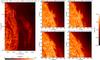 |
Fig. 1 Images obtained by the SoHO/EIT in the He ii 304 Å line. The position of the SUMER slit is marked in all panels by the white vertical bar in all panels, although the SoHO/SUMER observations were done only between June 7, 23:35 UT and June 8, 5:54 UT. The scale-scale bars give the DN-to-pixel ratio in the logarithmic scale. |
The prominence DEM can be also obtained by theoretical modeling, e.g., by employing 1D magnetohydrostatic (MHS) slab models with a given PCTR structure (Anzer & Heinzel 1999, 2000, 2008) or by assuming an ensemble of horizontal magnetic flux tubes (Chiuderi Drago et al. 1992). A more realistic method for obtaining synthetic DEM curves for solar prominences was used by Gunár et al. (2011), hereafter referred to as Paper I. In this paper, we employed 2D models of prominence fine structures developed by Heinzel & Anzer (2001) in configurations with randomly distributed threads (used for prominence modeling by Gunár et al. 2007b, 2008, 2010). In Paper I, we presented a numerical method for the derivation of the synthetic DEM curves from a specific temperature and density structure provided by 2D multi-thread models, which can produce synthetic Lyman spectra that are in good agreement with the observations (Gunár et al. 2007b, 2008, 2010) and showed that these synthetic DEM curves are in agreement with the DEM curves derived from the observations.
In the present study, we employ 2D multi-thread prominence fine-structure models and use a trial-and-error method to derive prominence models producing synthetic Lyman spectra consistent with prominence observations obtained by SoHO/SUMER on June 8, 2004. Owing to the nature of the available set of observations (non-reversed low intensity Lyman line profiles and nonavailability of the Lyman-α and Hα line observations), we are unable to derive a unique set of model input parameters but instead we broadly specify a parametric space area containing models that produce synthetic Lyman spectra in agreement with the observed ones. We select three models characterizing this parametric space area and derive the synthetic DEM curves for these prominence fine-structure models using the numerical method from Paper I. We compare the obtained synthetic DEM curves with the DEM curves derived from observed UV and EUV spectra of the June 8, 2004 prominence. The synthetic DEM curves of selected 2D multi-thread prominence fine-structure models are, in the temperature range covered by models, in very good agreement with the observed ones.
The paper is organized as follows. Sections 2 and 3 give details about the Lyman lines observations, and the UV and EUV line observations and the observed DEM determination, respectively. In Sect. 4, we give a brief description of our 2D prominence fine-structure models. Section 5 presents the selected 2D multi-thread models and their synthetic Lyman spectra. Section 6 presents the synthetic DEM curves of selected models and Sects. 7 and 8 provide the discussion and our conclusions.
2. Observational data
The prominence observational data used in this study were obtained during the 13th MEDOC campaign by SUMER (Solar Ultraviolet Measurements of Emitted Radiation) UV-spectrograph (Wilhelm et al. 1995) onboard SoHO (Solar and Heliospheric Observatory). The observed prominence was located at the NW limb and crossed the limb for several days, as can be seen in the sequence of SoHO/EIT (Extreme-ultraviolet Imaging Telescope, Delaboudinière et al. 1995) 304 channel images shown in Fig. 1. This prominence was not associated with any active region and only partially connected to the erupting prominence located further to the west. It remained low-lying and stable for several consecutive days and disappeared several hours after the SoHO/SUMER observing program was completed. No signs of activation can be found in the available observed data, which suggests that this prominence disappeared beyond the solar limb due to the solar rotation. The relatively stable nature of the observed prominence allows us to consider it as a quiescent prominence, although significant plasma motions and temporal variations might be present because of its closeness to an eruptive prominence. The SoHO/SUMER slit (n. 4, 1″ × 120″) was centered at X = 890′′, Y = 420′′ and intersected the central part of the prominence composed of many fine structures. The SoHO/SUMER observing program run between June 7, 23:35 UT and June 8, 5:54 UT and the observations were performed by running one of the reference spectrum observing programs (lem_ref_a_prom2003), which scans the full spectrum of detector A (from about 800 to 1600 Å) using 40 Å windows in successive exposures of 370 s each. Due to the long time-period needed to scan the full spectrum, the hydrogen Lyman lines cannot be observed co-temporally and the Lyman-β and Lyman-δ line observations are separated by a time difference of about 30 min.
The observed spectra were reduced and calibrated using standard SolarSoft procedures for the SUMER data, which include corrections for geometrical distortion and flat-fielding. The data in each spectral window were calibrated in wavelength as described in Parenti et al. (2004), and in intensity using the standard Radiometry procedure. The spectral line fluxes used for the analysis were obtained by a multi-Gaussian line-fitting (as described in Parenti et al. 2005) and are given in Table 1. Most of the lines used in this work had already been identified by Parenti et al. (2005) as the most suitable for the DEM inversion due to their relatively high signal-to-noise ratios and marginal contamination by blends, which are either absent or easy to eliminate using the multi-Gaussian fitting.
List of lines used for derivation of the observed DEM.
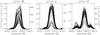 |
Fig. 2 The observed Lyman-β to Lyman-δ lines obtained by SoHO/SUMER on June 8, 2004. |
During these observations, detector A already showed a gain loss in its central part, which involved seven detector rows (W. Curdt, pers. comm.). This degraded part of the detector was located within the central part of the observed prominence and caused the signal from the degraded rows, to overflow into adjacent rows where it was added to the actual signal of these rows. The determination of the DEM requires the use of average line emission over as many pixels as possible in order to maximize the signal-to-noise ratio of these lines and thus the accuracy of the inversion method. Since the signal from the degraded part of the detector was not lost but added to adjacent rows of the SUMER slit, we were able to use the average emission from the whole portion of the slit (from pixel 20 to 70) covering the prominence for the DEM determination. On the other hand, the deteriorated rows together with the adjacent rows affected by the signal overflow, had to be excluded from the analysis of the Lyman lines because individual observed line profiles were affected and only 36 positions along the SUMER slit were used (see Fig. 2). The integrated intensities of these observed Lyman lines (in erg s-1 cm-2 sr-1) range from 1232 to 6535 for Lyman-β, from 157 to 1503 for Lyman-γ, and from 164 to 535 for Lyman-δ.
3. DEM derived from observations
The DEM is a widely studied plasma parameter, which, assuming a monotonic temperature
variation along a given LOS (h), is usually defined as (see e.g. Mariska 1992; Phillips
et al. 2008) 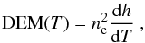 (1)where ne is the
electron density at the LOS position h with a given temperature
T. The DEM is related to the integrated intensity I of
an optically thin line through the equation
(1)where ne is the
electron density at the LOS position h with a given temperature
T. The DEM is related to the integrated intensity I of
an optically thin line through the equation 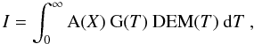 (2)where A(X) is
the element abundance with respect to hydrogen and G(T) is
the contribution function for a given spectral line, which contains the atomic information
of the transition involved.
(2)where A(X) is
the element abundance with respect to hydrogen and G(T) is
the contribution function for a given spectral line, which contains the atomic information
of the transition involved.
We derived the DEM curve for the June 8, 2004 prominence by applying a version of the maximum entropy method described in Monsignori Fossi & Landini (1991) implemented by del Zanna (1999) on the set of observed UV and EUV spectral lines listed in Table 1. The theoretical emissivities were calculated using the CHIANTI atomic database, using the ionization equilibrium data of Mazzotta et al. (1998), photospheric element abundances (Grevesse et al. 2007), and a constant pressure in terms of neT of 4 × 1013 cm-3 K, which corresponds to a gas pressure of about 0.01 dyn cm-2. The best-fit solution is obtained by minimizing the difference between the theoretical and measured intensities. This ratio is, for most of our lines, within 20% and it can reach about 40% at worst case. This is a reasonable solution considering that the atomic physics uncertainties themselves can reach up to the 30% (Landi & Klimchuk 2010). The derived DEM curve is shown in Fig. 3.
The high-temperature part of this DEM curve is affected by the contamination of lines used for DEM derivation by the foreground and background coronal emission (see e.g. Labrosse et al. 2010). Thus for the June 8 prominence, the most reliable part of the derived DEM curve is the low-temperature portion lying below 105 K, where the value of the minimum temperature of the DEM curve is constrained by several C ii and N ii lines. The set of available observations of the studied prominence does not allow the use of cooler lines such as those used by Parenti & Vial (2007) due to their very low signal-to-noise ratios. Parenti & Vial (2007) used the SoHO/SUMER spectral atlas obtained by Parenti et al. (2004, 2005) to derive the DEM for a quiescent prominence observed in 1999, where cooler lines such as Si ii were present.
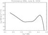 |
Fig. 3 The DEM curve of the June 8, 2004 prominence as a function of the temperature drawn in the log-log scale. |
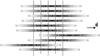 |
Fig. 4 Vertical projection of a randomly generated multi-thread configuration with randomly shifted threads drawn to proper geometrical scale. The orientation of the magnetic field is indicated by an arrow. |
4. Prominence fine-structure models
To obtain synthetic Lyman-line spectra, we employ 2D models of prominence fine structures
in multi-thread configurations. These 2D models that depict fine structures of prominences
in the form of vertically infinite two-dimensional threads embedded in a horizontal magnetic
field, were developed by Heinzel & Anzer (2001).
These threads are uniform in the vertical direction and the variations take place only in
the horizontal plane parallel to the solar surface. The 2D threads are in a MHS equilibrium
of the Kippenhahn-Schlüter type (Kippenhahn & Schlüter
1957) that was generalized to 2D by Heinzel &
Anzer (2001) and their temperature structure is specified empirically to encompass
both the central cool part and also the PCTR (see Anzer &
Heinzel 1999). The PCTR exhibits two distinct forms with a steep temperature
gradient in the direction across the magnetic field lines within a narrow PCTR layer and
much more extended part in the direction along the field where the temperature gradually
rises from the cool core towards the thread boundaries. This approach is used because the
heat conduction is much lower in the direction across the magnetic field lines than along
the field. This temperature structure is characterized by an analytic formula ![Mathematical equation: \begin{equation} \label{T} T(m,y)=T_{{\rm cen}}(y)+[T_{{\rm tr}}-T_{{\rm cen}}(y)]\left\{1-4\frac{m}{M(y)}\left[1-\frac{m} {M(y)}\right]\right\}^{\gamma_{1}} , \end{equation}](/articles/aa/full_html/2011/11/aa17429-11/aa17429-11-eq26.png) (3)where Tcen is given
by
(3)where Tcen is given
by 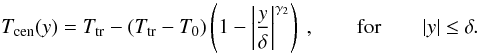 (4)Here, the column-mass scale m
is parallel to the x-direction with a simple relation through the plasma
density, M(y) represents the column mass integrated in the
x-direction, and 2δ is the width of the thread
perpendicular to the field lines. The temperature T0 represents
the minimum temperature at the center of the thread, Ttr is the
boundary transition-region (tr) temperature at the thread boundaries, and the exponents
γ1 and γ2 describe the temperature
gradients within the PCTR, where γ2 represents the steep
temperature gradient in the direction across the magnetic field lines and
γ1 the more gentle gradient along the field. These four
parameters, together with Bx(0) representing
the magnetic field strength in the middle of the thread, M0
giving the maximum column density, and ptr, which is the value
of the gas pressure at the thread boundaries, form the set of input parameters describing
the MHS structure of the 2D models. The geometrical dimensions of the 2D thread are
determined in the following way: the length of the thread in the
x-direction (along the magnetic field lines) is the result of the MHS
equilibrium and is unique to each set of model input parameters, while the width of the
thread in the y-direction (across the field lines) is chosen arbitrarily.
We take the value of the thread width to be 1000 km, which is consistent with our previous
prominence modeling and approximately represents the spatial resolution of SoHO/SUMER.
However, observations of the prominence and filament fine structures in the hydrogen
Hα line, such as those by Lin et al.
(2005), indicate that the widths of these fine structures can be as small as
100 km.
(4)Here, the column-mass scale m
is parallel to the x-direction with a simple relation through the plasma
density, M(y) represents the column mass integrated in the
x-direction, and 2δ is the width of the thread
perpendicular to the field lines. The temperature T0 represents
the minimum temperature at the center of the thread, Ttr is the
boundary transition-region (tr) temperature at the thread boundaries, and the exponents
γ1 and γ2 describe the temperature
gradients within the PCTR, where γ2 represents the steep
temperature gradient in the direction across the magnetic field lines and
γ1 the more gentle gradient along the field. These four
parameters, together with Bx(0) representing
the magnetic field strength in the middle of the thread, M0
giving the maximum column density, and ptr, which is the value
of the gas pressure at the thread boundaries, form the set of input parameters describing
the MHS structure of the 2D models. The geometrical dimensions of the 2D thread are
determined in the following way: the length of the thread in the
x-direction (along the magnetic field lines) is the result of the MHS
equilibrium and is unique to each set of model input parameters, while the width of the
thread in the y-direction (across the field lines) is chosen arbitrarily.
We take the value of the thread width to be 1000 km, which is consistent with our previous
prominence modeling and approximately represents the spatial resolution of SoHO/SUMER.
However, observations of the prominence and filament fine structures in the hydrogen
Hα line, such as those by Lin et al.
(2005), indicate that the widths of these fine structures can be as small as
100 km.
To determine the synthetic hydrogen spectra emerging from 2D fine-structure threads, we solve the 2D multi-level non-LTE (i.e. departure from local thermodynamic equilibrium) radiative transfer problem in these fine structures. The details of the method are given in Heinzel & Anzer (2001) and Heinzel et al. (2005). The obtained synthetic spectra can be compared with the observed prominence spectra in order to derive the parameters of the prominence fine structures (see Gunár et al. 2007b, 2008, 2010). By solving the non-LTE radiative transfer within 2D threads, we also determine the proper ionization degree of the hydrogen plasma and thus obtain the true variation of the electron density within these 2D prominence fine-structure threads, which is needed for consistent solution of the MHS equilibria. The ionization degree is determined iteratively, as described in Heinzel & Anzer (2003).
In the present study, we use multi-thread configurations of the 2D prominence fine-structure models, which can produce synthetic Lyman spectra in better agreement with observations than single-thread models (Gunár et al. 2007b). The individual threads of these multi-thread models are randomly shifted with respect to the foremost thread (see Fig. 4) to resemble the non-uniformity of the prominence fine structures. The maximum shift of any thread is equal to half the length of each thread. We use multi-thread models consisting of N identical threads without any mutual radiative interaction between individual threads (all parameters are identical for each thread resulting in identical temperature and electron density structures for all threads). We also randomly assign a LOS velocity to each thread, which allows us to obtain asymmetrical Lyman line profiles in accordance with the observations (Gunár et al. 2008).
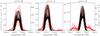 |
Fig. 5 Comparison of observed Lyman-β to Lyman-δ lines (red dashed lines) with synthetic lines (black solid lines) for a randomly generated realization of Model_dem with ten identical threads. |
5. Synthetic Lyman line spectra
All the observed Lyman lines exhibit non-reversed profiles (i.e. without any central reversal) with relatively low intensities. This indicates that the column mass along the LOS is small (see the discussion about the model input parameters in Sect. 4.2 of Berlicki et al. 2011). Thus, we started with the configuration based upon the so-called Model2 as an initial guess and proceeded by the trial-and-error method to determine a model producing synthetic Lyman spectra in agreement with the observations. Model2 was studied by Berlicki et al. (2011) and used in Paper I to analyze the synthetic DEM curves of prominence fine structures.
We employed the multi-thread configuration of the 2D prominence fine-structure model with ten identical threads and LOS velocities ranging between –10 and 10 km s-1; and by making profile-to-profile comparisons of the synthetic and observed Lyman lines, we derived a set of input parameters defining a 2D model in good agreement with observations. In the present study, we refer to this model as the Model_dem, and we provide details of its input parameters and comment on its uniqueness in the following sections.
To determine suitable models, we used multi-thread configurations with ten threads, which is consistent with the number of threads used by Gunár et al. (2007b, 2008, 2010) but differs from the modeling of Berlicki et al. (2011), who used 40 threads to obtain agreement with the observed Hα line spectra. However, for the prominence studied in the present work, no simultaneous Hα observations, either imaging or spectral, do exist. Therefore, we were unable to reliably estimate the number of threads because the number of threads in our 2D multi-thread models have little effect on the shape of the Lyman line profiles. This is due to the high optical thickness of even the higher members of the Lyman series at the center of the lines. A larger number of threads affects only the widths of the synthetic Lyman lines, which become slightly wider. However, this effect is coupled with additional changes in the line widths caused by the random shifts of the threads with respect to the foremost one and with the effect of the stochastic LOS velocities, which also slightly increase the widths of the line profiles with increasing LOS velocity values. Thus, in the absence of some additional constraint such as Hα observations, and in accordance with the latter results of the DEM analysis, we used ten threads as a standard number of threads in the multi-thread models for the present investigation. The observed prominence crossed the solar limb over a period of several consecutive days (Fig. 1), which implies that we observed this prominence more-or-less along its spine. This an orientation of the LOS would result in its crossing a larger number of fine structures, which is in agreement with multi-thread models composed of ten or more threads. We also used as a standard the LOS velocities from interval of –10 to 10 km s-1. Such LOS velocities are expected to prevail within quiescent prominences and can produce synthetic Lyman line profiles with asymmetries comparable to the observations (Gunár et al. 2008). In the prominence studied here, we could expect even larger velocities. However, without sufficiently large data sets of observed Lyman lines and some proper statistical analysis (such as in Gunár et al. 2010) we were unable to determine the correct values of the LOS velocities in this prominence. Unfortunately, such a large set of quasi-co-temporal observations of the Lyman lines cannot be achieved with SoHO/SUMER in combination with the long-lasting observations that one needs for the determination of the observed DEM curve of this prominence. The determination of the LOS velocities is only of marginal interest to the present study because these do not affect the DEM calculations.
5.1. Description of Model_DEM
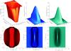 |
Fig. 6 Temperature, electron density, and gas pressure variations of the Model_dem. Note that these plots are not drawn to the proper geometrical scale. |
List of input parameters of selected models.
The multi-thread configuration of Model_dem with tenidentical threads and both random shifts and random LOS velocities in the interval between –10 to 10 km s-1, gives a reasonably good agreement between the synthetic and the observed Lyman line profiles. We compare the synthetic with observed Lyman-β to Lyman-δ lines for a randomly generated configuration in Fig. 5. In red dashed lines, we plot the observed Lyman line profiles at 36 positions along the SUMER slit. Black solid lines represent the synthetic profiles at 83 positions along the foremost thread. The synthetic Lyman lines above Lyman-δ obtained by our 2D models have intensities that are inconsistent with the observations. However, this is caused by the approximation of a portion of incident radiation adopted by our models and we will address this issue in the future. For this reason, we do not use lines higher than Lyman-δ in the present investigation.
The input parameters of the Model_dem are listed in Table 2. The values of the minimum central temperature T0, the magnetic field strength in the middle of the thread Bx(0), and the maximum column density along the length of the thread M0 are in the range of values expected for the conditions of the quiescent prominences (see review by Labrosse et al. 2010). The boundary temperature Ttr was chosen to be equal to 105 K, which is well above the temperature where hydrogen is fully ionized. The value of the boundary gas pressure ptr is relatively low but still comparable with the Model1 used in our previous modeling. The central gas pressure pcen is not an input parameter but is instead determined by the MHS equilibrium together with the geometrical extension of the thread in the direction along the magnetic field (in the x-direction), which is equal to 25 000 km. In Fig. 6, we show the temperature, electron density, and gas pressure variations of the Model_dem. We note that these plots are not drawn to the proper geometrical scale: the 2D threads are actually far more extended in the x-direction (along the field lines).
5.2. Sensitivity and uniqueness of the model
The 2D prominence fine-structure models are rather sensitive to the choice of most of the input parameters, even if we consider low-mass, low-pressure models such as the Model_dem. However, the available observations of the prominence studied in this work, consist only of Lyman lines excluding Lyman-α and these lines are non-reversed and have low intensities. Such a set of observations does not place sufficient constraints on the modeling and thus we were unable to determine a truly unique model for this prominence. Instead, we define an area in the parametric space of the model input parameters, which contains 2D models producing synthetic Lyman spectra similar to that of the Model_dem.
In the following text, we discuss the role of individual input parameters and the effects of their variations on the synthetic Lyman lines. We note that these discussions are valid only for models producing low-intensity non-reversed Lyman lines obtained along a LOS oriented either along or across the magnetic field lines.
A change of the value of the central minimum temperature T0 has no significant effect on the synthetic Lyman line profiles of the low-mass low-pressure models, although it has a strong influence on the synthetic line profiles of more massive models producing reversed profiles when observed across the magnetic field lines. Thus, in the absence of Hα line observations (Hα is formed in the cool core of the prominence fine structures and is therefore sensitive to the choice of T0) we were unable to determine a precise value of the central temperature. However, the value of T0 does not affect the prominence DEM and so its determination is not critical for the goals of this study.
We now concentrate on the input parameters that have a significant effect on the synthetic spectra, the column mass at the center of the thread M0 and the boundary gas pressure ptr. The variation in each of these parameters, which is of the order of 20% from Model_dem values, leads to synthetic profiles that are systematically either more (for higher values) or less (for lower values) intense than the observed profiles. This reveals the high sensitivity of our 2D prominence fine-structure models and suggests that we might be able to determine a unique model. However, with low-intensity, non-reversed observed Lyman-line profiles (moreover without the Lyman-α line) and in the absence of an observed Hα line, we are not able to uniquely determine the amount of mass in the studied prominence. And because the combination of lower M0 and higher ptr, or vice versa, can lead to models producing similar synthetic Lyman lines than those of the Model_dem this model is not a unique solution of our modeling of the June 8, 2004 prominence. By increasing M0 and decreasing ptr, we can find a model producing synthetic Lyman spectra in agreement with observations with values of M0 = 4 × 10⁻⁵ g cm-2 and ptr = 0.007 dyn cm-2. This model has a very low value of the boundary gas pressure and a rather large geometrical extension along the magnetic field determined by MHS equilibrium, equal to 35 000 km. We refer to this model as Model_dem_var1 (see Table 2). However, an additional increase of M0 to for instance 5 × 10⁻⁵ g cm-2 leads to models producing self-reversed Lyman line profiles, even when ptr is set to extremely low values of 0.003 dyn cm-2. Moreover, these models have very large geometrical extensions along the magnetic field lines of more than 50 000 km. In the opposite direction, by decreasing M0 and increasing ptr we can find a suitable model with values of M0 = 2 × 10⁻⁵ g cm-2 and ptr = 0.015 dyn cm-2, which we call Model_dem_var2 (see Table 2), and a geometrical extension in the x-direction of 15 000 km. An additional decrease of M0 to 0.5 × 10⁻⁵ g cm-2 and increase of ptr to 0.03 dyn cm-2 also leads to a model producing synthetic spectra in reasonable agreement with the observations, although such model has a very short geometrical extension of less then 3000 km and a central gas pressure lower then 0.035 dyn cm-2, which corresponds to an almost isobaric model with an extremely shallow dip.
The magnetic field strength Bx(0) affects, together with the column mass and boundary gas pressure, the shape of the magnetic produced by the MHS equilibrium. All models discussed above have the value of Bx(0) = 5 Gauss. The variation of this value between 4 and 6 Gauss in addition to the corresponding decrease (for lower Bx(0)) or increase (for higher Bx(0)) in the column mass leads to models with similar synthetic Lyman spectra as those of the selected set of models. These values correspond to the values expected under the conditions of quiescent solar prominences. However, the present set of observational constraints does not allow a more accurate determination of the magnetic field strength.
The last two input parameters of our 2D prominence fine-structure models are the exponents γ1 and γ2 defining the temperature gradients in the PCTR, where γ2 describes the steep gradient of the temperature across the magnetic field lines and γ1 describes the gradual temperature rise along the field. For all variations of the Model_dem discussed above, these exponents are set to values of γ1 = 10 and γ2 = 60. A change of the value of γ2 to 30 does not have any effect on the synthetic Lyman line profiles because these are not formed, in less massive models, in the very narrow PCTR layer extending across the magnetic field but deeper in the thread. On the other hand, a change of the value of γ1 to 5 leads to suitable models with approximately 30% to 50% lower values of M0 for a given value of ptr. Thus, an equivalent model to the Model_dem producing similar synthetic Lyman spectra has M0 = 2 × 10⁻⁵ g cm-2 and the same ptr = 0.010 dyn cm-2 as the Model_dem.
The parametric space area that includes models producing synthetic Lyman line profiles in agreement with the observed ones thus lies within the following range of the model input parameters: the magnetic field strength Bx(0) between 4 and 6 Gauss and the column mass in the center of the thread M0 between 1 and 4 × 10⁻⁵ g cm-2, in correspondence with the boundary gas pressure ptr between 0.02 and 0.007 dyn cm-2, depending on the exponent γ1. The minimum temperature at the center of the thread T0 cannot be determined precisely because of a lack of the Hα observations but can have values in the range of 6000 to 8000 K, which can be expected in the quiescent solar prominences (see e.g. Tandberg-Hanssen 1995).
6. Calculation of synthetic DEM curves
To derive the synthetic DEM curve for 2D prominence fine-structure models, we used a
forward method described in Paper I, which calculates the DEM values from the temperature
and electron density variations provided by the 2D models. To achieve this, the temperature
range is divided into a number of equidistant temperature bins
Ti (where
Ti goes from T0
to Ttr) with bin-width
ΔTi for a given LOS. Since the temperature
profile of 2D models in both single-thread and multi-thread configurations is not a
monotonic function along any given LOS (see Fig. 6),
multiple regions with the same temperature along a given LOS contribute to the DEM in the
given temperature bin. For a sufficiently small temperature bin-width
ΔTi, we then obtain the following formula
for DEM(Ti) 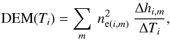 (5)where
Δhi,m is the geometrical length of a LOS
segment corresponding to the temperature bin
⟨Ti , Ti + ΔTi⟩
of the region m, and ne(i,m)
represents the mean value of the electron density at the LOS segment
Δhi,m. We sum over all regions with the
same temperature Ti along a given LOS (see also
Frazin et al. 2005). This method of forward DEM
computation does not depend on the choice of the temperature bin-width
ΔTi as long as this is sufficiently small.
It also does not suffer from the effects of averaging the electron density over extended
heterogeneous areas (see Judge 2000) because we use
the average values only over small LOS segments
Δhi,m.
(5)where
Δhi,m is the geometrical length of a LOS
segment corresponding to the temperature bin
⟨Ti , Ti + ΔTi⟩
of the region m, and ne(i,m)
represents the mean value of the electron density at the LOS segment
Δhi,m. We sum over all regions with the
same temperature Ti along a given LOS (see also
Frazin et al. 2005). This method of forward DEM
computation does not depend on the choice of the temperature bin-width
ΔTi as long as this is sufficiently small.
It also does not suffer from the effects of averaging the electron density over extended
heterogeneous areas (see Judge 2000) because we use
the average values only over small LOS segments
Δhi,m.
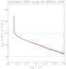 |
Fig. 7 Synthetic DEM curve (solid black line) of one randomly generated realization of the multi-thread Model_dem with 10 threads. The red dash-dotted line represents the DEM derived from the observations of the June 8, 2004 prominence. The blue dashed-line rectangle shows the segment used to display the DEM curves in the following plots. |
For a specific LOS, the resulting synthetic DEM curve can exhibit rather large variations depending on the local values of the temperature and electron density along this LOS. However, the observed DEM curves can be derived only for sufficiently large parts of the prominence, typically wider than ten thousand km, because of the low signal-to-noise ratio of PCTR spectral lines. This implies that the observed DEM should by averaged over large fractions of the entire prominence. Moreover, the inversion techniques used to derive the DEM curves from the observed PCTR spectral lines inherently smooth out any large local variations in the DEM. Hence, only the synthetic DEM curves averaged over large portions of the 2D threads can be compared with the DEM curves derived from the observations. To accurately describe the temperature distribution of the 2D model with its steep temperature gradients, it is important to derive the synthetic DEM for a large number of lines of sight (typically several thousands) spanning the given portion of the 2D model. The geometrical distance between individual lines of sight should be comparable to the smallest lengths Δhi,m of any given LOS segment corresponding to the temperature bin ⟨Ti , Ti + ΔTi⟩. Thus, the derived averaged synthetic DEM curves are smooth and without any large variations and can be easily compared with the DEM curves derived from the observations.
6.1. Comparison of observed and synthetic DEM curves
In this study, we have derived the synthetic DEM for 2D multi-thread models with a LOS perpendicular to the magnetic field lines. To analyze the synthetic DEM curves, we average the synthetic DEM over the whole length of the foremost thread of the multi-thread models, which is different for each model used. We omit the analysis of the synthetic DEM curves obtained with a LOS oriented along the field lines because the low-mass models produce similar synthetic Lyman line profiles in both directions (see Berlicki et al. 2011) and because we are unable to distinguish the LOS orientation owing to the lack of additional observational constraints, mainly for the Hα line profiles. Therefore, we focus on the probability of the LOS orientation, which is parallel to the magnetic field lines, being significantly lower than the across-the-field orientation, which is caused by the geometrical shape of the threads with lengths of several 10 000 km and widths of only 1000 km.
As in our previous investigations, we considered here only those parts of the PCTR that lie below 100 000 K, which is the boundary temperature of our models. This temperature lies well above the temperatures where hydrogen is fully ionised and all Lyman lines are formed. The minimum temperature of all our models amounts to 8000 K at the center of each thread. However, the determination of the DEM from observations does not produce reliable results at such low temperatures. For this reason, we compared the observed and synthetic DEM curves only in the range between log T = 4.3 K (approximately 20 000 K) and 100 000 K.
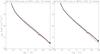 |
Fig. 8 Synthetic DEM curves of the Model_dem in multi-thread configuration with 10 (left panel) and 15 threads (right panel). Gray solid lines represent 100 random realizations of the multi-thread model and the black solid line gives the average of these 100 realizations. Red dash-dotted line represents the observed DEM curve. |
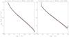 |
Fig. 9 Same as in Fig. 8 but here we plot synthetic DEM curves for 10-thread realizations of the Model_dem_var1 on the left and Model_dem_var2 on the right. |
Figure 7 shows the whole synthetic DEM curve (solid black line) of a randomly generated realization of the multi-thread Model_dem with ten stochastically arranged threads in comparison with the DEM curve derived from the observations of the 8 June 2004 prominence (red dash-dotted line). The synthetic DEM curve is averaged over the length of the foremost thread, which for Model_dem equals 25 000 km. The x and y-axis in this plot cover the same ranges as those in Paper I. The blue dashed-line rectangle shows the segment used to display the DEM curves in the following plots. Figure 8 shows a detailed comparison between the synthetic DEM curves of the Model_dem in the multi-thread configuration with 10 (left panel) and 15 threads (right panel), with the DEM curve derived from the observations drawn as red dash-dotted line. Gray solid lines indicate the 100 random realizations of the multi-thread model and the black solid line the average of these 100 realizations. All synthetic DEM curves represent the averaged DEM over the length of the foremost thread of the given multi-thread configuration. We note that a small dip in the synthetic DEM curves at about log T = 4.7 is an artefact of the numerical DEM derivation. The agreement in the slope of the DEM curve between the observed and synthetic DEM is very good for all multi-thread realizations. The absolute value of the DEM derived from the observations corresponds to a multi-thread model whose number of threads range between 10 and 15. We also show, in Fig. 9, the synthetic DEM curves of models Model_dem_var1 and Model_dem_var2, both with ten threads in random multi-thread configurations. These results are similar to those of the Model_dem, although the slope of the DEM curves is slightly different.
7. Discussion
This study is the first attempt to combine the prominence observations in Lyman, UV, and EUV PCTR lines with the determination of the prominence DEM using two different techniques, one based on the inversion of the observed UV and EUV lines and the other on the 2D non-LTE prominence fine-structure modeling of the Lyman spectra. This combined approach allows the investigation of the prominence temperature structure over a wide range of temperatures ranging from cool prominence core to a significant portion of the PCTR. The Lyman lines are mainly sensitive to temperatures below 20 000 K, although the Lyman-α and Lyman-β line centers are sensitive even to temperatures above 30 000 K, while their near and far wings are optically thin and thus formed deeper inside the cool core of the prominence fine structures with contributions from several fine structures located along a given LOS (see the discussion about contribution functions in Heinzel et al. 2005). However, the determination of the DEM from observations of the UV and EUV PCTR lines is not so reliable below 20 000 K because of the higher optical thickness of these spectral lines. Moreover, the derivation of the DEM from observed, optically thin lines leads to the integration of all contributions along the given LOS and thus the DEM itself does not allow any determination of the actual structure of the prominences. This is complicated by the low intensities of most of the observed PCTR spectral lines and thus by a need to average these intensities over large areas of the slit. This makes a localized analysis of the prominence fine structure using only the DEM curves difficult and implies that the DEM derived from observations represents the total contribution from large portions of the prominences. The Lyman lines are optically very thick, which allows the determination of the actual prominence fine structure and ensures that these two approaches are complementary for studying the prominence temperature structure from the core to the PCTR.
Owing to the nature of the available set of observations, we were unable to determine a unique 2D prominence fine-structure model but rather a parametric-space area of input parameters containing models that produce synthetic Lyman spectra in reasonable agreement with the observations. The values of these input parameters correspond well to the characteristic quiescent prominence values and lead to highly realistic prominence fine-structure models. This can be complemented by the derivation of the electron density for the June 8, 2004 prominence using the line-ratio technique of the C iii 977 Å and 1174.9 Å lines (Cirigliano et al. 2004; Parenti & Vial 2007), which gives a value of electron density equal to 3.08 × 108 cm-3 at the C iii formation temperature of about 70 000 K. This leads to a value of the gas pressure at this temperature approximately equal to 0.006 dyn cm-2, which corresponds to the ptr values of the selected models.
The synthetic DEM curves of the selected models (Figs. 8 and 9) are in very good agreement with the DEM curve derived from observations. This, together with the good agreement between the synthetic and observed Lyman line profiles, implies that the semi-empirical temperature structure used in these models given in Eqs. (3) and (4) could represent a good description of the actual temperature structure of the prominence studied in the present paper. Although this modelling enables us to achieve a good agreement between the synthetic and observed DEM curves for the prominence of June 8, 2004 and it does not work so well for some of the other observed prominences. For temperatures below 105 K, the observed DEM curves can be approximated by power laws with exponent n. For the June 8, 2004 prominence, we get n = − 2.7 while for other published prominence DEM curves we get different exponents; for the prominence of Cirigliano et al. (2004), we have n = − 3.5 and for that of Parenti & Vial (2007)n = − 4.3. The reason for these substantial differences is not yet understood, but it is clear that the temperature profile of the PCTR may well differ significantly from prominence to prominence. We will study these differences further in the future.
The multi-thread prominence fine-structure models used in this study consist of identical threads without any mutual radiative interaction between them. However, the preliminary tests of the mutual radiative interaction between individual threads suggest that its effect on the synthetic Lyman lines is only minor (see Heinzel et al. 2010). We also note that the individual fine structures of the observed prominence will probably not be strictly identical, although the strong differences between the thread properties would lead, due to random shifts of individual threads of the multi-thread models, to alarge variation of the synthetic Lyman line profiles along the length of the first thread, presumably with an alternation of reversed and non-reversed line profiles. Such a large variation was not detected in the SoHO/SUMER observations.
8. Conclusions
In this investigation, we have first used a trial-and-error method to derive the 2D prominence fine structure model with good agreement with the observed Lyman spectra of the June 8, 2004 prominence. We have been unable to determine a unique model but, due to the nature of the available set of observations, we have specified a range of the input parameters, which contains models producing synthetic Lyman spectra in reasonable agreement with the observations, and we have selected three representative models. We have then employed a numerical method for the forward determination of the synthetic DEM developed by Gunár et al. (2011) and derived synthetic DEM curves of the multi-thread realizations of selected models. These synthetic DEM curves are in good agreement with the DEM curve derived by the inversion of the observed UV and EUV PCTR lines of the June 8, 2004 prominence, which implies that the temperature and the electron-density structures of our 2D prominence fine-structure models could be a good representation of the actual temperature and electron-density structures of the observed prominence. These results show that the evaluation of the prominence DEM is complementary to the analysis of the prominence hydrogen Lyman spectra and that such a combined approach provides a useful tool for the investigation of the prominence temperature structure from the cool core to the PCTR.
Acknowledgments
S.G. acknowledges the support from grant 250/09/P554 of the Grant Agency of the Czech Republic. P.H. acknowledges the support from grant 205/09/1705 and 209/10/1706 of the Grant Agency of the Czech Republic. S.G. and P.H. acknowledge the support from the MPA Garching; U.A. thanks for support from the Ondřejov Observatory. S.P. acknowledges the support of the Belgian Federal Science Policy Office through the ESA-PRODEX program. The research of S.P. was partially supported by CNES. The authors thank the MEDOC team at Orsay for providing the data and Giulio Del Zanna for providing the software used for the DEM calculations. The authors acknowledge support from the International Space Science Institute, Bern, Switzerland to the International Team 174. This work was also supported by the institutional project AV0Z10030501.
References
- Anzer, U., & Heinzel, P. 1999, A&A, 349, 974 [NASA ADS] [Google Scholar]
- Anzer, U., & Heinzel, P. 2000, A&A, 358, L75 [NASA ADS] [Google Scholar]
- Anzer, U., & Heinzel, P. 2008, A&A, 480, 537 [NASA ADS] [CrossRef] [EDP Sciences] [Google Scholar]
- Berlicki, A., Gunar, S., Heinzel, P., Schmieder, B., & Schwartz, P. 2011, A&A, 530, A143 [NASA ADS] [CrossRef] [EDP Sciences] [Google Scholar]
- Chiuderi Drago, F., Engvold, O., & Jensen, E. 1992, Sol. Phys., 139, 47 [NASA ADS] [CrossRef] [Google Scholar]
- Cirigliano, D., Vial, J., & Rovira, M. 2004, Sol. Phys., 223, 95 [NASA ADS] [CrossRef] [Google Scholar]
- del Zanna, G. 1999, Ph.D. Thesis, Univ. of Central Lancashire [Google Scholar]
- Delaboudinière, J.-P., Artzner, G. E., Brunaud, J., et al. 1995, Sol. Phys., 162, 291 [NASA ADS] [CrossRef] [Google Scholar]
- Engvold, O. 1988, in Solar and Stellar Coronal Structure and Dynamics, ed. R. C. Altrock, 151 [Google Scholar]
- Frazin, R. A., Kamalabadi, F., & Weber, M. A. 2005, ApJ, 628, 1070 [NASA ADS] [CrossRef] [Google Scholar]
- Grevesse, N., Asplund, M., & Sauval, A. J. 2007, Space Sci. Rev., 130, 105 [Google Scholar]
- Gunár, S., Heinzel, P., Schmieder, B., Schwartz, P., & Anzer, U. 2007b, A&A, 472, 929 [NASA ADS] [CrossRef] [EDP Sciences] [Google Scholar]
- Gunár, S., Heinzel, P., Anzer, U., & Schmieder, B. 2008, A&A, 490, 307 [NASA ADS] [CrossRef] [EDP Sciences] [Google Scholar]
- Gunár, S., Schwartz, P., Schmieder, B., Heinzel, P., & Anzer, U. 2010, A&A, 514, A43 [NASA ADS] [CrossRef] [EDP Sciences] [Google Scholar]
- Gunár, S., Heinzel, P., & Anzer, U. 2011, A&A, 528, A47 [NASA ADS] [CrossRef] [EDP Sciences] [Google Scholar]
- Heinzel, P., & Anzer, U. 2001, A&A, 375, 1082 [NASA ADS] [CrossRef] [EDP Sciences] [Google Scholar]
- Heinzel, P., & Anzer, U. 2003, in Stellar Atmosphere Modeling, ed. I. Hubeny, D. Mihalas, & K. Werner, ASP Conf. Ser., 288, 441 [Google Scholar]
- Heinzel, P., Anzer, U., & Gunár, S. 2005, A&A, 442, 331 [NASA ADS] [CrossRef] [EDP Sciences] [Google Scholar]
- Heinzel, P., Anzer, U., & Gunár, S. 2010, Mem. Soc. Astron. Italiana, 81, 654 [Google Scholar]
- Judge, P. G. 2000, ApJ, 531, 585 [NASA ADS] [CrossRef] [Google Scholar]
- Kippenhahn, R., & Schlüter, A. 1957, Zeitschrift für Astrophysik, 43, 36 [Google Scholar]
- Labrosse, N., Heinzel, P., Vial, J., et al. 2010, Space Sci. Rev., 151, 243 [Google Scholar]
- Landi, E., & Klimchuk, J. A. 2010, ApJ, 723, 320 [NASA ADS] [CrossRef] [Google Scholar]
- Lin, Y., Engvold, O., Rouppe van der Voort, L., Wiik, J. E., & Berger, T. E. 2005, Sol. Phys., 226, 239 [NASA ADS] [CrossRef] [Google Scholar]
- Mariska, J. T. 1992, The solar transition region, ed. J. T. Mariska [Google Scholar]
- Mazzotta, P., Mazzitelli, G., Colafrancesco, S., & Vittorio, N. 1998, A&AS, 133, 403 [Google Scholar]
- Monsignori Fossi, B. C., & Landini, M. 1991, Adv. Space Res., 11, 281 [Google Scholar]
- Orrall, F. Q., & Schmahl, E. J. 1976, Sol. Phys., 50, 365 [NASA ADS] [CrossRef] [Google Scholar]
- Parenti, S., & Vial, J.-C. 2007, A&A, 469, 1109 [NASA ADS] [CrossRef] [EDP Sciences] [Google Scholar]
- Parenti, S., Vial, J.-C., & Lemaire, P. 2004, Sol. Phys., 220, 61 [NASA ADS] [CrossRef] [Google Scholar]
- Parenti, S., Vial, J.-C., & Lemaire, P. 2005, A&A, 443, 679 [NASA ADS] [CrossRef] [EDP Sciences] [Google Scholar]
- Patsourakos, S., & Vial, J.-C. 2002, Sol. Phys., 208, 253 [NASA ADS] [CrossRef] [Google Scholar]
- Phillips, K. J. H., Feldman, U., & Landi, E. 2008, Ultraviolet and X-ray Spectroscopy of the Solar Atmosphere, ed. K. J. H. Phillips, U. Feldman, & E. Landi (Cambridge University Press) [Google Scholar]
- Tandberg-Hanssen, E. 1995, The nature of solar prominences (Dordrecht; Boston: Kluwer) [Google Scholar]
- Wiik, J. E., Dere, K., & Schmieder, B. 1993, A&A, 273, 267 [NASA ADS] [Google Scholar]
- Wilhelm, K., Curdt, W., Marsch, E., et al. 1995, Sol. Phys., 162, 189 [NASA ADS] [CrossRef] [Google Scholar]
All Tables
All Figures
|
Fig. 1 Images obtained by the SoHO/EIT in the He ii 304 Å line. The position of the SUMER slit is marked in all panels by the white vertical bar in all panels, although the SoHO/SUMER observations were done only between June 7, 23:35 UT and June 8, 5:54 UT. The scale-scale bars give the DN-to-pixel ratio in the logarithmic scale. |
| In the text | |
|
Fig. 2 The observed Lyman-β to Lyman-δ lines obtained by SoHO/SUMER on June 8, 2004. |
| In the text | |
|
Fig. 3 The DEM curve of the June 8, 2004 prominence as a function of the temperature drawn in the log-log scale. |
| In the text | |
|
Fig. 4 Vertical projection of a randomly generated multi-thread configuration with randomly shifted threads drawn to proper geometrical scale. The orientation of the magnetic field is indicated by an arrow. |
| In the text | |
|
Fig. 5 Comparison of observed Lyman-β to Lyman-δ lines (red dashed lines) with synthetic lines (black solid lines) for a randomly generated realization of Model_dem with ten identical threads. |
| In the text | |
|
Fig. 6 Temperature, electron density, and gas pressure variations of the Model_dem. Note that these plots are not drawn to the proper geometrical scale. |
| In the text | |
|
Fig. 7 Synthetic DEM curve (solid black line) of one randomly generated realization of the multi-thread Model_dem with 10 threads. The red dash-dotted line represents the DEM derived from the observations of the June 8, 2004 prominence. The blue dashed-line rectangle shows the segment used to display the DEM curves in the following plots. |
| In the text | |
|
Fig. 8 Synthetic DEM curves of the Model_dem in multi-thread configuration with 10 (left panel) and 15 threads (right panel). Gray solid lines represent 100 random realizations of the multi-thread model and the black solid line gives the average of these 100 realizations. Red dash-dotted line represents the observed DEM curve. |
| In the text | |
|
Fig. 9 Same as in Fig. 8 but here we plot synthetic DEM curves for 10-thread realizations of the Model_dem_var1 on the left and Model_dem_var2 on the right. |
| In the text | |
Current usage metrics show cumulative count of Article Views (full-text article views including HTML views, PDF and ePub downloads, according to the available data) and Abstracts Views on Vision4Press platform.
Data correspond to usage on the plateform after 2015. The current usage metrics is available 48-96 hours after online publication and is updated daily on week days.
Initial download of the metrics may take a while.