| Issue |
A&A
Volume 535, November 2011
|
|
|---|---|---|
| Article Number | A126 | |
| Number of page(s) | 11 | |
| Section | Stellar structure and evolution | |
| DOI | https://doi.org/10.1051/0004-6361/201116707 | |
| Published online | 30 November 2011 | |
Efficiency of O–C diagrams as diagnostic tools for long-term period variations
I. Wind-driven mass loss and magnetic braking
1
Department of Astrophysics, Astronomy and MechanicsFaculty of Physics,
National and Kapodistrian University of Athens, Panepistimiopolis Zografou, 15 784
Athens, Greece
e-mail: nanouris@phys.uoa.gr; eantonop@phys.uoa.gr; elivan@phys.uoa.gr
2
Technological and Educational Institute of the Ionian
Islands, Kalvos
Square, 29 100
Zakynthos,
Greece
e-mail: tasoskalimeris@ath.forthnet.gr
Received:
14
February
2011
Accepted:
6
September
2011
Context. The credibility of an O–C diagram analysis is investigated when long-term processes are examined in binary systems. The morphology of period and O–C diagrams is thoroughly explored when mass loss and magnetic braking, induced by stellar winds, drive the orbital evolution of late-type detached binaries. Conditions are specified that determine which process dominates.
Aims. Our objective is to determine the minimum time intervals that observations are expected to span for a physical mechanism to be detectable by means of an O–C diagram analysis. Computations for various values that account for the noise level and the orbital period are performed to find out to which degree these affect the inferred intervals.
Methods. Generalized  relations that govern the orbital evolution of a binary system are set and solved
analytically to determine in a closed form the period and the function expected to
represent the respective O–C variations. Semi-empirical relations adapting mass loss and
magnetic braking processes for single cool stars are adopted and properly modified to be
consistent with the latest observational constraints. A standard Newton-Raphson numerical
procedure is then employed to estimate the minimum temporal range over which a specific
mechanism is rendered measurable.
relations that govern the orbital evolution of a binary system are set and solved
analytically to determine in a closed form the period and the function expected to
represent the respective O–C variations. Semi-empirical relations adapting mass loss and
magnetic braking processes for single cool stars are adopted and properly modified to be
consistent with the latest observational constraints. A standard Newton-Raphson numerical
procedure is then employed to estimate the minimum temporal range over which a specific
mechanism is rendered measurable.
Results. Mass loss rates comparable to or greater than −10-9 M⊙ yr-1 are measurable for typical noise levels of the O–C diagrams when the data span more than a century. Magnetic braking was proved to be very sensitive on the orbital period and on the braking law adopted for inference. It is expected to be detectable in current O–C diagrams of very short-period binaries only, for others it needs at least two centuries of observations to confirm its effects safely.
Conclusions. Both wind driven mass loss and magnetic braking processes are able to drive the orbital evolution of short-period detached binaries (Porb1d) in amounts traced on human timescales. There are also special conditions under which their strength is equalized, locking the orbital period invariable in time. Several short-period RS CVn-type binaries are fine candidates where this regime is expected to prevail.
Key words: binaries: close / stars: late-type / stars: mass-loss / methods: miscellaneous
© ESO, 2011
1. Introduction
It is well known that binary stars offer the opportunity of setting and evaluating models that deal with stellar structure and evolution through a variety of methods that are made possible by new observational information. In this context, during the last decades O–C diagram analyses attained a progressively important role because they enabled the description of the recent orbital period history of binary systems (e.g. Hilditch 2001; Sterken 2005). This orbital history is available in form of the orbital period function P(E), where E is the integer orbital cycle (i.e. the temporal variable). Hence, for most of the eclipsing binaries, the P(E) function is a carrier of dynamic information, as opposed to static information provided by the light-curve analysis. In consequence, the P(E) function can be used to gain information about the most important parameters of the physical mechanisms underlying the observed orbital variations. However, the parametric description of the entangled mechanisms and the knowledge of the way that each of them modulates the O–C differences is required for this task to be successful.
In the aforementioned framework, this paper aims towards the way that specific physical mechanisms – acting individually or combined – modulate the O–C differences and, consequently, fix the morphology of the O–C diagrams. For this reason, at first we derive analytical expressions (to be referred to as synthetic O–C diagrams) describing the variations of the O–C differences for individual physical processes. Each of these synthetic O–C diagrams represents a pure signal that finally becomes observable after its embedment in a white-noise background (mainly caused by errors in times of minimum light detection and in solar-type activity). Because the time windows spanned by the O–C diagrams are limited, we specify in a second step the minimum time interval (i.e. number of orbital cycles) over which a pure O–C signal could be observable. Finally, the modulation of O–C diagrams under the combined action of two parameterized physical mechanisms in detached binary systems, namely mass loss (ML) and magnetic braking (MB), is examined in the aforementioned way. We made a particular effort for MB to find out whether or not its impact in period variations is measurable with certainty because it has been a subject of debate for long time (e.g. Maceroni 1999).
2. Basic equations of the problem
A common procedure for the computation of the orbital period function
P(E) from an O–C diagram is to find a continuous and
differentiable function ΔT(E) that models the observed
[O–C](E) differences in the best way. Then,
P(E) function emerges from the following equation (Kopal
1978; Kalimeris et al. 1994; Hilditch 2001):
 (1)where
Pe is the reference period and E represents
the orbital cycle, which takes discrete values. Note that Eq. (1) is valid irrespective of the modelling details attributed to the
ΔT(E) function.
(1)where
Pe is the reference period and E represents
the orbital cycle, which takes discrete values. Note that Eq. (1) is valid irrespective of the modelling details attributed to the
ΔT(E) function.
Although the ΔT(E) function is usually evaluated at integer values of E, in practice, it can be evaluated for any E, provided that ΔT(E) is continuous. This can be illustrated better if, instead of E, one may consider a continuous variable, ϵ, directly connected to the true longitude of a binary system (e.g. Gimenez & Garcia-Pelayo 1983; Borkovits et al. 2003). More particularly, here ϵ is chosen to denote the dimensionless fraction of the true longitude the secondary covers, ϑ(t) at time t, in comparison to the respective angle covered by a full Keplerian orbit for any cumulative cycle E, i.e. ϵ = (2Eπ + ϑ(t))/2π = E + ϕ(t) with ϕ(t) = ϑ(t)/2π expressing the orbital phase at the specific cycle E. Hence, from another point of view, ϵ is a real-valued measure of the orbital cycle (as opposed to the integer-valued orbital cycle number E), while ϵ = E is valid whenever ϑ(t) = 0, provided that inferior conjunction is set as the reference point.
In this case, a linear ephemeris may be used as a temporal predictor of any orbital phase
(at whichever cycle E), including primary light minima whenever
ϵ takes integer values (i.e. when
ϵ ≡ E):  (2)where both the
reference period Pe and the time of initial minimum
T0 are constants.
(2)where both the
reference period Pe and the time of initial minimum
T0 are constants.
In the aforementioned framework, the actual value of the time at which the respective
orbital phase occurs,
t(ϵ) ≡ O(ϵ), is made
available according to the equation  (3)or in its differential
form,
(3)or in its differential
form,  (4)Then, substituting
Eqs. (2) and (3) into equation
ΔT(ϵ) = O(ϵ) − C(ϵ)
and differentiating with respect to ϵ, the following continuous form of the
period function P(ϵ) is derived:
(4)Then, substituting
Eqs. (2) and (3) into equation
ΔT(ϵ) = O(ϵ) − C(ϵ)
and differentiating with respect to ϵ, the following continuous form of the
period function P(ϵ) is derived:  (5)Equation (5) along with its derivative,
dP(ϵ)/dϵ = d2ΔT(ϵ)/dϵ2,
show that the monotony of the period function P(ϵ) is
determined by the curvature of the ΔT(ϵ) function and, as
a consequence, the extrema position of the former corresponds to the inflection points of
the latter.
(5)Equation (5) along with its derivative,
dP(ϵ)/dϵ = d2ΔT(ϵ)/dϵ2,
show that the monotony of the period function P(ϵ) is
determined by the curvature of the ΔT(ϵ) function and, as
a consequence, the extrema position of the former corresponds to the inflection points of
the latter.
Equation (5) can also be used in the inverse
way, as a differential equation that can be solved for
ΔT(ϵ) whenever the orbital period function
P(ϵ) of a system is known. Synthetic O–C diagrams can
emerge in this way, while various theoretical forms of the
P(ϵ) function can be supplied by appropriate relations
that entangle the action of the most fundamental physical processes taken place in binary
systems (e.g. Kruszewski 1964; Tout & Hall
1991; Hilditch 2001; Kalimeris & Rovithis-Livaniou 2006). Here, we adopt two of the most generalized relations of this type,
particularly that proposed by Kalimeris & Rovithis-Livaniou (2006, hereafter KRL06): 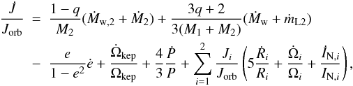 (6)or
even the simpler form proposed by Tout & Hall (1991, hereafter TH91):
(6)or
even the simpler form proposed by Tout & Hall (1991, hereafter TH91):  (7)In both Eqs. (6) and (7), M1 and M2 are the
masses of the primary and the secondary component, respectively. Concerning the
relation of TH91 (Eq. (7)),
Ṁ2 > 0 is the mass rate accreted by
the gainer through the L1 point, Ṁ < 0 is the
remaining ML rate escaped by the donor out of the system, Jorb
is the orbital angular momentum,
(7)In both Eqs. (6) and (7), M1 and M2 are the
masses of the primary and the secondary component, respectively. Concerning the
relation of TH91 (Eq. (7)),
Ṁ2 > 0 is the mass rate accreted by
the gainer through the L1 point, Ṁ < 0 is the
remaining ML rate escaped by the donor out of the system, Jorb
is the orbital angular momentum,  is the angular momentum lost by the system and P is the orbital period.
In the
relation of KRL06 (Eq. (6)), ML driven by
stellar winds is allowed by both components at a total rate of
Ṁw = Ṁw,1 + Ṁw,2 < 0.
Moreover, the
relation of Eq. (6) includes terms connected
to ML via the L2 point, eccentricity variations, and changes in parameters related to the
internal structure of the components.
In particular, Ji,
Ωi, Ri and
IN,i
(i = 1,2) are the angular momentum, the angular
velocity, the stellar radius (radius of equivalent volume) and the normalized moment of
inertia of each component, respectively, while q, Ωkep and
e are the mass ratio, the Keplerian angular velocity and the eccentricity
of the system. The term ṁL2 accounts for the ML via L2 and
Ṙi,
İN,i for the internal structure
evolutionary changes. Finally,  ,
,
 ,
ė and Ṗ accounts for the orbital changes.
,
ė and Ṗ accounts for the orbital changes.
Our present analysis will be limited to detached systems (so that mass exchange will be
excluded) consisting of late-type main-sequence stars with circular orbits and synchronized
components that will be furthermore assumed to be in tidal equilibrium. That is, we consider
Eqs. (6) and (7) under the conditions
Ṁ2 = ṁL2 = ė = e = 0
and
Ω1 = Ω2 = Ωkep = 2π/P,
which imply that  is valid. Because our calculations deal with time windows directly comparable with the span
of O–C diagrams (centuries at the most), stellar radii and moments of inertia evolutionary
changes will be ignored
(Ṙi = İN,i = 0).
is valid. Because our calculations deal with time windows directly comparable with the span
of O–C diagrams (centuries at the most), stellar radii and moments of inertia evolutionary
changes will be ignored
(Ṙi = İN,i = 0).
In those cases where the orbital radius is much greater than any component radius (which is
usually the case in detached binaries), we may disregard any spin contribution to the total
angular momentum of the system, leading Eqs. (6) and (7) to differ only in the ML
part:  for
the KRL06 and TH91 approach, respectively.
for
the KRL06 and TH91 approach, respectively.
Because
\(J_\mathrm{orb}=M_\mathrm{red}A_\mathrm{orb}^{2}\Omega_\mathrm{kep}\)
, where
Mred = M1M2/(M1 + M2)
is the reduced mass of the system and
Aorb = G1/3(M1 + M2)1/3P2/3/(2π)2/3
is the orbital radius, we also have  (10)Equation (10) reveals a close connection between the
orbital angular momentum and the period of the system. Non-conservative ML mechanisms
increase the orbital period, while angular momentum loss (AML) processes, such as MB and
gravitational radiation, lead to a period reduction.
(10)Equation (10) reveals a close connection between the
orbital angular momentum and the period of the system. Non-conservative ML mechanisms
increase the orbital period, while angular momentum loss (AML) processes, such as MB and
gravitational radiation, lead to a period reduction.
3. Mathematical procedure
To find analytically the morphology of synthetic O–C diagrams under the influence of
certain physical mechanisms, we have to solve analytically the differential Eq. (5) for ΔT(ϵ).
This will be performed when various forms of P(ϵ) function
on the l.h.s. of Eq. (5) have been specified
theoretically through the
relations. Thus, first we apply Eqs. (6)
and (7) for each individual physical
mechanism that drives the orbital evolution and solve for the orbital period
P(t). Then, by means of Eq. (4), which provides a
t = t(ϵ) transformation, the
P(t) function can be expressed in terms of the variable
ϵ in a P(ϵ) form. In consequence,
P(ϵ) can be substituted into the differential Eq. (5), whose solution, under the initial conditions
(ϵ,t,ΔT(ϵ),P(ϵ)) = (0,T0,0,Pe),
will provide the ΔT(ϵ) function in its analytical form.
The ΔT(ϵ) function indeed describes the O–C diagram in its
usual meaning.
Because the construction of O–C diagrams suffer from errors attributed either to times of
minima rough determination (e.g. based on visual and patrol plates observations) or stellar
activity that distorts even a very accurate determination (e.g. dark or bright features on
stellar photospheres and atmospheres such as spots and plages), a significant scatter
commonly appears. An O–C signal is then detectable when the
ΔT(ϵ) function, determined for a certain mechanism, is
at least comparable to the noise level of the diagram, ε. The critical
minimum number of epochs needed for this condition to be reached,
ϵmin (and so, the equivalent minimum temporal interval
t(ϵmin) − T0
directly through transformation Eq. (4)), can
be derived then by solving the equation  (11)The choice of the noise
level in O–C diagrams constitutes an interesting aspect that deserves our attention and
discussion. Noise in O–C diagrams has two main components: (a)
time-of-minimum-light misdeterminations (usually caused by asymmetric minimum profiles and
low-quality observations) and (b) heterogeneities in the radiation field of
the stellar surfaces (usually caused by solar-type magnetic activity).
(11)The choice of the noise
level in O–C diagrams constitutes an interesting aspect that deserves our attention and
discussion. Noise in O–C diagrams has two main components: (a)
time-of-minimum-light misdeterminations (usually caused by asymmetric minimum profiles and
low-quality observations) and (b) heterogeneities in the radiation field of
the stellar surfaces (usually caused by solar-type magnetic activity).
Our general experience of the determination of a minimum time through methods suitable for symmetric minima such as the Kwee & van Woerden (1956) or parabola-fitting methods (Breinhorst et al. 1973) is that a standard error of the order of 0.001 d is expected by the procedure when photoelectric observations are used. The situation becomes much worse when the determination is performed by means of photographic photometry and becomes remarkably doubtful when the whole process is based on visual or patrol plate observations. The error may be increased by a factor of ten or even thirty in the former and the latter case, respectively (e.g. Mallama 1974a, b; Duerbeck 1975; Hall & Kreiner 1980). Apart from these errors, whose nature is purely statistical, the photometric noise caused by the heterogeneous surface of the stellar components, characterizing mainly late-type stars, is able to misguide any inference from O–C diagrams analysis. It is expected that photometric noise does not exceed 0.01 d when migrating spots drift on the surface of a binary component (Ogloza 1997; Kalimeris et al. 2002).
Because none of the aforementioned noise sources directly entangles with dissipative
processes, the temporal modulation of noise amplitude is not characterized by persistency (a
property where a variation in any state parameter of a system with a certain thermal
relaxation time tends to be followed by a change of the same sign, e.g. see Allen &
Smith 1996). In this case, errors as those involved in
the O–C differences are not autocorrelated by any way but retain a random character. Hence,
the aforementioned error components are expected to be Gaussian in their nature and to
follow a normal distribution
N(μ,σε)
with mean μ = 0 and variance  . As a
consequence, the O–C differences look like – and are indeed – a signal embedded in a
white-noise background, while the noise level (or power density) ε will be
statistically determined by σε. In this
context, ε could be also determined directly from the observed O–C diagrams
of a system by applying a combination of spectral analysis methods such as the maximum
entropy (Burg 1967; Haykin & Kessler 1983), multi-taper (Thomson 1982; Mann & Lees 1996)
and Monte Carlo singular spectral analysis (Allen & Smith 1996; Broomhead & King 1986).
. As a
consequence, the O–C differences look like – and are indeed – a signal embedded in a
white-noise background, while the noise level (or power density) ε will be
statistically determined by σε. In this
context, ε could be also determined directly from the observed O–C diagrams
of a system by applying a combination of spectral analysis methods such as the maximum
entropy (Burg 1967; Haykin & Kessler 1983), multi-taper (Thomson 1982; Mann & Lees 1996)
and Monte Carlo singular spectral analysis (Allen & Smith 1996; Broomhead & King 1986).
In the context of the aforementioned discussion, the value of ε = 0.001d is considered here as a typical lowest bound, the one of ε = 0.03d as a typical upper bound and ε = 0.01d as our pilot statistical noise level (e.g. for cases where it might not be clear whether the photometric noise is exclusively affecting our observations).
4. Examination of physical mechanisms
The above mathematical methodology is implemented for stellar-wind-driven ML and MB in the first and second subsection respectively. Finally, in another (third) subsection, we regard the combined action of both mechanisms to derive simple analytical conditions, suitably applied to any late-type detached binary system, that determine which mechanism dominates.
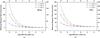 |
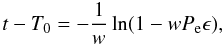
Fig. 1 Minimum time spans for several mass loss rates based on the KRL06 a) and TH91 b) approach. Computations were performed for noise level equal to 0.001 d (squares), 0.01 d (crosses) and 0.03 d (up triangles). (This figure is available in color in the electronic form.) |
4.1. Case I: Mass loss through stellar wind
In late-type stars, stellar luminosity is the most important factor that dictates the development of thermally driven winds. In the literature many semi-empirical relations have been evoked which allow the estimation of their ML rate, Ṁw, through their absolute parameters and evolutionary state that (either directly or indirectly) determine the luminosity contribution (e.g. Lednicka & Stȩpień 2008; Reimers 1975; Reimers 1977; de Jager et al. 1988; Schröder & Cuntz 2005). In close binary systems, the wind-driven ML rate appears to be much more enhanced than the single-star counterpart once (a) tidal interaction is strong enough to keep the spin locked at (high) orbital angular velocities and (b) the components approach their Roche lobe radii, RL, i (e.g. Eggleton 1983; Tout & Eggleton 1988; Eggleton 1992; Hilditch 2001).
However, because even dynamical or thermal timescale ML rates do not exceed
−10-4 M⊙ yr-1 and
−10-6 M⊙ yr-1 respectively (see for
instance Hilditch 2001), we may safely assume that
Ṁw,i is constant and small enough to affect
the absolute parameters of any of the components as long as binaries are monitored by
means of O–C diagrams. Hence, the
relation, given by Eq. (8) or (9), is reduced to an ordinary first-order
differential equation of the form  (12)where
 (13)for the KRL06 approach.
Note that w is estimated through Eq. (13) by tacitly assuming that no AML occurs through the gas lost caused
by the ML itself (i.e.  )
because magnetic braking is the mechanism that dominates this process. Under this regime,
the quantity K which appears in TH91, is set as
)
because magnetic braking is the mechanism that dominates this process. Under this regime,
the quantity K which appears in TH91, is set as
 (see Eq. (20) of their paper) and, as a consequence, w takes the
simplified form
(see Eq. (20) of their paper) and, as a consequence, w takes the
simplified form  (14)for the TH91 approach.
The solution of Eq. (12) under the
initial condition
(t,P(t)) = (T0,Pe)
is  (15)Then, integration
of Eq. (4) under the initial condition
(ϵ,t) = (0,T0) yields
(15)Then, integration
of Eq. (4) under the initial condition
(ϵ,t) = (0,T0) yields
 (16)and so,
 (17)Integration of Eq. (5) under the initial condition
(ϵ,ΔT(ϵ)) = (0,0)
eventually gives the ΔT(ϵ) function
(17)Integration of Eq. (5) under the initial condition
(ϵ,ΔT(ϵ)) = (0,0)
eventually gives the ΔT(ϵ) function  (18)which is
convex for any ϵ referring to the increasing
orbital period function P(ϵ), expressed by
relation Eq. (17).
(18)which is
convex for any ϵ referring to the increasing
orbital period function P(ϵ), expressed by
relation Eq. (17).
Given the ΔT(ϵ) function, Eq. (11) can be solved numerically by a Newton-Raphson procedure (e.g. Press et al. 1992) to determine the minimum time intervals required for the detection of an O–C signal driven by the ML mechanism in any detached system. Our test case, for example, concerns a typical short-period RS CVn-type binary, i.e. M1 = M2 = M⊙, R1 = R2 = R⊙ and Pe = 1d. We have performed calculations for several ML rates adopting our pilot noise level of 0.01 d (Table 1). Similar computations were also made for ε equal to 0.001 d and 0.03 d according to the KRL06 (Fig. 1a) and TH91 approach (Fig. 1b), respectively. It is important to note that the inferred intervals do not depend on the reference period because the latter contributes to Eq. (18) only by the term Peϵ, which is a pure function of t − T0 according to the relation in Eq. (16).
Minimum time spans for several mass loss rates based on the KRL06 and TH91 approach at ε = 0.01d (see text for details).
The first approach concerns ML by both components without any additional restriction and hence, systems consisted of members with competitive ML rates may constitute the appropriate candidates for its proper applications (e.g. a pair of stars with similar evolutionary state). In contrast, the second approach focuses on wind-driven ML by only one of the components, a property that restricts its applications to cases of components with great difference on ML rates (e.g. a pair of stars with different evolutionary state). For instance, binaries belonging to the short-period RS CVn group, consisting of main-sequence stars only (Budding & Zeilik 1987), could be suitable for the KRL06 approach, while typical RS CVn-type systems, consisting of a primary dwarf and a secondary subgiant (Popper & Ulrich 1977), might be recommended for the TH91 approach.
Given that O–C diagrams contain data that marginally exceed observations of a century, the aforementioned results render clear that a convex O–C signal can be easily ascribed to ML effects with rates greater than −10-10 M⊙ yr-1, assuming the lowest noise level of ε = 0.001d. Supposing that the respective level increases to ε = 0.01 or 0.03 d, ML is rendered measurable only when its rate is greater than −10-9 M⊙ yr-1. This finding agrees with traditional approaches followed so far where a typical ML rate ranges within −10-9 and −10-6 M⊙ yr-1 (e.g. Hall & Kreiner 1980).
4.2. Case II: Angular momentum loss through magnetic braking
Magnetic stellar winds cause both mass and angular momentum loss in low-mass stars via MB mechanism. Stellar material, kept by strong magnetic fields, corotates with the star up to a distance determined by the Alfvén radius (dead zone). The material escapes out of this region in a steep way producing the well-known stellar wind (wind zone). As far as main-sequence stars are concerned, the magnetic nature of a wind holds when a deep convective envelope exists, a property that characterizes late-type spectral types (F0 or later) or, equivalently, dwarf stars with mass less than approximately 1.5M⊙.
From a theoretical point of view, the braking mechanism is expected to depend on the
strength of the magnetic field, the Alfvén radius, the extent of stellar wind (Schatzman
1962; Mestel 1968), and also on the geometry of the stellar magnetic field with the degree of
its stiffness at long distances from the star to play a principal role (Mestel 1984). By following different approaches, we may
establish generalized and flexible power laws of the form
 ,
with a being positive constant (e.g. Weber & Davis 1967; Okamoto 1974; Mestel 1984; Mestel &
Spruit 1987; Kawaler 1988). A problem that arises with all these theoretical approaches is
the involvement of too many physical quantities for which our knowledge is limited, which
renders them unsuitable for a wide spectrum of applications. Instead, we may reproduce the
aforementioned power laws of AML as a function of angular velocity and ML rate by
calibrating some constants according to observational constraints and leaving just a few
parameters free (e.g. Verbunt & Zwaan 1981;
Vilhu 1982; Rappaport et al. 1983; Mestel 1984; Kawaler 1988; van’t Veer & Maceroni 1989; Vilhu 1992; Stȩpień 1995). An alternative way of
estimating the AML rate is also the use of empirical relations that would connect the
magnetic torque with the level of X-ray activity (e.g. Vilhu 1994; Ivanova & Taam 2003) considering that a correlation between AML and X-ray luminosity is
expected to exist (e.g. Moss 1986; Vilhu &
Moss 1986; Mestel & Spruit 1987).
,
with a being positive constant (e.g. Weber & Davis 1967; Okamoto 1974; Mestel 1984; Mestel &
Spruit 1987; Kawaler 1988). A problem that arises with all these theoretical approaches is
the involvement of too many physical quantities for which our knowledge is limited, which
renders them unsuitable for a wide spectrum of applications. Instead, we may reproduce the
aforementioned power laws of AML as a function of angular velocity and ML rate by
calibrating some constants according to observational constraints and leaving just a few
parameters free (e.g. Verbunt & Zwaan 1981;
Vilhu 1982; Rappaport et al. 1983; Mestel 1984; Kawaler 1988; van’t Veer & Maceroni 1989; Vilhu 1992; Stȩpień 1995). An alternative way of
estimating the AML rate is also the use of empirical relations that would connect the
magnetic torque with the level of X-ray activity (e.g. Vilhu 1994; Ivanova & Taam 2003) considering that a correlation between AML and X-ray luminosity is
expected to exist (e.g. Moss 1986; Vilhu &
Moss 1986; Mestel & Spruit 1987).
The determination of the exponent a constitutes a subject of crucial
importance owing to its connection with rotation itself. Slow rotators seem to be
consistent with a value of a equal to 3, as was theoretically predicted
by Weber & Davis (1967) and observationally
supported by Skumanich (1972) and many other
similar studies (e.g. Smith 1979; Soderblom 1982; Soderblom 1983; Stauffer 1987; Stauffer &
Hartmann 1987), while the value
a = 2 cannot be excluded for moderate rotators (Mayor &
Mermilliod 1991; Charbonneau 1992; Keppens et al. 1995).
However, for rapidly rotating stars AML, induced by MB, is believed to be reduced (e.g.
Rucinski 1983; Vilhu & Moss 1986; Mestel & Spruit 1987; Taam & Spruit 1989) because of a possible saturation of the magnetic field, i.e. independence of
its strength by the angular velocity (e.g. Vilhu & Walter 1987; Stȩpień 1991; Pizzolato
et al. 2003), resulting in AML laws with the
exponent a close to unity, i.e.  .
Recently, there have been remarkable advanced theoretical studies supporting a rotation in
solar-type stars that is far from homogeneous (see Krishnamurthi et al. 1997; Allain 1998; Irwin & Bouvier 2009, for
excellent reviews on this topic), a key factor whose contribution is substantial for the
calibration of the final AML parametrization. In this case, a combination of all three
aforementioned exponents turns out to be the most efficient choice (e.g. Barnes &
Sofia 1996; Allain 1998). It is also worthwhile to point out that the critical value of angular
velocity over which the saturated law is implemented appears to be strongly mass-dependent
(Pinsonneault et al. 1989; Barnes & Sofia
1996; Krishnamurthi et al. 1997; Allain 1998).
.
Recently, there have been remarkable advanced theoretical studies supporting a rotation in
solar-type stars that is far from homogeneous (see Krishnamurthi et al. 1997; Allain 1998; Irwin & Bouvier 2009, for
excellent reviews on this topic), a key factor whose contribution is substantial for the
calibration of the final AML parametrization. In this case, a combination of all three
aforementioned exponents turns out to be the most efficient choice (e.g. Barnes &
Sofia 1996; Allain 1998). It is also worthwhile to point out that the critical value of angular
velocity over which the saturated law is implemented appears to be strongly mass-dependent
(Pinsonneault et al. 1989; Barnes & Sofia
1996; Krishnamurthi et al. 1997; Allain 1998).
All the aforementioned models adapt single cool stars containing thick convective zones so that the stellar dynamo is able to offer the necessary requirements for the braking mechanism. The star loses angular momentum in a way dictated by its spectral type, leading to a decreasing spin as a direct result. The situation is completely reversed if a late-type star belongs to a close pair. Assuming a tidally locked binary system, presumable AML of any member should occur at the expense of the orbital angular momentum because of the spin-orbit coupling, leading to period decrease and, hence, to spinning up both of the two companions. Typical values for the exponent a, derived by studies in close binary systems, show that the AML regime of the stars belonging to a close pair is close to the saturated one, e.g. a = 1.6 (Vilhu 1992), a = 1.3 (Ivanova & Taam 2003), a = 1.2 (Rucinski 1983) and a = 0.5 (van’t Veer & Maceroni 1988).
4.2.1. Adopted formalism
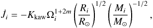
Here, we essentially adopt the parametrization of Kawaler (1988) because of its simple, flexible and condensed form. Based on
the Mestel (1984) and Mestel & Spruit
(1987) findings, Kawaler (1988) employs a power law
B ∝ Ωm holding for the magnetic field
strength B that finally leads to the following AML law:  (19)where
Kkaw is a positive constant, highly dependent on
a, containing all of our ignorance about winds and magnetic field
generation in stars (it is estimated after appropriate calibration as usual),
M, R and Ṁ are the stellar mass,
radius and ML rate, respectively, m expresses the degree of field
strength depending on the angular velocity (for instance, m = 1
accounts for the Skumanich law and m = 0 for the saturation law) and
n assimilates to the field geometry (for instance,
n = 3/7 accounts for a dipole field and
n = 2 for a radial field). The value
n = 3/2 is compatible with the Skumanich law and
close to radial field topology.
(19)where
Kkaw is a positive constant, highly dependent on
a, containing all of our ignorance about winds and magnetic field
generation in stars (it is estimated after appropriate calibration as usual),
M, R and Ṁ are the stellar mass,
radius and ML rate, respectively, m expresses the degree of field
strength depending on the angular velocity (for instance, m = 1
accounts for the Skumanich law and m = 0 for the saturation law) and
n assimilates to the field geometry (for instance,
n = 3/7 accounts for a dipole field and
n = 2 for a radial field). The value
n = 3/2 is compatible with the Skumanich law and
close to radial field topology.
Because we cannot yet be sure which value we should choose as the most appropriate in
our computations, here we followed the suggestion of Kawaler (1988) that the value n = 3/2
corresponds to an intermediate field geometry, which was also mentioned by Allain (1998). In this case, the braking law does not depend
anymore on the pace at which the star loses mass and eventually obtains the reduced form
 (20)which is tantamount to
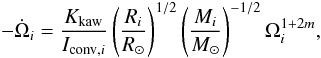
 (21)or equivalently,
 (22)where
 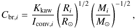 (23)a = 1 + 2m
and
(23)a = 1 + 2m
and  is the
moment of the convective envelope inertia for each
i = 1,2 member of a binary system when
ki is their respective dimensional
gyration radius. We decided to use this formalism owing to its compatibility with
various braking laws found in literature, as is shown in the following paragraphs.
is the
moment of the convective envelope inertia for each
i = 1,2 member of a binary system when
ki is their respective dimensional
gyration radius. We decided to use this formalism owing to its compatibility with
various braking laws found in literature, as is shown in the following paragraphs.
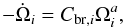
By ignoring the ML terms in either Eq. (8) or (9), considering the
assumptions reported in the first section and substituting each magnetic torque
 by
by  ,
the differential equation we have to solve is
,
the differential equation we have to solve is 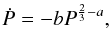 (24)after introducing
the constant quantity b as
(24)after introducing
the constant quantity b as ![\begin{equation} \label{equation:25} b=\frac{3(2\pi)^{a+\frac{1}{3}}(M_\mathrm{1}+M_\mathrm{2})^{1/3} \sum_{i=1}^{2}\left[C_{\mathrm{br},i}(k_{i}R_{i})^{2}M_{i}\right]} {M_\mathrm{1}M_\mathrm{2}G^{2/3}}>0. \end{equation}](/articles/aa/full_html/2011/11/aa16707-11/aa16707-11-eq166.png) (25)The solution of
Eq. (24) under the initial condition
(t,P(t)) = (T0,Pe)
is
(25)The solution of
Eq. (24) under the initial condition
(t,P(t)) = (T0,Pe)
is ![\begin{equation} \label{equation:26} P(t)=\left[P_\mathrm{e}^{a+\frac{1}{3}}-b\left(a+\frac{1}{3}\right) (t-T_\mathrm{0})\right]^{\frac{1}{a+\frac{1}{3}}}. \end{equation}](/articles/aa/full_html/2011/11/aa16707-11/aa16707-11-eq167.png) (26)Then, integration of
Eq. (4) under the initial condition
(ϵ,t) = (0,T0) yields
(26)Then, integration of
Eq. (4) under the initial condition
(ϵ,t) = (0,T0) yields
![\begin{equation} \label{equation:27} t-T_\mathrm{0}=\frac{1}{b\left(a+\frac{1}{3}\right)} \left\{P_\mathrm{e}^{a+\frac{1}{3}}-\left[P_\mathrm{e}^{a-\frac{2}{3}} -b\left(a-\frac{2}{3}\right)\epsilon\right]^{\frac{a+\frac{1}{3}} {a-\frac{2}{3}}}\right\}, \end{equation}](/articles/aa/full_html/2011/11/aa16707-11/aa16707-11-eq168.png) (27)and so,
(27)and so, ![\begin{equation} \label{equation:28} P(\epsilon)=\left[P_\mathrm{e}^{a-\frac{2}{3}}-b\left(a-\frac{2}{3}\right) \epsilon\right]^{\frac{1}{a-\frac{2}{3}}}. \end{equation}](/articles/aa/full_html/2011/11/aa16707-11/aa16707-11-eq169.png) (28)Integration of
Eq. (5) under the initial condition
(ϵ,ΔT(ϵ)) = (0,0)
finally gives the ΔT(ϵ) function
(28)Integration of
Eq. (5) under the initial condition
(ϵ,ΔT(ϵ)) = (0,0)
finally gives the ΔT(ϵ) function ![\begin{eqnarray} \label{equation:29} \Delta T(\epsilon)=\frac{1}{b\left(a\!+\!\frac{1}{3}\right)} \left\{P_\mathrm{e}^{a\!+\!\frac{1}{3}}\!-\!\left[P_\mathrm{e}^{a\!-\!\frac{2}{3}} \!-\!b\left(a\!-\!\frac{2}{3}\right)\epsilon\right]^{\frac{a+\frac{1}{3}} {a-\frac{2}{3}}}\right\} -P_\mathrm{e}\epsilon, \end{eqnarray}](/articles/aa/full_html/2011/11/aa16707-11/aa16707-11-eq172.png) (29)which
is concave for any cycle ϵ referring to the
decreasing orbital period function
P(ϵ), expressed by relation Eq. (28).
(29)which
is concave for any cycle ϵ referring to the
decreasing orbital period function
P(ϵ), expressed by relation Eq. (28).
4.2.2. Choice of the braking law
At this point, we concentrate our work on the estimation of the coefficients Cbr following three different procedures found in literature. Precise determination of these coefficients is a subject of crucial importance when we have to deal with narrow time-windows of the order of a century, such as those we handle in the present study.
At first, we aim to compute the parameter Kkaw as a
function of the exponent a, i.e.
Kkaw = Kkaw(a).
Because Kkaw is essentially adjusted according to the field
geometry, a seems to be the most representative variable to modulate
Kkaw. Hence, adopting the formalism used by Allain (1998), Kkaw is converted
into the Skumanich constant, Ksk, and the one of
Mayor-Mermillod, Kmm, at a = 3 and
a = 2, respectively. The next two methodologies out of the three in
total deal with solar-like stars and, as a result, Kkaw may
be readily estimated by the formula  (30)provided that
Cbr(a) is somehow already known.
(30)provided that
Cbr(a) is somehow already known.
The first approach concerns the one adopted by Vilhu (1982, hereafter V82). In that paper, V82 calibrates the well-known Skumanich
formula at the age of the Pleiades, considering that the mean observed rotational
velocity for solar-type stars is about
vPl = 20kms-1. The author proposes a
semi-empirical relation that estimates the AML rate for a single star with reference to
the respective rate observed in the Pleiades at present,
 ,
directly connected with its rotational period and the exponent a.
Indeed, the period, given as a fraction of 3 d, is raised to a. This
term is introduced by hand to be valid with rotators whose period is shorter than 3 d by
picking values among 1, 2 or 3 for a:
,
directly connected with its rotational period and the exponent a.
Indeed, the period, given as a fraction of 3 d, is raised to a. This
term is introduced by hand to be valid with rotators whose period is shorter than 3 d by
picking values among 1, 2 or 3 for a: 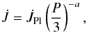 (31)where
P is the period in d.
(31)where
P is the period in d.
Conducting some simple mathematical operations based on the Skumanich law,
v = cskt−1/2
leads to  and thus
is determined by adopting solar parameters for the mean rotational behaviour of the
Pleiades cluster:
and thus
is determined by adopting solar parameters for the mean rotational behaviour of the
Pleiades cluster: 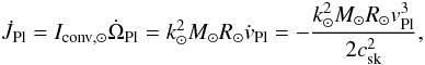 (32)where
 is
the Skumanich constant.
is
the Skumanich constant.
Setting the age of tPl = 50 Myr for the Pleiades cluster,
V82 estimated
equal to 2 × 1041 g cm2 s-1 yr-1. However, the
age of this cluster has been the subject of discussion since Basri et al. (1996) have investigated the lithium abundance of some
faint stars, members of the cluster, resulting a much older age of about 115 Myr. After
it is harmonised with the present perception of 100 Myr as an average age, which is
widely accepted by many studies (e.g. Soderblom et al. 1993; Queloz et al. 1998),
is halved to the value 1041 g cm2 s-1 yr-1.
Relation Eq. (31) is consistent with
the spin-down law of Eq. (22) with
coefficients Cbr to be given by the formula  (33)in
sa−2 and thus,
(33)in
sa−2 and thus,  (34)in
g cm2 sa−2.
(34)in
g cm2 sa−2.
The second approach we are employing concerns the one presented in van’t Veer &
Maceroni (1989, hereafter VVM89). In that work,
VVM89 suggest an estimation of Cbr coefficients directly
through the braking law Eq. (22) itself.
This can be done by considering two clusters of similar ages and supposing that the mean
rotational regime of the older cluster is another evolutionary stage of the younger one,
driven by AML. After a simple integration of Eq. (22), VVM89 proposed the estimation of coefficients
Cbr via the formula  (35)and
thus,
(35)and
thus,  (36)where Ω1,
Ω2 account for the mean angular velocity of solar-type stars in the younger
and the older cluster respectively; v1,
v2 account for their respective mean rotational velocity
and t1, t2 correspond to their
ages.
(36)where Ω1,
Ω2 account for the mean angular velocity of solar-type stars in the younger
and the older cluster respectively; v1,
v2 account for their respective mean rotational velocity
and t1, t2 correspond to their
ages.
In VVM89, application of relation Eq. (36) takes place for the clusters a Per (~50 Myr) and Pleiades (~70 Myr), adopting mean rotational velocities by Stauffer (1987) according to whom the velocity drops from 200 to 10 km s-1 in a short temporal interval of about 20 Myr (set approximately as 10 Myr in their original paper). Here, we recalibrate equation Eq. (36), assuming that the average age of the Pleiades is close to 100 Myr and so the time within which the stars attain the velocity of 10 km s-1 increases to 50 Myr. Especially at a = 1, Kkaw cannot be determined by Eq. (36) because of its irregular properties. To overcome this difficulty, we used de l’Hospital rule, which led to [(k⊙R⊙)2 M⊙/(t2 − t1)] ln(v1/v2), which we adopted in our calculations.
The third approach concerns a much more complicated procedure with respect to the two previous ones. We will not consider this because the procedure aims to calibrate braking laws using codes of AML evolution. Computations take into account the effect of envelope-core decoupling and propose the best Kkaw and Cbr values to achieve the optimal fit with observations, usually spanning the whole Hayashi contraction track. Here we fully adopt the values of Kkaw inferred by Allain (1998, hereafter A98). This author has used AML evolutionary codes (Forestini 1994; Bouvier et al. 1997) to include internal angular momentum transfer (e.g. Endal & Sofia 1981; MacGregor & Brenner 1991; Keppens et al. 1995). Computations have been made for 1.0, 0.8, 0.6 and 0.5M⊙ with initial period 8 d because this value corresponds to the mean observed peak of classical T Tauri stars. She has assumed that the period remains constant as long as the protostar experiences the disk-locking phase and, eventually, she has adopted Kawaler (1988) parametrization to describe the AML evolution up to the main sequence. The author has then taken into consideration recent observational constraints that emerged from the study of many young clusters to date (IC2602, IC2391, a Per, Pleiades, M7, M34 and Hyades) to provide useful information about the disk-locking phase duration, over whose critical velocities the braking law saturates as well as the envelope-core coupling timescales.
Kkaw coefficients predicted according to the braking law of V82, VVM89, and A98 for the entire range in which exponent a lies.
Towards the main sequence, A98 has used three laws to describe the braking mechanism.
Specifically, she has adopted the parametrization of Kawaler (1988) setting only three available exponents a
(Skumanich law for a = 3, Mayor-Mermilliod law for
a = 2 and saturation law for a = 1) and allowing a
transition among the laws provided that some criteria regarding the angular velocity are
fulfilled:  (37)when
a = 3 and
Ω < Ωcrit = Kmm/Ksk,
(37)when
a = 3 and
Ω < Ωcrit = Kmm/Ksk,
 (38)when
a = 2 and
Ωcrit ≤ Ω < Ωsat and
(38)when
a = 2 and
Ωcrit ≤ Ω < Ωsat and  (39)when
a = 1, Ω ≥ Ωsat and
Ksat = Kmm Ωsat.
(39)when
a = 1, Ω ≥ Ωsat and
Ksat = Kmm Ωsat.
Short coupling timescales (SCT) have led to Ksk = 2.25 × 1047 g cm2 s, Kmm = 4.2 × 1042 g cm2 and Ωsat = 35 Ω⊙ for the 1 M⊙ calibration with Ωsat = 15 Ω⊙, 10 Ω⊙ and 2.6 Ω⊙ for the 0.8 M⊙, 0.6 M⊙ and 0.5 M⊙ calibration, respectively. Intermediate coupling timescales (ICT) have led to Ksk = 2.7 × 1047 g cm2 s, Kmm = 4.2 × 1042 g cm2 and Ωsat = 30 Ω⊙ for the 1 M⊙ calibration with Ωsat = 15 Ω⊙, 10 Ω⊙ and 2.7 Ω⊙ for the 0.8 M⊙, 0.6 M⊙ and 0.5 M⊙ calibration, respectively, revealing negligible changes in the values. Finally, long coupling timescales (LCT) have determined the incorporated parameters as Ksk = 1.5 × 1048 g cm2 s, Kmm = 6.3 × 1042 g cm2 and Ωsat = 6 Ω⊙ for the 1 M⊙ calibration with Ωsat = 5 Ω⊙, 4 Ω⊙ and 1.2 Ω⊙ for the 0.8 M⊙, 0.6 M⊙ and 0.5 M⊙ calibration, respectively (A98).
In Table 2 we tabulated the estimates of the Kkaw coefficients according to the three approaches presented above. Among them, the A98 computations are considered to be the most valid because they have taken into account recent theoretical developments and the latest observational constraints and, as a consequence, our reference values are those predicted by A98. In that sense, VVM89 appears to overestimate Kkaw coefficients almost along the whole range of a considered. However, none of the deduced declinations exceeds one order of magnitude (apart from the saturation regime where it is slightly exceeded). On the other hand, the V82 approach seems to follow that of A98 in a very satisfactory agreement and, hence, it seems to be the most efficient choice when intermediary exponents are needed.
We now proceed to the estimation of the minimum time needed to measure an O–C signal
induced by the MB mechanism. To do this, we solved Eq. (11) by means of a Newton-Raphson procedure, similarly to the
wind-driven ML case. Solar parameters for a typical short-period RS CVn-type binary,
i.e.
M1 = M2 = M⊙,
R1 = R2 = R⊙,
 and
Pe = 1d, were adopted and a typical noise level equal to
ε = 0.01d was assumed to contaminate our observations. Our results
are tabulated in Table 3 for a variety of
exponents a when the V82, VV89 and A98 approach is employed.
and
Pe = 1d, were adopted and a typical noise level equal to
ε = 0.01d was assumed to contaminate our observations. Our results
are tabulated in Table 3 for a variety of
exponents a when the V82, VV89 and A98 approach is employed.
Minimum time spans for several values of exponent a based on the V82, VVM89, and A98 approach at ε = 0.01d (see text for details).
In contrast to the minimum required time intervals in the ML case, the time needed for disentangling the MB imprint from noise in O–C diagrams strongly depends on the period, as is easily seen in Eq. (29). Therefore, we conducted an additional investigation to find out whether MB-driven modulations can be measured in decades and, if so, to determine upper period barriers treating exponent a as a free parameter.
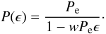
We explore all three braking laws presented above with the orbital period to vary between 0.1 d and 1.0 d by making the assumption that braking laws hold for the whole rotational range with a unique value of exponent a. Our reference noise level of ε = 0.01d was set in Eq. (11) and the ΔT(ϵ) function was adjusted by using Kkaw values from Table 2. Our results are depicted in Figs. 2a–c when the V82, VVM89 and A98 approach is selected for a = 3, 2 and 1, respectively.
 |
Fig. 2 Minimum time spans for several orbital periods and braking laws with a = 3 a), a = 2 b) and a = 1 c). The noise level is fixed at the value of 0.01 d. Squares and circles account for the V82 and VVM89 approach, respectively. Crosses, downwards pointing and right triangles account for the A98 approach when short, intermediate and long coupling timescales are considered, respectively. d) The same as c) when the noise level is reduced at the value of 0.001 d. (This figure is available in color in the electronic form.) |
A close inspection of these figures reveals that the smaller the orbital period, the shorter is the time required. Observed period changes might be ascribed to MB in very short-period binaries such as contact systems and cataclysmic variables with periods less than about 0.5 d. In this group of binaries, we ought to expect orbital variations according to the A98 approach, regardless of the way the stellar interior rotates (Figs. 2a and b). In practice, however, any braking-induced period variation does not seem feasible because the saturation regime is expected to be achieved at periods lower than about 0.8 d (i.e. Ωsat ~ 30 Ω⊙) according to A98 (Fig. 2c). Inversely, VVM89 seem to be too optimistic in their prediction of period variations expected at the most in 150yr even for periods over than 1 d. By reducing the noise level to ε = 0.001d, most of the adopted approaches turn out to need observations spanning at the most 200yr (Fig. 2d), which gives strong reasons to believe that MB may be a candidate mechanism to drive concave variations in high-quality O–C diagrams of short and intermediate-period binaries.
4.3. Case III: Wind-driven mass loss and magnetic braking
Because the magnetic nature of stellar winds causes both ML and AML via the MB process,
their simultaneous involvement in the angular momentum evolution of a system is then
needed. Still ignoring spin angular momentum terms, either Eq. (6) or (7) leads to the differential equation  (40)with the constant
w given by Eq. (13)
or (14) for the KRL06 and TH91 approach,
respectively, and b provided by Eq. (25).
(40)with the constant
w given by Eq. (13)
or (14) for the KRL06 and TH91 approach,
respectively, and b provided by Eq. (25).
The solution of Eq. (40) under the
initial condition
(t,P(t)) = (T0,Pe)
relies on integrals that are difficult to treat but can still analytically determined:
![\begin{equation} \label{equation:41} P(t)=\left[\frac{b}{w}- \left(\frac{b}{w}-P_\mathrm{e}^{a+\frac{1}{3}}\right) \mathrm{e}^{w\left(a+\frac{1}{3}\right)(t-T_\mathrm{0})}\right] ^{\frac{1}{a+\frac{1}{3}}}. \end{equation}](/articles/aa/full_html/2011/11/aa16707-11/aa16707-11-eq318.png) (41)The
P(t) function, expressed by Eq. (41), describes the orbital evolution of a
binary consisting of cool components with wind-driven ML rates determined by the quantity
w and AML, whose rate can be estimated by adopting one of the V82,
VVM89 and A98 braking laws. The monotony of this function is defined according to whether
the ML component or that from MB dominates. More precisely, we may distinguish three
separate cases:
(41)The
P(t) function, expressed by Eq. (41), describes the orbital evolution of a
binary consisting of cool components with wind-driven ML rates determined by the quantity
w and AML, whose rate can be estimated by adopting one of the V82,
VVM89 and A98 braking laws. The monotony of this function is defined according to whether
the ML component or that from MB dominates. More precisely, we may distinguish three
separate cases: 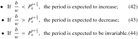 Equation (44) provides the condition under which
MB counterbalances ML in a perfect way. There are many combinations of
values accounting for w and b such that the period does
not change. In Fig. 3a we have shown some simple
examples in which synthetic O–C diagrams for a 1 d binary pair of
1 + 1 M⊙ total mass are constructed. In these diagrams we
used Eqs. (18) and (29) when ML and MB are the mechanisms driving
the orbital evolution over a range of 400yr. An ML rate of
−5 × 10⁻¹⁰ M⊙ yr-1, by adopting the
KRL06 approach for instance, seems comparable in strength to an AML mechanism with
a = 1 when the VVM89 model is implemented. In this specific case, ML
compensates the braking process, with the result that both period and O–C diagrams show no
variation (Fig. 3b). We stress that this is a
crucial finding because there are several short-period detached RS CVn-type
binaries that exhibit this peculiar attitude (e.g. YY Gem, BH Vir, UV Psc and CM Dra). It
seems likely that a joint presence of two or even more physical processes with opposite
direction holds rather than anyone at all.
Equation (44) provides the condition under which
MB counterbalances ML in a perfect way. There are many combinations of
values accounting for w and b such that the period does
not change. In Fig. 3a we have shown some simple
examples in which synthetic O–C diagrams for a 1 d binary pair of
1 + 1 M⊙ total mass are constructed. In these diagrams we
used Eqs. (18) and (29) when ML and MB are the mechanisms driving
the orbital evolution over a range of 400yr. An ML rate of
−5 × 10⁻¹⁰ M⊙ yr-1, by adopting the
KRL06 approach for instance, seems comparable in strength to an AML mechanism with
a = 1 when the VVM89 model is implemented. In this specific case, ML
compensates the braking process, with the result that both period and O–C diagrams show no
variation (Fig. 3b). We stress that this is a
crucial finding because there are several short-period detached RS CVn-type
binaries that exhibit this peculiar attitude (e.g. YY Gem, BH Vir, UV Psc and CM Dra). It
seems likely that a joint presence of two or even more physical processes with opposite
direction holds rather than anyone at all.
This does not apply detached binary systems only. Depending on the Roche configuration, on the physical features of the two members, and on possible external effects (mainly produced by unseen components), similar consequences might be achieved through a proper combination of physical processes. The AML mechanisms (e.g. magnetic braking, gravitational radiation, mass loss escape through the L2 point) can be opposed, for instance, either by an increasing fraction of a long period light-time orbit or by a mass transfer process through the L1 point when the more massive star is also the accretor.
It is worthwhile to note that integration of Eq. (41) is not feasible in analytical way and, as a result, neither the P(ϵ) nor ΔT(ϵ) function can be determined in closed form. Instead, we may insert the discrete temporal transformation that naturally results from combining Eqs. (4) and (5), i.e. t − T0 = PeE + ΔT(E), and then express the period with its discrete form, as provided by Eq. (1). As a result, cycle to cycle computations can be carried out when a numerical treatment is needed.
 |
Fig. 3 a) Synthetic O–C diagrams expected for mass loss and magnetic braking processes when the KRL06 and VVM89 approach is employed. Squares and upwards pointing triangles account for rates of −5 × 10⁻⁹ and −10-9 M⊙ yr-1, while downwards pointing triangles, diamonds, and circles account for a = 3, 2 and 1, respectively (step ≡ 4000 cycles). b) The same as a) for the combined action (crosses) of mass loss at a rate of −5 × 10⁻¹⁰ M⊙ yr-1 (circles) and magnetic braking process with a = 1 (diamonds). The respective period diagram is also displayed for both mechanisms (straight line) or each mechanism individually (dashed and dotted line, respectively). (This figure is available in color in the electronic form.) |
5. Discussion
We have presented a new methodology that allows the assessment of the detectability limits
that an O–C diagram analysis offers when long-term physical processes are examined. More
particularly, synthetic O–C diagrams may be developed by appropriate parameterized
analytical expressions, derived according to the
relation that governs a system, and evaluated under specific conditions that concern the
uncertainty and the temporal range of available observations.
A Taylorian representation of the analytical function form that describes a synthetic O–C
diagram for each particular case deserves a more detailed investigation. For instance,
considering in detail the results presented in Table 1, one can easily verify that every value regarding temporal intervals is reduced
by a factor close to  for every order of magnitude that the ML rate grows. This is so, because the quadratic term
of the Taylorian polynomial seems satisfactory to represent the function Eq. (18) with sufficient accuracy. The limits within
which a parabolic curve adequately represents the observed long-term modulations in O–C
diagrams will be provided in a forthcoming paper.
for every order of magnitude that the ML rate grows. This is so, because the quadratic term
of the Taylorian polynomial seems satisfactory to represent the function Eq. (18) with sufficient accuracy. The limits within
which a parabolic curve adequately represents the observed long-term modulations in O–C
diagrams will be provided in a forthcoming paper.
Apart from the well-examined wind-driven ML process, we have thoroughly investigated the feasibility of the current O–C diagrams to detect the presence of MB mechanism. When strong AML dependence on rotation exists, i.e. a ~ 3, almost any examined approach leads to time spans short enough to be covered by the current O–C diagrams. When this dependence drops to a ~ 2, the situation changes in a significant level and only systems with periods of less than 0.5 d seem to safely be in the temporal range of O–C diagrams. However, any period variation is hidden in noise when the saturation regime is reached, i.e. a ~ 1. A remarkable exception in the two previous cases is the VVM89 approach, which is not affected by the most pessimistic predictions of V82 and A98. Surprisingly, it estimates that no matter which a value is adopted, the corresponding short-period binary systems exhibit a clear signal in O–C diagrams up to a maximum of 150yr. An analogous situation exists when the noise level is supposed to reflect observational only uncertainties of photoelectrically determined times of minimum, regardless of the employed braking law.
Attempting to give a reasonable explanation to this considerable deviation, we recall that VVM89 restrict their calculations to a very limited time interval of about 50 Myr, which is the age difference between the Pleiades and the a Per cluster. Obviously, any decrease in rotational velocities, assumed by the available statistical studies, modulates in a very sensitive way the minimum required time intervals within which MB traces can be seen. The general framework, which the most recent investigations follow, copes with the bimodal character of rotational velocities observed in young open clusters. In the a Per cluster for instance, velocities of solar-type stars extend from a few km s-1 up to 200 km s-1, which was indeed taken into account by VVM89. However, in the Pleiades cluster, the upper limit of the group of rapid rotators has decreased to 50 km s-1, while that of slow rotators presents velocities close to 10 km s-1 (e.g. Queloz et al. 1998). van’t Veer & Maceroni (1989) have adopted that the mean velocity of 200 km s-1 in the a Per drops to 10 km s-1 in the Pleiades without making any distinction as to which group they refer. As a consequence, solar-type stars appear to decelerate at an extremely rapid pace and in a very short time, leading to a spuriously sturdy AML-rotation connection.
Nevertheless, we cannot diminish the credibility of the VVM89 results because a specific braking law seems more likely to be valid when used for time spans of a few tens of Myr rather than for temporal intervals comparable to clusters ages (i.e. for several tens or even hundreds of Myr). This approach appears to be the most convenient, whereas the one of V82 does not. The latter consists in the calibration of a Skumanich-type law for the whole lifetime of a selected cluster, which is the Pleiades in our case. Although this procedure leads to results closer to those derived by A98 (our reference approach, as we already said), it relies on the assumption that a specific braking law holds for this long. The success of V82 is presumably owed to the proper choice of 20 km s-1 as the mean rotational velocity of solar-type stars in the Pleiades (note that 20 km s-1 may result as a properly weighted mean velocity of 50 and 10 km s-1 observed in the Pleiades for fast and slow rotators, respectively).
Furthermore, we should not disregard that a possible core-envelope decoupling in the stellar interior might also affect the extent to which MB acts in orbital evolution. In a short-period system, angular momentum ought to be transported by the rapidly rotating tidally locked envelope to the isolated core (rotating at a slower rate than the envelope). In this case, the amount of AML might be expected to be even more enhanced because angular momentum does not only diffuse to the outer environment but also to the stellar inner parts.
The aforementioned results support the conclusions of Maceroni (1999), according to whom orbital period changes caused by AML (induced by MB) would be observable with certainty over a temporal range of one century only if the Skumanich relation holds irrespective of the rotation regime. In the present study, we have shown that MB can still cause measurable period variations even when the saturation regime is reached.
Finally, we have explored the general case in which ML and AML via the MB simultaneously drive the orbital evolution. It depends on the strength of the MB process whether it can supersede ML. Because the minimum required temporal window needed for detecting ML in O–C diagrams does not depend on the period, while the one that accounts for MB is a sensitive function of it, the period seems to play a principal role for deciding which mechanism will eventually be the dominant one. As long as the period grows shorter, the stellar magnetic field comes closer to the saturation regime, leading to a weaker braking law, whereas ML is expected to be even more intense because the centrifugal potential is enhanced owing to high rotational velocities. As a result, there must be a critical period in which every system will experience a transition from the status that relation Eq. (43) implies to the one described by relation Eq. (42). There is strong evidence that very short-period detached systems such as UV Leo and ER Vul belong to the second regime and systems such as YY Gem, BH Vir, DU Leo and HS Hya cross the transition stage.
Arguably, we must be very careful in any conclusion about this scenario because this period threshold may correspond to a state where one of the two components will have already filled its Roche lobe. In semi-detached and contact binaries the orbital evolution is mainly driven by mass exchange, which modulates an O–C diagram depending on whether the more massive star is the donor or the accretor. Therefore, safe inference about the extent of ML from the system and the strength of MB cannot easily be derived by their O–C diagram analysis.
The efficiency of O–C diagrams analysis when long-term processes such as mass transfer through the L1 point, mass loss escaped through the L2 point, and gravitational radiation are examined (principally concerning short-period semi-detached and contact binaries) will be the subject of a second paper based on the present proposed approach.
Acknowledgments
This project is funded by the State Scholarships Foundation of Greece (IKY) as part of first author’s Ph.D. Thesis. N.N. gratefully acknowledges it for its support. We express our gratitude to the referee Dr. T. Borkovits for his encouraging comments and his valuable suggestions that contributed a lot to the improvement of the proposed methodology. We would also like to thank Dr. T. Matsakos for his precious suggestions about questions dealing with numerical analysis. This research has made use of SIMBAD database, operated at CDS (Strasbourg, France) and NASA’s Astrophysics Data System Bibliographic Services.
References
- Allain, S. 1998, A&A, 333, 629 [NASA ADS] [Google Scholar]
- Allen, M. R., & Smith, L. A. 1996, J. Climate, 9, 3373 [Google Scholar]
- Barnes, S., & Sofia, S. 1996, ApJ, 462, 746 [NASA ADS] [CrossRef] [Google Scholar]
- Basri, G., Marcy, G. W., & Graham, J. R. 1996, ApJ, 458, 600 [NASA ADS] [CrossRef] [Google Scholar]
- Borkovits, T., Érdi, B., Forgács-Dajka, E., & Kovács, T. 2003, A&A, 398, 1091 [NASA ADS] [CrossRef] [EDP Sciences] [Google Scholar]
- Bouvier, J., Forestini, M., & Allain, S. 1997, A&A, 326, 1023 [NASA ADS] [Google Scholar]
- Breinhorst, R. A., Pfleiderer, J., Reinhardt, M., & Karimie, M. T. 1973, A&A, 22, 239 [NASA ADS] [Google Scholar]
- Broomhead, D. S., & King, G. P. 1986, Physica D, 20, 217 [CrossRef] [MathSciNet] [Google Scholar]
- Budding, E., & Zeilik, M. 1987, ApJ, 319, 827 [NASA ADS] [CrossRef] [Google Scholar]
- Burg, J. P. 1967, in Proc. 37th Meet. Soc. Explor. Geophys., reprinted in Modern Spectrum Analysis, 1978, ed. D. G. Childers (New York: IEEE Press), 34 [Google Scholar]
- Charbonneau P. 1992, in Proc. 7th Cambridge Workshop on Cool Stars, Stellar Systems and the Sun, ed. M. S. Giampapa, & J. A. Bookbinder (San Francisco: ASP), ASP Conf. Ser., 26, 416 [Google Scholar]
- de Jager, C., Nieuwenhuijzen, H., & van der Hucht, K. A. 1988, A&AS, 72, 259 [NASA ADS] [Google Scholar]
- Duerbeck, H. W. 1975, Acta Astron., 25, 361 [NASA ADS] [Google Scholar]
- Eggleton, P. P. 1983, ApJ, 268, 368 [NASA ADS] [CrossRef] [Google Scholar]
- Eggleton, P. P. 1992, in Evolutionary Processes in Interacting Binary Stars, ed. Y. Kondo, R. F. Sistero, & R. S. Polidan (Dordrecht: Kluwer), Proc. IAU Symp., 151, 167 [Google Scholar]
- Endal, A. S., & Sofia, S. 1981, ApJ, 243, 625 [NASA ADS] [CrossRef] [Google Scholar]
- Forestini, M. 1994, A&A, 285, 473 [Google Scholar]
- Gimenez, A., & Garcia-Pelayo, J. M. 1983, Ap&SS, 92, 203 [NASA ADS] [CrossRef] [Google Scholar]
- Hall, D. S., & Kreiner, J. M. 1980, Acta Astron., 30, 387 [NASA ADS] [Google Scholar]
- Haykin, S., & Kessler, S. 1983, in Nonlinear Methods in Spectral Analysis, ed. S. Haykin (New York: Springer-Verlag), 9 [Google Scholar]
- Hilditch, R. W. 2001, An Introduction to Close Binary Stars (Cambridge: Cambridge Univ. Press) [Google Scholar]
- Irwin, J., & Bouvier, J. 2009, in The Ages of Stars, ed. E. E. Mamajek, D. R. Soderblom, & R. F. G. Wyse (Cambridge: Cambridge Univ. Press), Proc. IAU Symp., 258, 363 [Google Scholar]
- Ivanova, N., & Taam, R. E. 2003, ApJ, 599, 516 [NASA ADS] [CrossRef] [Google Scholar]
- Kalimeris, A., & Rovithis-Livaniou, H. 2006, Ap&SS, 304, 113 [NASA ADS] [CrossRef] [Google Scholar]
- Kalimeris, A., Rovithis-Livaniou, H., & Rovithis, P. 1994, A&A, 282, 775 [NASA ADS] [Google Scholar]
- Kalimeris, A., Rovithis-Livaniou, H., & Rovithis, P. 2002, A&A, 387, 969 [NASA ADS] [CrossRef] [EDP Sciences] [Google Scholar]
- Kawaler, S. D. 1988, ApJ, 333, 236 [NASA ADS] [CrossRef] [Google Scholar]
- Keppens, R., MacGregor, K. B., & Charbonneau, P. 1995 A&A, 294, 469 [NASA ADS] [Google Scholar]
- Kopal, Z. 1978, Dynamics of Close Binary Systems (Dordrecht: D. Reidel) [Google Scholar]
- Krishnamurthi, A., Pinsonneault, M. H., Barnes, S., & Sofia, S. 1997, ApJ, 480, 303 [NASA ADS] [CrossRef] [Google Scholar]
- Kruszewski, A. 1964, Acta Astron., 14, 241 [NASA ADS] [Google Scholar]
- Kwee, K. K., & van Woerden, H. 1956, Bull. Astron. Inst. Netherlands, 12, 327 [Google Scholar]
- Lednicka, A., & Stȩpień, K. 2008, Astron. Nachr., 329, 359 [NASA ADS] [CrossRef] [Google Scholar]
- Maceroni, C. 1999, NewAR, 43, 481 [NASA ADS] [CrossRef] [Google Scholar]
- MacGregor, K. B., & Brenner, M. 1991, ApJ, 376, 204 [NASA ADS] [CrossRef] [Google Scholar]
- Mallama, A. D. 1974a, JAVSO, 3, 11 [NASA ADS] [Google Scholar]
- Mallama, A. D. 1974b, JAVSO, 3, 49 [NASA ADS] [Google Scholar]
- Mann, M. E., & Lees, J. M. 1996, Clim. Change, 33, 409 [CrossRef] [Google Scholar]
- Mayor, M., & Mermilliod, J.-C. 1991, in Angular Momentum Evolution of Young Stars, ed. S. Catalano, & J. R. Stauffer (Dordrecht: Kluwer), 143 [Google Scholar]
- Mestel, L. 1968, MNRAS, 138, 359 [NASA ADS] [CrossRef] [Google Scholar]
- Mestel, L. 1984, in Proc. 3rd Cambridge Workshop on Cool Stars, Stellar Systems and the Sun, ed. S. L. Baliunas, & L. Hartmann (New York: Springer-Verlag), Lect. Not. Phys., 193, 49 [Google Scholar]
- Mestel, L., & Spruit, C. 1987, MNRAS, 226, 57 [Google Scholar]
- Moss, D. 1986, MNRAS, 218, 247 [NASA ADS] [Google Scholar]
- Ogloza, W. 1997, IAPPP Communications, 67, 51 [Google Scholar]
- Okamoto, I. 1974, MNRAS, 166, 683 [NASA ADS] [Google Scholar]
- Pinsonneault, M. H., Kawaler, S. D., Sofia, S., & Demarque, P. 1989, ApJ, 338, 424 [NASA ADS] [CrossRef] [Google Scholar]
- Pizzolato, N., Maggio, A., Micela, G., Sciortino, S., & Ventura, P. 2003, A&A, 397, 147 [NASA ADS] [CrossRef] [EDP Sciences] [Google Scholar]
- Popper, D. M., & Ulrich, R. K. 1977, ApJ, 212, 131 [Google Scholar]
- Press, W. H., Teukolsky, S. A., Vetterling, W. T., & Flannery, B. P. 1992, Numerical Recipes in Fortran 77, 2nd edition (Cambridge: Cambridge Univ. Press) [Google Scholar]
- Queloz, D., Allain, S., Mermilliod, J.-C., Bouvier, J., & Mayor, M. 1998, A&A, 335, 183 [NASA ADS] [Google Scholar]
- Rappaport, S., Verbunt, F., & Joss, P. C. 1983, ApJ, 275, 713 [NASA ADS] [CrossRef] [Google Scholar]
- Reimers, D. 1975, Mem. Soc. R. Sci. Liege, 8, 369 [NASA ADS] [Google Scholar]
- Reimers, D. 1977, A&A, 61, 217 [NASA ADS] [Google Scholar]
- Rucinski, S. M. 1983, Observatory, 103, 280 [Google Scholar]
- Schatzman, E. 1962, Ann. Astrophys., 25, 18 [Google Scholar]
- Schröder, K.-P., & Cuntz, M. 2005, ApJ, 630, L73 [NASA ADS] [CrossRef] [Google Scholar]
- Skumanich, A. 1972, ApJ, 171, 565 [NASA ADS] [CrossRef] [Google Scholar]
- Smith, M. A. 1979, PASP, 91, 737 [NASA ADS] [CrossRef] [Google Scholar]
- Soderblom, D. R. 1982, ApJ, 263, 239 [NASA ADS] [CrossRef] [Google Scholar]
- Soderblom, D. R. 1983, ApJS, 53, 1 [NASA ADS] [CrossRef] [Google Scholar]
- Soderblom, D. R., Stauffer, J. R., MacGregor, K. B., & Jones, B. F. 1993, ApJ, 409, 624 [NASA ADS] [CrossRef] [Google Scholar]
- Stauffer, J. 1987, in Proc. 5th Cambridge Workshop on Cool Stars, Stellar Systems and the Sun, ed. J. L. Linsky, & R. E. Stencel (Berlin: Springer-Verlag), Lect. Not. Phys., 291, 182 [Google Scholar]
- Stauffer, J., & Hartmann, L. 1987, ApJ, 318, 337 [NASA ADS] [CrossRef] [Google Scholar]
- Stȩpień, K. 1991, Acta Astron., 41, 1 [Google Scholar]
- Stȩpień, K. 1995, MNRAS, 274, 1019 [NASA ADS] [Google Scholar]
- Sterken, C. 2005, in The Light-Time Effect in Astrophysics, ed. C. Sterken (San Francisco: ASP), ASP Conf. Ser., 335, 3 [Google Scholar]
- Taam, R. E., & Spruit, H. C. 1989, ApJ, 345, 972 [NASA ADS] [CrossRef] [Google Scholar]
- Thomson, D. J. 1982, Proc. IEEE, 70, 1055 [NASA ADS] [CrossRef] [Google Scholar]
- Tout, C. A., & Eggleton, P. P. 1988, ApJ, 334, 357 [NASA ADS] [CrossRef] [Google Scholar]
- Tout, C. A., & Hall, D. S. 1991, MNRAS, 253, 9 [NASA ADS] [CrossRef] [Google Scholar]
- van’t Veer, F., & Maceroni, C. 1988, A&A, 199, 183 [NASA ADS] [Google Scholar]
- van’t Veer, F., & Maceroni, C. 1989, A&A, 220, 128 [NASA ADS] [Google Scholar]
- Verbunt, F., & Zwaan, C. 1981, A&A, 100, 7 [Google Scholar]
- Vilhu, O. 1982, A&A, 109, 17 [NASA ADS] [Google Scholar]
- Vilhu, O. 1992, in Evolutionary Processes in Interacting Binary Stars, ed. Y. Kondo, R. F. Sistero, & R. S. Polidan (Dordrecht: Kluwer), Proc. IAU Symp., 151, 61 [Google Scholar]
- Vilhu, O. 1994, Mem. Soc. Astron. Ital., 65, 61 [Google Scholar]
- Vilhu, O., & Moss, D. 1986, AJ, 92, 1178 [NASA ADS] [CrossRef] [Google Scholar]
- Vilhu, O., & Walter, F. M. 1987, ApJ, 321, 958 [NASA ADS] [CrossRef] [Google Scholar]
- Weber, E. J., & Davis, L. 1967, ApJ, 148, 217 [NASA ADS] [CrossRef] [Google Scholar]
All Tables
Minimum time spans for several mass loss rates based on the KRL06 and TH91 approach at ε = 0.01d (see text for details).
Kkaw coefficients predicted according to the braking law of V82, VVM89, and A98 for the entire range in which exponent a lies.
Minimum time spans for several values of exponent a based on the V82, VVM89, and A98 approach at ε = 0.01d (see text for details).
All Figures
|
Fig. 1 Minimum time spans for several mass loss rates based on the KRL06 a) and TH91 b) approach. Computations were performed for noise level equal to 0.001 d (squares), 0.01 d (crosses) and 0.03 d (up triangles). (This figure is available in color in the electronic form.) |
| In the text | |
|
Fig. 2 Minimum time spans for several orbital periods and braking laws with a = 3 a), a = 2 b) and a = 1 c). The noise level is fixed at the value of 0.01 d. Squares and circles account for the V82 and VVM89 approach, respectively. Crosses, downwards pointing and right triangles account for the A98 approach when short, intermediate and long coupling timescales are considered, respectively. d) The same as c) when the noise level is reduced at the value of 0.001 d. (This figure is available in color in the electronic form.) |
| In the text | |
|
Fig. 3 a) Synthetic O–C diagrams expected for mass loss and magnetic braking processes when the KRL06 and VVM89 approach is employed. Squares and upwards pointing triangles account for rates of −5 × 10⁻⁹ and −10-9 M⊙ yr-1, while downwards pointing triangles, diamonds, and circles account for a = 3, 2 and 1, respectively (step ≡ 4000 cycles). b) The same as a) for the combined action (crosses) of mass loss at a rate of −5 × 10⁻¹⁰ M⊙ yr-1 (circles) and magnetic braking process with a = 1 (diamonds). The respective period diagram is also displayed for both mechanisms (straight line) or each mechanism individually (dashed and dotted line, respectively). (This figure is available in color in the electronic form.) |
| In the text | |
Current usage metrics show cumulative count of Article Views (full-text article views including HTML views, PDF and ePub downloads, according to the available data) and Abstracts Views on Vision4Press platform.
Data correspond to usage on the plateform after 2015. The current usage metrics is available 48-96 hours after online publication and is updated daily on week days.
Initial download of the metrics may take a while.