| Issue |
A&A
Volume 535, November 2011
|
|
|---|---|---|
| Article Number | A129 | |
| Number of page(s) | 13 | |
| Section | Astronomical instrumentation | |
| DOI | https://doi.org/10.1051/0004-6361/201015702 | |
| Published online | 02 December 2011 | |
Stray-light contamination and spatial deconvolution of slit-spectrograph observations
1
Instituto de Astrofísica de Canarias (CSIC),
Vía Láctea, 38205 La Laguna,
Tenerife,
Spain
e-mail: cbeck@iac.es, damian@iac.es
2
Departamento de Astrofísica, Universidad de La
Laguna, 38206, La
Laguna Tenerife,
Spain
3
Kiepenheuer-Institut für Sonnenphysik,
Schöneckstr. 6,
79104
Freiburg,
Germany
e-mail: rrezaei@kis.uni-freiburg.de
Received:
7
September
2010
Accepted:
9
September
2011
Context. Stray light caused by scattering on optical surfaces and in the Earth’s atmosphere degrades the spatial resolution of observations. Whereas post-facto reconstruction techniques are common for 2D imaging and spectroscopy, similar options for slit-spectrograph data are rarely applied.
Aims. We study the contribution of stray light to the two channels of the POlarimetric LIttrow Spectrograph (POLIS) at 396 nm and 630 nm as an example of a slit-spectrograph instrument. We test the performance of different methods of stray-light correction and spatial deconvolution to improve the spatial resolution post-facto.
Methods. We model the stray light as having two components: a spectrally dispersed component and a “parasitic” component of spectrally undispersed light caused by scattering inside the spectrograph. We used several measurements to estimate the two contributions: a) observations with a (partly) blocked field of view (FOV); b) a convolution of the FTS spectral atlas; c) imaging of the spider mounting in the pupil plane; d) umbral profiles; and e) spurious polarization signal in telluric spectral lines. The measurements with a partly blocked FOV in the focal plane allowed us to estimate the spatial point spread function (PSF) of POLIS and the main spectrograph of the German Vacuum Tower Telescope (VTT). We then used the obtained PSF for a deconvolution of both spectroscopic and spectropolarimetric data and investigated the effect on the spectra.
Results. The parasitic contribution can be directly and accurately determined for POLIS, amounting to about 5% (0.3%) of the (continuum) intensity at 396 nm (630 nm). The spectrally dispersed stray light is less accessible because of its many contributing sources. We estimate a lower limit of about 10% across the full FOV for the dispersed stray light from umbral profiles. In quiet Sun regions, the stray-light level from the close surroundings (d < 2′′) of a given spatial point is about 20%. The stray light reduces to below 2% at a distance of 20′′ from a lit area for both POLIS and the main spectrograph. The spatial deconvolution using the PSF obtained improves the spatial resolution and increases the contrast, with a minor amplification of noise.
Conclusions. A two-component model of the stray-light contributions seems to be sufficient for a basic correction of observed spectra. The instrumental PSF obtained can be used to model the off-limb stray light, to determine the stray-light contamination accurately for observation targets with large spatial intensity gradients such as sunspots, and also to improve the spatial resolution of observations post-facto.
Key words: methods: data analysis / line: profiles / Sun: chromosphere
© ESO, 2011
1. Introduction
The importance of stray-light contributions to observed spectra and images was realized very early on and continues to be a problem today (see, e.g., Henoux 1969; Mattig 1971; Martinez Pillet 1992; Chae et al. 1998; Wedemeyer-Böhm 2008; DeForest et al. 2009; Mathew et al. 2009). The intrinsically limited optical quality of the reflective surfaces of mirrors or of the glass of lenses leads to scattering of photons in the light path. In addition, scattering during the passage through the Earth’s atmosphere by, for instance, dust particles spreads the light from the full solar disk to any point of an observed restricted field of view (FOV). Depending on the wavelength and the target of the observations, the stray light can amount to a significant fraction of the observed intensity and can have a strong impact on the final results of the data analysis. Therefore, many inversion codes that determine physical quantities from observed spectra, such as the SIR code (Ruiz Cobo & del Toro Iniesta 1992), include an explicit treatment of this contamination by using a separately provided stray-light profile (see also, e.g., Orozco Suárez et al. 2007a,b).
For analysis techniques that make direct use of the observed spectra or of broad-band images, the stray light has to be dealt with in advance. This problem had to be tackled in the context of the accurate determination of sunspot intensities to derive their temperature at continuum forming layers (Kneer & Mattig 1968; Maltby & Mykland 1969; Maltby 1970; Mattig 1971; Tritschler & Schmidt 2002) or in the determination of the continuum contrast of solar granulation (Mathew et al. 2009; Wedemeyer-Böhm & Rouppe van der Voort 2009). It is also important in studies of solar chemical abundances that seek to derive consistent results from different spectral lines (Asplund et al. 2009; Fabbian et al. 2010).
The stray-light contribution is often decomposed in different sources: 1. the atmospheric stray light caused by large-scale scattering in the Earth’s atmosphere, with a slow temporal evolution because of the change of air-mass in the light path during the day; 2. the “blurring”, i.e., the rapidly changing amount of stray light caused by the fluctuations of the refractive index in the Earth’s atmosphere (which are nowadays commonly referred to as “seeing”); and 3. instrumental stray light, i.e., scattering in the telescope/instrument optics or (static) stray-light effects of the telescope/instrument caused by the geometry of the finite aperture and the possible presence of (central) obscurations in the light path (Zwaan 1965; Staveland 1970; Mattig 1983; Martinez Pillet 1992; Wedemeyer-Böhm 2008). For space-based observations, naturally, the first two points are absent.
The stray-light contamination is quantified in the “spread function”, whose large-scale and small-scale contributions are usually approximated as analytical functions of varying shapes, e.g., Gaussian or Lorentzian, or with combinations of a number of them (Mattig 1971; Wedemeyer-Böhm 2008; DeForest et al. 2009; Mathew et al. 2009). For describing the purely instrumental effects without temporal dependence and in night-time astronomy, the label “spatial point spread function” (PSF) is commonly used because the function describes the spatial shape that the light from a point source (as a star can be approximated to be) would attain after passing through the optical system.
To determine the exact shape of the spread function, either theoretical calculations of the optical systems or observations with an only partly illuminated FOV are used. The theoretical calculations are usually limited to the time-invariant effects of the optics, while for the varying contributions from, e.g., the seeing only some statistically averaged effects may be assumed. For determining the spread function in the solar case, suitable observations can be obtained in different ways (Mattig 1971; Briand et al. 2006; Wedemeyer-Böhm 2008; DeForest et al. 2009), namely by planetary transits in front of the Sun, by observations near and off the solar limb, or by artificial occulters in the light path. Planetary transits are actually the best suited because they provide the perfect reference of an intrinsically zero light level, but the diameters of the planets are usually smaller than the extent of the PSF and thus do not allow to determine the far wings of the PSF; moreover, transits are rare events. Thus, the radial variation of the residual intensity beyond the solar limb (“aureole”) has often been used to determine the spread function of ground-based telescopes. Some of the older observations, however, have to be treated with some care because they were done with telescopes without an aperture field stop; i.e., the telescopes created a full-disk solar image in the focal plane without a restriction to a limited FOV. This implies that there was a large contribution from the full-disk stray light in those observations. Additionally, these data were usually obtained without active compensation for seeing effects by a correlation tracker (Ballesteros et al. 1996) or adaptive optics (AO, von der Lühe et al. 2003; Scharmer et al. 2003; Rimmele 2004), therefore mixing seeing and atmospheric scattering. Mattig (1983) found that the stray light from near the solar limb (up to one solar radius above it) is dominated by instrumental and seeing effects. The atmospheric scattering only becomes dominant at larger distances to the Sun or in the case of coronagraphs, where the illumination from the solar disk is blocked inside the telescope optics. Briand et al. (2006) show that the determination of the spread function from the aureole does not necessarily provide a good measure of the instrumental stray light because the telescope/instrument optics are only partly illuminated near the limb, which yields a different amount of scattering than for the full illumination on disk center.
Even if the static instrumental part of the PSF is known from either calculations or measurements, the time-variant part caused by the Earth’s atmosphere is usually unknown in the case of ground-based observations. For intrinsically 2D observations, whether broad-band imaging or narrow-band spectroscopy or spectropolarimetry with suitable 2D instruments (see, e.g., Tritschler et al. 2002; Mikurda et al. 2006; Cavallini 2006; Puschmann et al. 2006; Scharmer et al. 2008; Beck et al. 2010), the instantaneous PSF can be estimated using series of rapid short-exposed images. Two different approaches, speckle imaging (e.g., von der Lühe 1993) and blind deconvolution (e.g., van Noort et al. 2005, and references therein), then allow a post-facto reconstruction of the most probable original solar image that lies behind the observed image series. The reconstruction algorithms are, however, only capable of recovering the instantaneous PSF within some limits and are also partially blind to the static parts of the PSF (Scharmer et al. 2010).
For slit-spectrograph observations, at any given moment of time, only a 1D slice of the solar surface is available, whereas the PSF is a 2D function that therefore also introduces stray light from locations that are not covered by the slit in that moment. Thus, even if both the static and the time-variant parts of the PSF are known, it is not straightforward to use this information to improve the spatial resolution of slit-spectrograph data post-facto. Keller & Johannesson (1995) and Sütterlin & Wiehr (2000) introduced a method similar to a speckle deconvolution, requiring a fast series of slit-spectra. In our contribution, we tested the application of a post-facto correction of “standard” slit-spectrograph data for the static part of the instrumental PSF as obtained from a dedicated set of measurements.
The stray-light contribution becomes significant when the light level in observations is low, as for observations of sunspots, near the solar limb, or for spectroscopy of very deep spectral lines such as Hα or Ca ii H. For a recent study of the center-to-limb variation (CLV) of Ca ii H spectra taken with the POlarimetric LIttrow Spectrograph (POLIS; Beck et al. 2005) at the German Vacuum Tower Telescope (VTT, Schröter et al. 1985), we thus had to investigate the stray-light contamination in detail. During the CLV run and some of the subsequent observational campaigns, we obtained various data sets for characterizing the stray-light contamination for both POLIS and the main spectrograph of the VTT. Because the measurements also allow one to estimate the spatial PSF of the instrument, we additionally investigated the option of using the known PSF for a spatial deconvolution of the slit-spectrograph observations.
In Sect. 2, we outline the basic approaches to correcting stray light based on the observed spectra and generic estimates at first (Sect. 2.1), and then explicitly taking the instrumental PSF into account (Sect. 2.2). The measurements used to derive the generic stray-light estimates and the PSF are described in Sect. 3. Section 4 shows examples of the application of both the stray-light correction and the deconvolution to a few data sets. The application to observational data allowed us to cross-check and improve the stray-light estimates. Section 5 shows the relation between the generic stray-light correction and the explicit use of the PSF for a few data sets. Our findings are discussed in Sect. 6. Section 7 presents the conclusions.
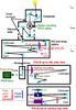 |
Fig. 1 Sketch of the light path at the VTT (drawing not to scale). Focal planes are denoted by blue rectangles, pupil planes by brown ones. Red rectangles denote an artificial blocking of the light path. The 45-deg mirror behind the relay optics was used to direct the light to either the PCO setup or towards POLIS. The design of POLIS is shown in side view up to the location of the slit (upper panel at lower right) and in top view for the rest of the optics (lower panel at lower right). |
2. Theoretical description of the stray-light problem
The transfer through the optical system composed of the (fluctuating) atmosphere of the
Earth, the telescope, and finally the instrument modifies the real intensity distribution
Itrue and yields instead an observed intensity
Iobs that is related to Itrue by
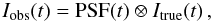 (1)where PSF(t) is the
instantaneous optical point spread function and ⊗ denotes a convolution.
(1)where PSF(t) is the
instantaneous optical point spread function and ⊗ denotes a convolution.
The three contributions to the PSF are explained in the introduction above. For observations with real-time correction by an AO system, the atmospheric part is already (partially) corrected for, leaving the large-scale atmospheric scattering and the static contributions from optics. The PSF spills the light from one location into its surroundings and vice versa, which adds additional intensity to all points in the FOV via false light originating in other locations in the FOV, the so-called stray-light contamination. To apply a correction for the stray-light contamination, we first derive a direct approach based on only the observed spectra and a generic estimate of the stray-light fraction in a simplified approach in the next section, and a more explicit model taking the instrumental PSF into account in Sect. 2.2.
2.1. Modeling of stray-light contributions
For the direct correction of the stray-light contamination, we model the intensity
spectrum Iobs(λ,x,y) on a certain CCD row in
the focal plane of the POLIS CCD cameras (focal plane F4, see Fig. 1) as  (2)with
 (3)where
“dc” denotes the dark current of the CCD.
Itrue(λ,x,y) is the spectrum that emerges
from the spatial location (x,y) on the Sun that corresponds to the CCD
pixel row y when the slit is located at position x on
the solar image. The average intensity spectrum before the first focal plane F1 is denoted
by Iglobal(λ); the full solar disk
contributes to it. Because of the CLV of the solar intensity,
Iglobal(λ) will be dominated by
contributions from the disk center and its surroundings, and its shape is independent of
the telescope pointing. This term corresponds to the integration over the full solar disk
weighted by a spread function, as done in, e.g., Mattig
(1971). It can be assumed that the stray-light level proportional to
Iglobal(λ) is uniform across the FOV, with
no direct relation to the solar location (x,y) where
Itrue(λ,x,y) originates. Scattering by any
of the optical elements in front of F1 will only need to produce slight beam deviations
from the optical axis to spill light from the full aperture to each location on the focal
plane because of the long path length before F1 is reached. The factor
α1 then refers to all nine optical elements in front of F1
(7 mirrors and 2 glass windows, see the upper part of Fig. 1).
(3)where
“dc” denotes the dark current of the CCD.
Itrue(λ,x,y) is the spectrum that emerges
from the spatial location (x,y) on the Sun that corresponds to the CCD
pixel row y when the slit is located at position x on
the solar image. The average intensity spectrum before the first focal plane F1 is denoted
by Iglobal(λ); the full solar disk
contributes to it. Because of the CLV of the solar intensity,
Iglobal(λ) will be dominated by
contributions from the disk center and its surroundings, and its shape is independent of
the telescope pointing. This term corresponds to the integration over the full solar disk
weighted by a spread function, as done in, e.g., Mattig
(1971). It can be assumed that the stray-light level proportional to
Iglobal(λ) is uniform across the FOV, with
no direct relation to the solar location (x,y) where
Itrue(λ,x,y) originates. Scattering by any
of the optical elements in front of F1 will only need to produce slight beam deviations
from the optical axis to spill light from the full aperture to each location on the focal
plane because of the long path length before F1 is reached. The factor
α1 then refers to all nine optical elements in front of F1
(7 mirrors and 2 glass windows, see the upper part of Fig. 1).
The average intensity spectrum behind F1,
Ilocal(λ), comes only from a restricted FOV
and not from the full solar disk because of the field stop in the filter wheel near F1.
The shape of Ilocal(λ) depends on the
telescope pointing. For the CLV observations, we used an aperture field stop with a
diameter of 40 mm (≈180′′). The diameter of the field stop in F2 inside of
POLIS is similar to the one of the field stop in F1. The stray light proportional to
Ilocal(λ) actually is made up of two
contributions: 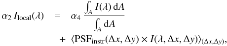 (4)where
A is the area of the field stop in F1, and
(Δx,Δy) the distance between (x,y)
and all other points inside the FOV that pass through the field stop.
(4)where
A is the area of the field stop in F1, and
(Δx,Δy) the distance between (x,y)
and all other points inside the FOV that pass through the field stop.
The first term is caused by the fact that the optical elements between F1 and F4 will uniformly mix the light across the full aperture of the field stop (as was the case for the optics upfront of F1), especially because there are three additional pupil planes in-between. The second term depends on the spatial PSF of POLIS that introduces a strongly field-dependent stray-light contribution to the spectrum from locations close to (x,y) when (Δx,Δy) is smaller than about 10′′ (see Sect. 3.4). PSFinstr only refers to the optics behind F1. We assume that both contributions on the right-hand side of Eq. (4) can be modeled as being proportional to the same profile Ilocal(λ) because in quiet Sun regions averaging over a small (a few arcsecs2) or large (several ten arcsecs2) area inside the local FOV will yield a similar profile. The factor α2 then refers to all optics between F1 and F4 (for POLIS: 15 mirrors, modulator, grating, interference filter, and the polarizing beam splitter for the 630 nm channel). The stray-light contributions proportional to Iglobal(λ) and Ilocal(λ) are both assumed to pass through a grating, and thus to be spectrally dispersed.
The “stray light” without wavelength dependence, the constant term in Eq. (2), again contains two contributions: the usual dark current (dc) of the CCD cameras and a second contribution that corresponds to light that reaches the CCD without passing through the grating, called “parasitic” light. The source of the parasitic light photons in the case of POLIS is indicated schematically in Fig. 2, which shows the optical design of POLIS just in front of the CCD cameras. In the light path behind the grating, a small pick-up mirror is used to deflect the blue part (indicated by a blue ray in the figure) of the dispersed spectrum towards the vertically mounted Ca ii H CCD camera (“blue channel”). The part of the spectrum at a longer wavelength (indicated in the figure by a red ray) instead passes below the pick-up mirror towards the channel at 630 nm (“red channel”). Spectrally undispersed scattered light inside the instrument (indicated in the figure by black arrows) can reach the 630 nm channel CCD only from a small solid angle, whereas most of the scattered light that hits the pick-up mirror can still reach the Ca ii H CCD at some place. Because the solar light level in the near-UV is rather low, especially in the line core of Ca ii H, additional photons can easily lead to a detector count rate that is significant with respect to the true solar spectrum.
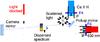 |
Fig. 2 Design of POLIS close to the CCD cameras in a side view (not to scale). “IF”: order selecting interference filters. The thin red rectangle indicates the location where the light path was blocked for measuring the parasitic stray light. |
The parasitic stray light is generated inside of POLIS. Its light level should therefore scale with the amount of light that enters through the field stop in F2, which can be related to the average of ⟨ Ilocal ⟩ . The coefficient α3 in Eq. (3) does not refer to any specific optical element.
Equation (2) can be simplified for any
practical application of a stray-light correction. The full aperture contributing to
Ilocal(λ) is rather large, covering more
than one supergranular cell and therefore providing a large-scale average profile similar
to a full-disk spectrum, and there are no means to determine
Iglobal(λ) from the observed spectra. We
thus substituted Iglobal(λ) with
Ilocal(λ), even if for observations off the
disk center there should be some difference between the two spectra because
Ilocal(λ) changes with the telescope
pointing. To apply the correction to observations, we here implicitly assume that the
average profile Ilocal(λ) is always
calculated from quiet Sun regions with a granular pattern. In the case of, e.g., sunspot
observations, this implies that only a subfield of the observed FOV is used for the
average. Because the dark current can be directly measured and subtracted, the simplified
version of Eq. (2) then reads as
 (5)Even
if the equation depends solely on two parameters, it turns out that determining
α is far from straightforward. In Sect. 3, we describe the results of our several different approaches to determine
α and β.
(5)Even
if the equation depends solely on two parameters, it turns out that determining
α is far from straightforward. In Sect. 3, we describe the results of our several different approaches to determine
α and β.
2.2. Stray-light correction and spatial deconvolution using a known PSF
To apply the stray-light correction, different approaches are possible. One straightforward method is based on the simplified Eq. (5). The knowledge of the instrumental PSFinstr also allows, however, more detailed methods to be used that take the spatial dependence of stray light – as given by the second term on the right-hand side of Eq. (4) – fully into account. For such approaches, we describe a first-order and a full correction by a deconvolution in the following.
2.2.1. First-order correction
To derive a first-order correction for the stray light caused by the instrumental PSF,
we reformulate and discretize Eq. (1) as
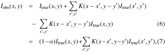 where
K is the kernel describing the instrumental PSF and the sums are to
be executed for all
x′,y′ ≠ x,y.
where
K is the kernel describing the instrumental PSF and the sums are to
be executed for all
x′,y′ ≠ x,y.
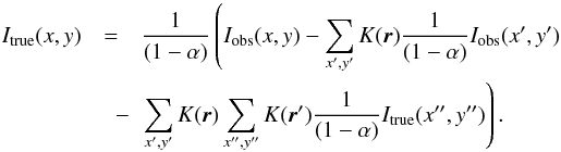
The last two terms on the right-hand side of Eq. (6) describe the stray light introduced into a location
(x,y) from other locations in the FOV (“gain” term) and the “loss” of
intensity to them, respectively. It can be shown that the first-order correction for the
gain term is given by  (8)when
all terms proportional to
α,α2,K α,K2
are neglected (see Appendix A). Equation (8) thus corresponds to the approach of
calculating the stray light that enters at (x,y) as the observed
intensity in the surroundings weighted by a PSF with a form as in the second term on the
right-hand side of Eq. (4).
(8)when
all terms proportional to
α,α2,K α,K2
are neglected (see Appendix A). Equation (8) thus corresponds to the approach of
calculating the stray light that enters at (x,y) as the observed
intensity in the surroundings weighted by a PSF with a form as in the second term on the
right-hand side of Eq. (4).
For an application of the correction, one has to take into account that for slit-spectrograph observations the scanning direction (denoted by x) and the direction along the slit (denoted by y) are not fully equivalent. All spectra Iobs(x′,y′) for x′ ≠ x are taken at a different time t′, and only the profiles in the individual spectrum Iobs(x,y′) are obtained simultaneously for all y′. Because the solar scene is changing with time during the scanning, it can therefore be necessary to restrict the sum in x′ to the temporally “close” surroundings instead of using the full range of the known PSF. The time lag between two scan steps is given by the integration time for each step tinteg times their distance Δx, where Δx·tinteg should be significantly smaller than the typical granular time scale of about five minutes.
The loss term in Eq. (7) could in principle be corrected for as well using the value of α, but given the difficulty of achieving high accuracy in its determination, that is not recommended. If the intensity normalization of the observed spectra is later done by normalizing an average profile after the correction to a theoretical or observed reference profile, the loss term will also be corrected for automatically by the normalization coefficient. The first-order correction is easy to apply and does not introduce numerical problems when K is given, despite some eventual interpolation in the construction of a discrete 2D kernel.
2.2.2. Fourier deconvolution
In the Fourier domain, Eq. (1)
transforms to  (9)where
 denotes the Fourier transform and only the static instrumental PSF described by the
kernel K is considered. It can be easily shown (e.g., DeForest et al. 2009) that for a known
K the reverse direction is given by
denotes the Fourier transform and only the static instrumental PSF described by the
kernel K is considered. It can be easily shown (e.g., DeForest et al. 2009) that for a known
K the reverse direction is given by  (10)where
 is the element-wise inverse operator for the Fourier transform of K.
The application of Eq. (10) exceeds the
first-order correction by taking both the gain and the loss term into account at the
same time. However, even if the derivation of
and the subsequent deconvolution is straightforward, its application can have unwanted
side effects, such as amplifying noise. We compared the Fourier transform of the inverse
PSF for POLIS with the corresponding Fig. 1 of DeForest
et al. (2009). The resulting curve directly resembled the kernel they obtained
after regularization for the noise suppression. For the present study
we therefore assumed that we do not need to additionally modify the PSF or apply a
high-frequency noise filtering before the deconvolution.
3. Stray-light measurements
The following sections describe the measurements for obtaining generic estimates of the stray-light level and of the instrumental PSF. We also suggest the best approach to applying the parasitic light correction.
3.1. Parasitic light
We start with the parasitic light coefficient β (Eq. (5)) because, unlike α, it can be determined directly. From the discussion of the source of the parasitic light in the previous section, it follows that if the direct illumination of the CCD with sunlight is blocked, only the randomly scattered light will be left over. This is thus the method of choice in determining β. We therefore compared measurements of a spectrum with a fully open aperture and a spectrum with the light path blocked close to the camera mirror inside of POLIS (Fig. 2). The location of the blocking prevented the direct illumination of the CCDs with the resolved spectrum, but did not affect the stray-light level inside the spectrograph otherwise. Both measurements were corrected for the dark current before the analysis.
To quantify the amount of parasitic light as a fraction of some mean intensity of the incoming light, we averaged the intensity of the full-aperture spectrum over a pseudo-continuum window in the spectrum from 396.383 nm to 396.393 nm as reference, and this yielded a mean value of 2716 counts. The average intensity value of the measurement without direct illumination of the CCD was around 148 detector counts. The corresponding image was homogeneously lit and showed no trace of spectral lines which ensures that no dispersed stray light was included in the measurement. The ratio of parasitic and reference intensity then is about 5% in the Ca ii H channel. The corresponding values for the channel at 630 nm were 20380 and 58 counts, respectively, yielding a fraction of 0.3% that is presumably negligible in an analysis of the 630 nm data.
For all following stray-light measurements in the Ca ii H channel, we have corrected the spectra for the parasitic light separately spectrum by spectrum. We determined the average intensity in the continuum window in each spectrum, averaging along the slit as well, and then subtracted 5% of this average value in detector counts from all intensity values of the spectrum.
 |
Fig. 3 Intensity normalization curve for the observations of 14/08/2009. The observed intensity at disk center is given by the black crosses, the red line is a polynomial fit to the data points. |
For the correction of scientific observations, we suggest using a slightly modified approach. From repeated small maps taken with about half an hour cadence at the center of the solar disk, one can obtain an intensity normalization curve for each point of time during the day. Figure 3 shows an example of such a curve for 14 August 2009. The first observation of this day was a large-area scan on disk center, so its intensity was used for the calibration curve, too. For each separate scan of a certain FOV, one then calculates the average profile over all scan steps, first dividing each spectrum by the corresponding value of the normalization curve. This removes the temporal trend during the scan and provides an average spectrum Ilocal with an intensity only proportional to that of the observed FOV. The parasitic correction is then given by the 5%-fraction of the intensity in the continuum window of the average profile. To include the change in light level during the observation again – because ⟨ Ilocal ⟩ at a given moment of time scales with it – the normalization curve from the start until the end of the scan is normalized to its mean value inside that time span. This provides the relative variation in the light level, hence of the parasitic correction for a spectrum taken at a given moment inside the FOV that entered into the calculation of Ilocal. Multiplying the parasitic correction with the relative temporal variation in intensity during the scan yields a correction for the parasitic stray light that accounts for both the variation in Ilocal with the telescope pointing and the temporal variation in the light level during the day.
3.2. Spider mounting
The guiding telescope of the VTT is fed by a small pick-up mirror located close to the entrance window of the evacuated telescope tube. The pick-up mirror is fixed to a spider mounting and produces a central obscuration in any pupil plane at the VTT. We set up an imaging channel to determine the light level inside the central obscuration. We deflected the light with the 45-deg mirror to an optical rail where we mounted a lens for creating a pupil image, a small-band interference filter at 557.6 nm, and some neutral density (ND) filters to reduce the intensity to a suitable level for the PCO Sensicam camera used. With this setup, we took images of the spider mounting in the pupil plane for a CLV run similar to the scientific observations, to measure the stray-light level and at the same time to identify a possible variation with the telescope pointing. The upper panel of Fig. 4 shows the resulting pupil images when moving across the solar disk in steps of 100′′. We took cuts through the images to determine the residual intensity in the shaded areas and normalized each of the cuts to its maximum intensity value (lower panel). The pupil images show a change in the global light level with the telescope pointing, but the intensity curves after the normalization are nearly identical. The residual intensity in the central obscuration is always about 4%. The light level at the border of the FOV (“tail”), which can only be caused by stray light, is below 2%. These numbers now, however, refer to a pupil plane, not a focal plane. After the reflection on the 45-deg mirror, the light passed through only three optical elements (lens, interference filter, ND filter). Because the spider mounting is located behind the entrance window, the stray light caused by the two coelostat mirrors and the entrance window is absent.
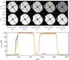 |
Fig. 4 Images of the pupil plane taken with the PCO setup in a CLV run at 557 nm. Top panel: pupil images, all shown in an identical display range. The offset of the telescope pointing from the disk center is given in each subpanel in arcsec. Bottom: intensities of each pupil image along the cut marked by the red vertical line in the image at 0′′. |
3.3. Methods without explicit measurements
There are three more methods that provide an estimate of stray light without requiring explicit measurements. The first is to match average observed spectra to an atlas profile, as suggested by Allende Prieto et al. (2004) and Cabrera Solana et al. (2007). A comparison with the presumably stray-light-free spectra of the FTS spectral atlas (Kurucz et al. 1984; Brault & Neckel 1987) yielded the best match for a value of β = 20% for both channels of POLIS. The approach is, however, not fully consistent with Eq. (5) because it implies that all stray light is of parasitic nature. Instead, the direct measurement of β of Sect. 3.1 excludes the high value retrieved with this approach. The approach is also aimed at determining the spectral point spread function of the optics behind the slit, because it uses an average observed profile without spatial resolution and the comparison of its shape to a reference profile. It therefore measures all spectral resolution effects of the spectrograph in addition to the parasitic contribution.
A second method is to compare profiles from the umbra of sunspots with only a little intrinsic radiation to an average quiet Sun spectrum. Rezaei et al. (2007) determined a level of at maximum 12% of stray light at 396 nm for the sum of α + β in the umbra, which can be taken as the minimum amount of stray light in the brighter quiet Sun surroundings. A simultaneous inversion of 630 nm and 1565 nm spectra with the SIR code yielded a value of α = 10% of stray light in the umbra (Beck 2006, 2008).
The last indirect method is the presence of residual polarization signal in the telluric line blends of the 630 nm channel. In the data reduction of long-integrated (>20 s) spectra of the 630 nm channel, the telluric lines at 630.20 nm and 630.27 nm sometimes showed a non-zero polarization signal even if the nearby continuum wavelengths showed none. This puzzling behavior could be traced back to the I → QUV cross-talk correction in combination with the real-time demodulation of the Stokes vector in POLIS. This demodulation uses pairs of image differences for Stokes QUV, but the addition of all images for Stokes I. Parasitic light thus adds up in I but cancels in QUV. For a correction of the cross-talk, one then has to use a reduced intensity Itrue = Iobs − const. in the calculation of the cross-talk coefficient cI → QUV = QUVobs/Itrue at continuum wavelengths. Subsequently, also cI → QUV·Itrue has to be subtracted from QUV. This additional correction was used in the data reduction of POLIS data in 2003 with const. ≡ β = 4% of Ic, but only for the long-integrated data. For shorter integration times, the effect was below the noise level and could not be detected. Because the stray-light covers in POLIS were modified afterwards as a consequence of this finding, the number can only serve as an order of magnitude estimate. We point out that this effect produces spurious polarization signals inside spectral lines caused by cross-talk from Stokes Ieven when close-by continuum wavelengths are forced to zero polarization.
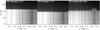 |
Fig. 5 POLIS Ca ii H spectra with partly illuminated FOV, logarithmic display range. Left: FOV blocked in F2 (hairline mounting). Middle: FOV blocked in F1 (filter wheel). Right: slit across the solar limb. |
3.4. FOV partially blocked in the focal plane (spatial PSF)
To derive the spatial PSF of POLIS, we took spectra with POLIS where part of the FOV in the focal plane was blocked by a metal plate. In addition to blocking part of the FOV in the focal planes F1 (telescope focus) and F2 (entrance of POLIS), we also took spectra with the slit placed across the solar limb. Figure 5 shows example spectra of the three cases. The blocking edge is sharper for the blocking in F2 inside of POLIS. This is caused by fewer optical elements being located behind F2, by the impossibility of using the adaptive optics while blocking in F1 and by the fact that the metal plate had to be placed at some distance to F1 (≈1 cm). All spectra are displayed on a logarithmic scale, otherwise the stray light could not be seen at all directly in the images. We then averaged the intensity in the same continuum window near 396.4 nm as before to obtain the spatial intensity variation across the blocking edge and the limb, respectively (Fig. 6).
To determine the spatial PSF, we then defined an artificial sharp edge located
appropriately along the slit, and constructed a model for the spatial PSF from a
combination of a Gaussian and a Lorentzian curve. We convolved the sharp-edge function
with the kernel and modified the free parameters of the two functions used in its
generation by trial-and-error until the convolved edge function (red line) matched the
observed intensity trend across the edge for the blocking in F1. The finally used kernel
is shown in the right part of Fig. 6 at about
x = + 25′′; it drops to basically zero at about
10′′ distance from its center. The area of the kernel is normalized to unity,
and its maximum value then is around 20%. For better visibility, it is shown multiplied by
four in the figure. The shape of the kernel can also be cross-checked against the observed
intensity variation by another method than the convolution of the sharp-edge function. In
case of an axisymmetric 2D kernel K(x,y), it can be
shown that the 1D kernel K(x) is given by
 (11)when the true intensity
corresponds to a step function and Iobs(x) is
the observed intensity variation across the step function (Collados & Vazquez 1987; Bonet et al.
1995).
(11)when the true intensity
corresponds to a step function and Iobs(x) is
the observed intensity variation across the step function (Collados & Vazquez 1987; Bonet et al.
1995).
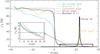 |
Fig. 6 Observed intensity variation along the slit for FOV blocked in F1 (black), blocked in F2 (green), and for the slit across the limb (blue). The purple lines at x,y = (0′′,100%) denote a simulated sharp edge that after convolution with the kernel at the right yields the red curve. The inlet on the left shows a magnification of the stray-light tail region. The derivative of the observed intensity variation for the FOV blocked in F1 is overplotted over the kernel as an orange line. |
We overplotted the derivative of the observed intensity variation for the blocking in F1 over the kernel in the right part of Fig. 6. The match is reasonably close, with a slightly lower central value and a broader central core in the derivative. The trial-and-error method for defining the kernel thus yielded a good match to the theoretical expectation.
Since the chosen kernel exhibits a sharp drop, most of the local stray light should come from the close vicinity (d < 2′′) of a given point (x,y). The inlet in the left-hand part of Fig. 6 shows that, actually, the tail level of the observations is not matched well, because the curve of the convolved sharp edge reaches zero several arc seconds before the observations. The residual intensity in the far tail (>20′′) is at maximum 2%. We point out that the observations of the solar limb and with the FOV blocked in F1 only differ slightly for x > 0′′, which implies that most of the stray light is caused by the instrumental PSF and not the telescope or atmospheric scattering.
For the application of Eqs. (8) and (10), a 2D kernel is needed. We used the
assumption of axial symmetry to create the 2D kernel K from the 1D
version shown in Fig. 6, and divided
K(x,y) by 2 π r,
with  ,
to maintain the normalization of the area of the 1D kernel.
,
to maintain the normalization of the area of the 1D kernel.
3.5. Summary of stray-light measurements
We used different methods to estimate the amount of stray light in POLIS. The upper two sections of Table 1 list the stray-light values determined in this work. In the lower section, we added the values that have been presented in previous studies for any of the two channels of POLIS. The definition of the stray-light fraction differs in most cases, but the umbral profiles provide a lower limit of 10–12% for the total stray-light contamination in quiet Sun areas without strong spatial intensity gradients. The parasitic light fraction could be accurately determined as 5% (0.3%) of the intensity for the channel at 396 nm (630 nm) for the data taken in 2009, but it presumably was higher in previous years before the modification of the stray-light covers inside the spectrograph. The stray-light level at distances above 20′′ from any lit area is on the order of 2% only, and the spatial PSF is strongly peaked with significant contributions only up to about 2′′. There were no indications that the relative stray light in the telescope changes somehow with the telescope pointing in a CLV run. The tail of the observed intensity variation across a sharp edge can be used as a proxy for the reduction of the stray-light level in off-limb spectra.
Stray-light levels for the VTT/POLIS in various studies.
4. Application to data
As a first application to observed data, we compare the performance of the stray-light corrections with and without explicitly using the instrumental PSF on a data set taken near the solar limb. The application to the limb data set actually yielded improved values for the stray-light contribution α because the residual intensity beyond the limb provides a good reference for the quality of the correction. In the second and third examples, we instead test the effects of the deconvolution as a method to improve the spatial resolution of observations on spectroscopic and spectropolarimetric data, respectively.
4.1. Example A: application to a limb data set
To test both the stray-light correction and the spatial deconvolution, we used a data set
that was taken near the solar limb on 25 August 2009, with an FOV that extended beyond the
limb (see Fig. 8 below). This offers a good
opportunity to determine the quality of the corrections because the limb is similar to a
sharp edge and beyond the limb the (pseudo-)continuum intensity should be zero. The map
was taken with 134 steps of 0 3 step width and
an integration time of 13 seconds per scan step (for more details see Beck & Rezaei 2011). We applied a variation of
corrections to the previously flat-fielded data to assess the effects of each step on the
data. We used the following combinations of corrections:
3 step width and
an integration time of 13 seconds per scan step (for more details see Beck & Rezaei 2011). We applied a variation of
corrections to the previously flat-fielded data to assess the effects of each step on the
data. We used the following combinations of corrections:
-
1.
parasitic light only (β);
-
2.
parasitic light (β) with subsequent first-order correction (Eq. (8));
-
3.
parasitic light (β) with subsequent Fourier deconvolution (Eq. (10));
-
4.
parasitic light (β) and stray light (α) as given by Eq. (5) (more details below).
Some of the approaches had to be modified slightly for treating off-limb spectra. Method No. 1 serves as a reference of basically uncorrected spectra. For the first-order correction in Method No. 2, we restricted the sum of Eq. (8) to (x′,y′) = (x,y) ± (5,40) pixels to avoid using scan steps that were taken at a significantly different time. The Fourier deconvolution in the 3rd method was done according to Eq. (10) by multiplying the Fourier transform of the 2D maps of the intensity at each wavelength, I(λ), with the inverse of the kernel.
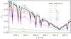 |
Fig. 7 Comparison of a large-scale average profile multiplied by α (thick black) and individual local stray-light profiles calculated around a given pixel using the PSF. The labels denote the distance of the pixel to the limb in arcsec (negative/positive ≡ on/off-disk). |
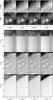 |
Fig. 8 2D maps and spectra after the correction. Lower panel: OW map in logarithmic display (bottom row), H2R map (middle row), spectra (top row) along the cuts marked by white vertical lines in the H2R map. Upper panel: magnification of the areas marked by black squares in the H2R map (on-disk and at the limb). The white rectangles denote the off-limb area used to derive the profiles of Fig. 10. |
For Method No. 4, we used a constant value of α = 10% as the minimum level of stray light for all spectra on the disk and an average local profile Ilocal calculated from the part of the FOV that was most remote from the limb. The intensity beyond the limb drops fast, however, with the limb distance (Fig. 6), so subtraction of a fixed α Ilocal yielded negative intensity values beyond the limb. To avoid this overcompensation, we scaled α down with increasing limb distance using the variation in intensity for the observation with the FOV blocked in F1 (Fig. 6). We took the observed intensity variation beyond the location of the edge (x < 0′′) and normalized the first point to 10% to have a smooth connection to the correction on the disk. The limb location was set to where the intensity dropped below 5% of Ic.
It turned out that a good off-limb correction was only achievable when the intensity of Ilocal was increased by a factor of two. Because the correction uses α Ilocal, the factor of two can be attributed either to αor Ilocal. Using an average disk center profile with its intrinsically higher intensity and keeping α at 10% yielded a worse result, because the spectral line blends in the wing were located at slightly different wavelengths than in the observed FOV, and it overcompensated for the stray light present as well. We therefore used an on-disk correction corresponding to α Ilocal with α = 20%, with the off-limb correction normalized to 20% on the first point.
The values used in the correction can actually be cross-checked with the PSF. Figure 7 shows α Ilocal used in Method No. 4 on the disk, together with some profiles corresponding to the gain term of Eq. (8), calculated locally from the surroundings of each pixel in the FOV weighted with the PSF. The stray-light contributions predicted by the gain term match the generic α Ilocal well, as long as the pixel, whose surroundings were used, was more remote from the limb than 10′′. The similarity of the stray-light profiles calculated using the PSF to each other and to the average profile supports using a single average profile Ilocal in Eq. (4) ignoring the PSF, but with a doubled α of 20%. The profile at 50′′ limb distance has a lower intensity because it is at the lower border of the FOV, where the full area of the kernel could not be used.
Figure 8 shows the result of applying all four methods (each shown in a column of the figure, in the same order as presented in the text) to the data set in 2D maps of the FOV and one sample spectrum. We derived one map in a pseudo-continuum window in the outer wing (OW, see, e.g., Beck et al. 2008) of the Ca ii H line and one map averaged over the wavelength region of the H2R emission peak. The amount of residual off-limb stray light can be clearly seen in the OW map (bottom row) and the spectra (third row). Only Method No. 4 removes the off-limb stray light satisfactorily.
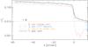 |
Fig. 9 Intensities across the limb in the OW wavelength range for an individual spectrum. Solid black line: Method No. 1. Triple-dot-dashed orange line: Method No. 2. Dash-dotted blue line: Method No. 3. Dotted red line: Method No. 4. |
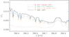 |
Fig. 10 Average off-limb spectra from the area marked by a white rectangle in Fig. 8. Line styles and colors are as in Fig. 9. |
The residual stray-light level beyond the limb is quantified in Fig. 9, which shows the intensity variation along the slit in the OW map for a randomly chosen scan step. The on-disk light level is globally reduced for Methods Nos. 2 and 4, whereas the Fourier deconvolution (No. 3) keeps the same level as the uncorrected spectra (No. 1). This reflects that only with the Fourier deconvolution is the loss term of Eq. (8) taken into account, whereas all other methods only correct the gain term. Beyond the limb, the stray-light level stays at the value of the uncorrected spectra of about 1–2% for the Fourier deconvolution (No. 3), whereas the first-order correction (No. 2) and the ad-hoc stray-light correction (No. 4) reduced the off-limb light level. The last method yields a correction an order of magnitude better than all others, reaching a level of about 0.2% of residual intensity.
The average profiles shown in Fig. 10, calculated for the off-limb area marked in the OW map of Fig. 8, also indicate the quality of the correction. These profiles allow instant differentiation of under/overcorrected stray light by the shape of the line blends in the wing: absorption profiles indicate residual stray light, whereas emission profiles for the photospheric blends at these heights above the limb indicate an overcorrection. Only Method No. 4 yields fully negligible residuals of the line blends. For the three other methods, absorption lines are seen in the wing. For the emission in the Ca ii H line core – basically, the only scientifically interesting quantity beyond the limb – Methods Nos. 2 and 4 yield a similar amplitude, whereas the Fourier deconvolution (No. 3) yields nearly the same intensity as the uncorrected spectra (No. 1).
Even if Method No. 4 gives the best results for the off-limb stray-light correction, this does not signify that the principle of the other methods is wrong. Methods Nos. 2 and 3 follow the initial way in which stray light is created closer than Method No. 4. Both approaches, however, only correct the static contribution to the stray light caused by the instrumental PSF, within the limits of accuracy in its derivation. Their worse performance beyond the solar limb implies that in this case both the residual dynamical part of the PSF beyond the AO correction and the PSF of the telescope and the optics upfront of F1 play a role. Because the true solar off-limb intensity outside of the very emission core is zero, any residual stray light not accounted for by the instrumental PSF is seen prominently in Figs. 8 or 10. The ad-hoc method (No. 4) instead seems to correct well for both the stray light caused by the instrumental PSF, as well as for the additional stray-light contributions, but only with a static correction without taking fluctuations of the atmospheric scattering into account.
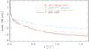 |
Fig. 11 Fourier power spectrum of the OW map vs. spatial frequency. Line styles and colors are as in Fig. 9. |
Spatial rms contrast and spectral rms noise in % of Ic.
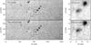 |
Fig. 12 Original (top row) and deconvolved (bottom row) continuum intensity maps at 777 nm of an active region with several pores. Left: full FOV. Right: magnification of the region marked by a black rectangle. |
As far as the spatial resolution is concerned, both the first-order correction (No. 2) and the Fourier deconvolution (No. 3) have led to an improvement, even if it is not very noticeable (second and third columns in the top two rows of Fig. 8). The Fourier deconvolution had a stronger effect on the visual impression. This is verified by the plot of the spatial Fourier power for the OW map shown in Fig. 11. Only the lower part of the OW map up to y = 40′′ was used. The power at higher spatial frequencies is slightly enhanced after the application of the first-order correction and significantly enhanced after the Fourier deconvolution. The improved spatial resolution is reflected also in the root-mean-square (rms) contrast of the OW maps (Table 2). This number, which measures the relative intensity variation, has, however, to be taken with caution because any correction that reduces globally the intensity automatically increases the rms contrast. We also determined the rms variation inside wavelength windows of about 10 pm extent in the OW spectral region and found it to stay basically at about 1.2% of Ic, with an average value of the intensity itself of about 20% at these wavelengths. The Fourier deconvolution (No. 3) has slightly increased the noise.
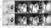 |
Fig. 13 2D maps of the sunspot observations at 630 nm. Top/bottom row: original/deconvolved spectra. Left to right: Stokes IQUV. The white dashed line marks the location of the cut shown in Fig. 14; the crosses and the corresponding numbers label the locations of the profiles shown in Fig. 15. The horizontal black/white lines at the upper and lower border of the FOV are caused by the hairlines of POLIS. |
4.2. Example B: application to pore observations at 777 nm
In another observing campaign in November 2009, we took identical measurements with a
partly blocked FOV with the main spectrograph of the VTT in a wavelength range around the
O i triplet at 777 nm. The corresponding convolution kernel derived from the
measurement is shown in Appendix B. The spatial
sampling along the 018 wide slit was
018 in this case.
We then applied the spatial deconvolution to an observation of an active region with
several pores, using Eq. (10) without any
additional stray-light correction. The spatial scanning in the observation was done with
201 steps of 036 width,
undersampling the slit width. Figure 12 shows the
full FOV before (upper left panel) and after the deconvolution (lower left panel). The
seeing was moderate to bad during the scan, producing frequent failures of the AO system,
with jumps of the FOV as well. The magnification of two of the pores (right panels),
however, shows that the deconvolution has not only increased the contrast by a reduction
of the intensity, but also leads to an improvement in the sharpness of the structures,
e.g., for the boundaries of the darkest parts of the pores.
4.3. Example C: application to polarimetric observations
To test the effect of the deconvolution by Eq. (10) on polarimetric data, we applied it to observations taken with POLIS in its
red channel at 630 nm. Assuming that the PSF derived for the blue channel is
characteristic of the instrument, we did not determine a new PSF but used the same one as
before. Appendix B shows that applying this kernel
to a knife-edge observation at 630 nm also provides a satisfactory match. The observation
we discuss here consists of a scan with 150 scan steps of
03 step width
across an active region (Fig. 13) done on 6 July
2005, with AO correction. The integration time was ten seconds per scan step. In this
case, the Fourier deconvolution was applied separately to each wavelength and Stokes
parameter.
In the visual impression of Fig. 13, the improvement in the spatial resolution is prominent, both in the continuum intensity map (left) and the maps of the absolute wavelength-integrated polarization signal, ∫|QUV|/Idλ. The umbral dots inside the umbra of the bigger spot can be seen well in the deconvolved data set and the filamentary structure of the penumbra of the smaller spot is much clearer. The rms contrast in the continuum image increased from 3.7% to 5.3%. Figure 14 demonstrates that the increase in the rms contrast is not only caused by the removal of the stray-light contamination. It shows a cut through the umbra of the larger sunspot where a light bridge was located. The full width at half maximum of the light bridge is slightly reduced and the intensity values to the left (x ~ 26′′) and right (x ~ 30.5′′) of the central region decrease to the benefit of a more concentrated distribution with a stronger intensity peak in the deconvolved data, compared to the original data.
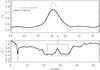 |
Fig. 14 Cut through the intensity maps of Fig. 13. Thick black: original data. Thin grey: deconvolved data. The upper panel shows a magnification of the central region where the cut crossed a light bridge. |
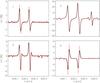 |
Fig. 15 Stokes V spectra from the sunspot observation. Red: deconvolved spectra. Black: original spectra. The numbers in the upper left of each panel refer to the labels in Fig. 13 that indicate the locations of the spectra in the 2D maps of the sunspot observation. |
The polarization signal was also usually amplified by the deconvolution. Figure 15 shows four Stokes V profiles before and after the deconvolution; taken from the locations marked in Fig. 13. On average, the Stokes V amplitudes increased relatively by about 5% of their previous value. These spectra, however, also clearly show the drawback of the Fourier deconvolution: the noise level is amplified as well. In Stokes I, the rms noise in a continuum window increased from 0.05% to 0.07% at an average value of about 15 000 counts. In Stokes V, where the noise level is more critical in the analysis of the data, the rms noise was 0.05% of Ic before and 0.12% of Ic after the deconvolution, respectively. The rms noise in Stokes V is still acceptable, even after the increase by a factor of 2.4. For comparison, Steiner et al. (2010) found an increase of the rms noise from 0.1% to 0.2–0.3% in the deconvolution of IMaX data.
5. The relation between PSF and (local) stray light
In the stray-light correction of the off-limb spectra, it turned out by trial-and-error that a value of α = 10% is definitely too low. The finally used stray-light level that yielded a good correction corresponds to using α = 20%. The integration of the local stray-light contribution using the PSF finally returned the same level (Fig. 7). As seen in Eq. (4), the PSF and the (local) stray light are mutually related to each other in a way that makes a separation between them difficult. To cross-check that the approach of using a single profile averaged over the full FOV instead of the explicit local version given by the PSF is reasonable, we calculated the local stray light using the gain term of Eq. (8) for all pixels of three data sets: the limb (@396 nm) and sunspot (@630 nm) observations used in the previous section, and a large-area map taken in quiet Sun (QS) on disk center (@396 nm, not shown here). We then determined the intensity of the local stray-light profiles relative to the average profile of the full FOV because the number can be used as first-order proxy1of the true α. Figure 16 shows the histograms of the relative frequency of occurrence of a given value of α. In QS regions, α is about 24%. For the limb and the sunspot data sets it is also generally at or above 20%; however, it can in some instances fall below 15% (see the tail of the corresponding distributions in the figure). Throughout the umbra of the large sunspot of Fig. 13, α was about 8–10%.
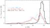 |
Fig. 16 Histograms of the local value of α in a QS map (thick black), a sunspot map (red), and the limb data set (thin blue). |
6. Discussion
The various stray-light measurements are basically consistent with the formulation of the stray-light problem in Eqs. (2), (4), and (6). For the special case of POLIS, the stray light contains a significant contribution of spectrally undispersed light created inside the instrument itself that could be absent in other spectrographs. For the spectrally resolved stray light that is created by scattering in the light path upfront of the grating, we found a lower limit of about 10% from umbral profiles and a value of about 20% in the quiet Sun, consistently from a limb data set and an application of the PSF to calculate the local stray light. A deconvolution with the instrumental PSF alone, however, does not provide a good correction for off-limb spectra, presumably because it only covers the optics behind the telescope focus and includes neither the atmospheric scattering nor the telescope PSF of the optics upstream of the focal plane. For off-limb data, additional corrections are needed that have eventually to be adjusted to the specific data set used, but a residual stray-light level below 0.5% can be achieved. For our data, we used the observed intensity variation across a sharp edge with only a minor ad-hoc adjustment to satisfactorily remove the off-limb stray light.
We determined the PSF from observations with a partly blocked FOV, for the two channels of POLIS and one observational run with the main spectrograph of the VTT at 777 nm. For the latter and the 630 nm channel of POLIS, the tail region of the stray light far away from the blocking edge was only partially reproduced, i.e., the derived kernel yields less stray light than actually observed. This is possibly related to our basically 1D approach using individual slit spectra. A spatial scan of the blocking edge and the determination of a 2D PSF may improve the result in the tail region because in the 1D case only the contamination along the slit is included, and not the “lateral” stray light. Determination of the instrumental PSF from observations with a half-blocked FOV is not limited to slit-spectrograph data but can equally be done for all kind of 1D or 2D instruments. It partly allows one to avoid having to use purely ad-hoc constructed PSFs as in Pereira et al. (2009), Joshi et al. (2011), or Rutten et al. (2011). The derivation of the PSF from explicit observations is more solid than the indirect method of a comparison between observed and synthetic spectra from simulations (e.g., Scharmer et al. 2011), where spatial and spectral resolution effects (cf. Sect. 3.3) can get mixed up.
The instrumental PSF can be used to deconvolve the observed spectra post-facto for both a correction of the stray light and an improvement of the spatial resolution. We tested the deconvolution on three different data sets, two spectroscopic and one spectropolarimetric observation. From the visual impression, the spatial resolution has improved in all cases beyond a simple increase in contrast owing to the global reduction of intensity because of the subtraction of the stray-light contribution. The noise level was increased by the deconvolution by up to a factor of about 2, while our PSF seems to be well behaved in general with respect to the noise amplification, presumably because it is sampling-limited in all cases and does not cover the high spatial frequencies down to the theoretically achievable diffraction limit where the noise contribution to the Fourier power also becomes important. For the polarimetric observation, we point out that we used the instrumental PSF to deconvolve an observation taken five years before the PSF measurement. Even if this still led to a clear improvement, the PSF measurement should be done closer in time. Before such a deconvolved data set can, however, be used for a scientific investigation, the effects of the deconvolution on the physically relevant quantities like the net circular polarization or the LOS velocities would have to be investigated in more detail (see, e.g., Puschmann & Beck 2011). This should include tests with synthetic observations that are convolved with the known PSF.
There are, however, more reasons that the deconvolution works well with the data sets used. The PSF is sharply peaked, therefore pixels with a separation of more than about 2–3′′ from a spatial location do not enter strongly. This automatically restricts the correction to the close surroundings of a given pixel, which is necessary for slit-spectrograph data with their sequential spatial scanning over a permanently evolving solar scene. A second reason is that all observations were obtained using AO correction, therefore the time-variant part of the instantaneous PSF is already largely compensated for. The third reason is that all observations initially have a high signal-to-noise (S/N) ratio because of the comparably long integration times of ten seconds or more. Finally, the observations were also spatially oversampled for the data used here; i.e., the spatial sampling along and perpendicular to the slit was below the effective resolution by a factor of two or more.
7. Conclusions
Observations with a partly blocked FOV in the first accessible focal plane allow one to estimate the (static) instrumental PSF downstream of the focal plane, in case no observations of a planetary transit are available, but it seems generally to be recommended to use a 2D FOV to determine the PSF. The PSF obtained allows one to determine the local stray-light contamination of a pixel from its close surroundings. For a homogeneously lit area – as is common in the quiet Sun – the explicit calculation by the PSF can be exchanged by an average stray-light contribution proportional to the average profile of the full FOV; in the case of sunspot observations, the stray-light correction should be calculated explicitly using the PSF because of the large intensity gradients. The PSF and the corresponding stray-light level can be cross-checked with observations near the solar limb, where continuum wavelength windows provide an excellent intensity reference. For ground-based observations taken with AO correction at the VTT, with a field stop before the first focal plane, the instrumental PSF seems to be dominating over the contributions from the telescope and the Earth’s atmosphere.
The PSF can also be used for a spatial deconvolution using a Fourier method. This seems a valid option for correcting slit-spectrograph observations post-facto for the static contributions of the instrumental PSF.
In Eq. (8), Iobs is used because Itrue is unknown; α is therefore slightly overestimated.
Acknowledgments
The VTT is operated by the Kiepenheuer-Institut für Sonnenphysik (KIS) at the Spanish Observatorio del Teide of the Instituto de Astrofísica de Canarias (IAC). The POLIS instrument has been a joint development of the High Altitude Observatory (Boulder, USA) and the KIS. C.B. acknowledges partial support by the Spanish Ministerio de Ciencia e Innovación through projects AYA 2007-63881, AYA 2010-18029, and JCI 2009-04504. D.F. gratefully acknowledges financial support by the European Commission through the SOLAIRE Network (MTRN-CT-2006-035484) and by the Programa de Acceso a Grandes Instalaciones Científicas financed by the Spanish Ministerio de Ciencia e Innovación. We thank C. Allende Prieto, B. Ruiz Cobo, M. Collados, and J. A. Bonet for helpful discussions. We thank the anonymous referee for providing helpful comments.
References
- Allende Prieto, C., Asplund, M., & Fabiani Bendicho, P. 2004, A&A, 423, 1109 [NASA ADS] [CrossRef] [EDP Sciences] [Google Scholar]
- Asplund, M., Grevesse, N., Sauval, A. J., & Scott, P. 2009, ARA&A, 47, 481 [NASA ADS] [CrossRef] [Google Scholar]
- Ballesteros, E., Collados, M., Bonet, J. A., et al. 1996, A&AS, 115, 353 [NASA ADS] [Google Scholar]
- Beck, C. 2006, Ph. D. Thesis, Univ. Freiburg [Google Scholar]
- Beck, C. 2008, A&A, 480, 825 [NASA ADS] [CrossRef] [EDP Sciences] [Google Scholar]
- Beck, C. A. R., & Rezaei, R. 2011, A&A, 531, A173 [NASA ADS] [CrossRef] [EDP Sciences] [Google Scholar]
- Beck, C., Schmidt, W., Kentischer, T., & Elmore, D. 2005, A&A, 437, 1159 [NASA ADS] [CrossRef] [EDP Sciences] [Google Scholar]
- Beck, C., Schmidt, W., Rezaei, R., & Rammacher, W. 2008, A&A, 479, 213 [NASA ADS] [CrossRef] [EDP Sciences] [Google Scholar]
- Beck, C., Bellot Rubio, L. R., Kentischer, T. J., Tritschler, A., & Del Toro Iniesta, J. C. 2010, A&A, 520, A115 [NASA ADS] [CrossRef] [EDP Sciences] [Google Scholar]
- Bonet, J. A., Sobotka, M., & Vazquez, M. 1995, A&A, 296, 241 [NASA ADS] [Google Scholar]
- Brault, J., & Neckel, H. 1987, Spectral Atlas of the Solar Absolute Disk-Averaged and Disk-Center Intensity from 3290 to 12 510 Å (unpublished, ditigal IDL version provided in the KIS sofware lib) [Google Scholar]
- Briand, C., Mattig, W., Ceppatelli, G., & Mainella, G. 2006, Sol. Phys., 234, 187 [NASA ADS] [CrossRef] [Google Scholar]
- Cabrera Solana, D., Bellot Rubio, L. R., Beck, C., & Del Toro Iniesta, J. C. 2007, A&A, 475, 1067 [NASA ADS] [CrossRef] [EDP Sciences] [Google Scholar]
- Cavallini, F. 2006, Sol. Phys., 236, 415 [NASA ADS] [CrossRef] [Google Scholar]
- Chae, J., Yun, H. S., Sakurai, T., & Ichimoto, K. 1998, Sol. Phys., 183, 229 [NASA ADS] [CrossRef] [Google Scholar]
- Collados, M., & Vazquez, M. 1987, A&A, 180, 223 [NASA ADS] [Google Scholar]
- DeForest, C. E., Martens, P. C. H., & Wills-Davey, M. J. 2009, ApJ, 690, 1264 [NASA ADS] [CrossRef] [Google Scholar]
- Fabbian, D., Khomenko, E., Moreno-Insertis, F., & Nordlund, Å. 2010, ApJ, 724, 1536 [NASA ADS] [CrossRef] [Google Scholar]
- Henoux, J. C. 1969, A&A, 2, 288 [NASA ADS] [Google Scholar]
- Joshi, J., Pietarila, A., Hirzberger, J., et al. 2011, ApJ, 734, L18 [NASA ADS] [CrossRef] [Google Scholar]
- Keller, C. U., & Johannesson, A. 1995, A&AS, 110, 565 [NASA ADS] [Google Scholar]
- Kneer, F., & Mattig, W. 1968, Sol. Phys., 5, 42 [NASA ADS] [CrossRef] [Google Scholar]
- Kurucz, R. L., Furenlid, I., Brault, J., & Testerman, L. 1984, Solar flux atlas from 296 to 1300 nm (National Solar Observatory, Sunspot, NM) [Google Scholar]
- Maltby, P. 1970, Sol. Phys., 13, 312 [NASA ADS] [CrossRef] [Google Scholar]
- Maltby, P., & Mykland, N. 1969, Sol. Phys., 8, 23 [NASA ADS] [CrossRef] [Google Scholar]
- MartinezPillet, V. 1992, Sol. Phys., 140, 207 [NASA ADS] [CrossRef] [Google Scholar]
- Mathew, S. K., Zakharov, V., & Solanki, S. K. 2009, A&A, 501, L19 [NASA ADS] [CrossRef] [EDP Sciences] [Google Scholar]
- Mattig, W. 1971, Sol. Phys., 18, 434 [NASA ADS] [CrossRef] [Google Scholar]
- Mattig, W. 1983, Sol. Phys., 87, 187 [NASA ADS] [CrossRef] [Google Scholar]
- Mikurda, K., Tritschler, A., & Schmidt, W. 2006, A&A, 454, 359 [NASA ADS] [CrossRef] [EDP Sciences] [Google Scholar]
- Orozco Suárez, D., Bellot Rubio, L. R., Del Toro Iniesta, J. C., et al. 2007a, PASJ, 59, 837 [Google Scholar]
- Orozco Suárez, D., Bellot Rubio, L. R., del Toro Iniesta, J. C., et al. 2007b, ApJ, 670, L61 [NASA ADS] [CrossRef] [Google Scholar]
- Pereira, T. M. D., Kiselman, D., & Asplund, M. 2009, A&A, 507, 417 [NASA ADS] [CrossRef] [EDP Sciences] [Google Scholar]
- Puschmann, K. G., & Beck, C. 2011, A&A, 533, A21 [NASA ADS] [CrossRef] [EDP Sciences] [Google Scholar]
- Puschmann, K. G., Kneer, F., Seelemann, T., & Wittmann, A. D. 2006, A&A, 451, 1151 [NASA ADS] [CrossRef] [EDP Sciences] [Google Scholar]
- Rezaei, R., Schlichenmaier, R., Beck, C. A. R., Bruls, J. H. M. J., & Schmidt, W. 2007, A&A, 466, 1131 [NASA ADS] [CrossRef] [EDP Sciences] [Google Scholar]
- Rimmele, T. R. 2004, in Advancements in Adaptive Optics, ed. D. Bonaccini Calia, B. L. Ellerbroek, & R. Ragazzoni, SPIE Conf. Ser., 5490, 34 [Google Scholar]
- Ruiz Cobo, B., & del Toro Iniesta, J. C. 1992, ApJ, 398, 375 [NASA ADS] [CrossRef] [Google Scholar]
- Rutten, R. J., Leenaarts, J., Rouppe van der Voort, L. H. M., et al. 2011, A&A, 531, A17 [NASA ADS] [CrossRef] [EDP Sciences] [Google Scholar]
- Scharmer, G. B., Dettori, P. M., Lofdahl, M. G., & Shand, M. 2003, in Innovative Telescopes and Instrumentation for Solar Astrophysics, ed. S. L. Keil, & S. V. Avakyan, SPIE Conf. Ser., 4853, 370 [Google Scholar]
- Scharmer, G. B., Narayan, G., Hillberg, T., et al. 2008, ApJ, 689, L69 [NASA ADS] [CrossRef] [Google Scholar]
- Scharmer, G. B., Löfdahl, M. G., van Werkhoven, T. I. M., & de La Cruz Rodriguez, J. 2010, A&A, 521, A68 [NASA ADS] [CrossRef] [EDP Sciences] [Google Scholar]
- Scharmer, G. B., Henriques, V. M. J., Kiselman, D., & de la Cruz Rodríguez, J. 2011, Science, 333, 316 [NASA ADS] [CrossRef] [Google Scholar]
- Schröter, E. H., Soltau, D., & Wiehr, E. 1985, Vist. Astron., 28, 519 [NASA ADS] [CrossRef] [Google Scholar]
- Staveland, L. 1970, Sol. Phys., 12, 328 [NASA ADS] [CrossRef] [Google Scholar]
- Steiner, O., Franz, M., Bello González, N., et al. 2010, ApJ, 723, L180 [NASA ADS] [CrossRef] [Google Scholar]
- Sütterlin, P., & Wiehr, E. 2000, Sol. Phys., 194, 35 [NASA ADS] [CrossRef] [Google Scholar]
- Tritschler, A., & Schmidt, W. 2002, A&A, 382, 1093 [NASA ADS] [CrossRef] [EDP Sciences] [Google Scholar]
- Tritschler, A., Schmidt, W., Langhans, K., & Kentischer, T. 2002, Sol. Phys., 211, 17 [NASA ADS] [CrossRef] [Google Scholar]
- van Noort, M., Rouppe van der Voort, L., & Löfdahl, M. G. 2005, Sol. Phys., 228, 191 [NASA ADS] [CrossRef] [Google Scholar]
- von der Lühe, O. 1993, A&A, 268, 374 [NASA ADS] [Google Scholar]
- von der Lühe, O., Soltau, D., Berkefeld, T., & Schelenz, T. 2003, in Innovative Telescopes and Instrumentation for Solar Astrophysics, ed. S. L. Keil, & S. V. Avakan, SPIE Conf. Ser., 4853, 187 [Google Scholar]
- Wedemeyer-Böhm, S. 2008, A&A, 487, 399 [NASA ADS] [CrossRef] [EDP Sciences] [Google Scholar]
- Wedemeyer-Böhm, S., & Rouppe van der Voort, L. 2009, A&A, 503, 225 [NASA ADS] [CrossRef] [EDP Sciences] [Google Scholar]
- Zwaan, C. 1965, Recherches Astronomiques de l’Observatoire d’Utrecht, 17 [Google Scholar]
Appendix A: Derivation of first-order correction
Solving Eq. (7) for
Itrue yields at first the recursive equation 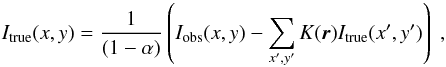 (A.1)where
r = (x − x′, y − y′).
(A.1)where
r = (x − x′, y − y′).
Exchanging the term
Itrue(x′,y′)
with the relation given by Eq. (A.1) gives
 (A.2)With
 for α ≪ 1 and
neglecting all terms
∝ α,α2,K α,K2,
one obtains
for α ≪ 1 and
neglecting all terms
∝ α,α2,K α,K2,
one obtains 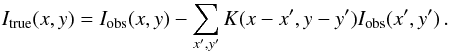 (A.3)
(A.3)
Appendix B: Convolution kernels at 777 nm and 630 nm
Convolution kernel at 777 nm.
Figure B.1 shows the observed intensity across the location of the blocking edge at 777 nm, together with the convolution kernel used to match the convolved edge function to the observation (upper panel). The kernel has more extended wings than the one of POLIS, but we were still not able to perfectly reproduce the tail region for distances over about 15′′ from the location of the edge (lower panel). Further increasing the wing contribution led to a mismatch on the other side of the edge in the lit area because the intensity of the convolved edge curve gets reduced more. Up to about 10′′ distance from the edge, the observations are reproduced well by the convolved edge.
 |
Fig. B.1 Derivation of the PSF at 777 nm. Thick black: observed intensity. Dashed: edge function. Thin red: convolved edge. Upper panel: observed intensity across the blocking edge. The convolution kernel is shown on the right; for better visibility it was multiplied by 2. Lower panel: “tail” region. |
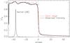 |
Fig. B.2 Test of the PSF at 630 nm. Thick black: observed intensity. Dashed: edge function. Thin red: convolved edge. The convolution kernel is shown on the left; it was multiplied by 8 for better visibility. |
Convolution kernel at 630 nm.
For the 630 nm channel of POLIS, we resampled the kernel determined at 396 nm to the two times finer spatial sampling in the red channel by interpolation. Figure B.2 shows that an application of this kernel to the edge function reproduces the intensity in the 630 nm channel for the observation with a half-blocked FOV satisfactorily, even if in the tail region the match is worse than for 396 nm. Because of the resampling, the amplitude of the kernel is halved compared to Fig. 6.
All Tables
All Figures
|
Fig. 1 Sketch of the light path at the VTT (drawing not to scale). Focal planes are denoted by blue rectangles, pupil planes by brown ones. Red rectangles denote an artificial blocking of the light path. The 45-deg mirror behind the relay optics was used to direct the light to either the PCO setup or towards POLIS. The design of POLIS is shown in side view up to the location of the slit (upper panel at lower right) and in top view for the rest of the optics (lower panel at lower right). |
| In the text | |
|
Fig. 2 Design of POLIS close to the CCD cameras in a side view (not to scale). “IF”: order selecting interference filters. The thin red rectangle indicates the location where the light path was blocked for measuring the parasitic stray light. |
| In the text | |
|
Fig. 3 Intensity normalization curve for the observations of 14/08/2009. The observed intensity at disk center is given by the black crosses, the red line is a polynomial fit to the data points. |
| In the text | |
|
Fig. 4 Images of the pupil plane taken with the PCO setup in a CLV run at 557 nm. Top panel: pupil images, all shown in an identical display range. The offset of the telescope pointing from the disk center is given in each subpanel in arcsec. Bottom: intensities of each pupil image along the cut marked by the red vertical line in the image at 0′′. |
| In the text | |
|
Fig. 5 POLIS Ca ii H spectra with partly illuminated FOV, logarithmic display range. Left: FOV blocked in F2 (hairline mounting). Middle: FOV blocked in F1 (filter wheel). Right: slit across the solar limb. |
| In the text | |
|
Fig. 6 Observed intensity variation along the slit for FOV blocked in F1 (black), blocked in F2 (green), and for the slit across the limb (blue). The purple lines at x,y = (0′′,100%) denote a simulated sharp edge that after convolution with the kernel at the right yields the red curve. The inlet on the left shows a magnification of the stray-light tail region. The derivative of the observed intensity variation for the FOV blocked in F1 is overplotted over the kernel as an orange line. |
| In the text | |
|
Fig. 7 Comparison of a large-scale average profile multiplied by α (thick black) and individual local stray-light profiles calculated around a given pixel using the PSF. The labels denote the distance of the pixel to the limb in arcsec (negative/positive ≡ on/off-disk). |
| In the text | |
|
Fig. 8 2D maps and spectra after the correction. Lower panel: OW map in logarithmic display (bottom row), H2R map (middle row), spectra (top row) along the cuts marked by white vertical lines in the H2R map. Upper panel: magnification of the areas marked by black squares in the H2R map (on-disk and at the limb). The white rectangles denote the off-limb area used to derive the profiles of Fig. 10. |
| In the text | |
|
Fig. 9 Intensities across the limb in the OW wavelength range for an individual spectrum. Solid black line: Method No. 1. Triple-dot-dashed orange line: Method No. 2. Dash-dotted blue line: Method No. 3. Dotted red line: Method No. 4. |
| In the text | |
|
Fig. 10 Average off-limb spectra from the area marked by a white rectangle in Fig. 8. Line styles and colors are as in Fig. 9. |
| In the text | |
|
Fig. 11 Fourier power spectrum of the OW map vs. spatial frequency. Line styles and colors are as in Fig. 9. |
| In the text | |
|
Fig. 12 Original (top row) and deconvolved (bottom row) continuum intensity maps at 777 nm of an active region with several pores. Left: full FOV. Right: magnification of the region marked by a black rectangle. |
| In the text | |
|
Fig. 13 2D maps of the sunspot observations at 630 nm. Top/bottom row: original/deconvolved spectra. Left to right: Stokes IQUV. The white dashed line marks the location of the cut shown in Fig. 14; the crosses and the corresponding numbers label the locations of the profiles shown in Fig. 15. The horizontal black/white lines at the upper and lower border of the FOV are caused by the hairlines of POLIS. |
| In the text | |
|
Fig. 14 Cut through the intensity maps of Fig. 13. Thick black: original data. Thin grey: deconvolved data. The upper panel shows a magnification of the central region where the cut crossed a light bridge. |
| In the text | |
|
Fig. 15 Stokes V spectra from the sunspot observation. Red: deconvolved spectra. Black: original spectra. The numbers in the upper left of each panel refer to the labels in Fig. 13 that indicate the locations of the spectra in the 2D maps of the sunspot observation. |
| In the text | |
|
Fig. 16 Histograms of the local value of α in a QS map (thick black), a sunspot map (red), and the limb data set (thin blue). |
| In the text | |
|
Fig. B.1 Derivation of the PSF at 777 nm. Thick black: observed intensity. Dashed: edge function. Thin red: convolved edge. Upper panel: observed intensity across the blocking edge. The convolution kernel is shown on the right; for better visibility it was multiplied by 2. Lower panel: “tail” region. |
| In the text | |
|
Fig. B.2 Test of the PSF at 630 nm. Thick black: observed intensity. Dashed: edge function. Thin red: convolved edge. The convolution kernel is shown on the left; it was multiplied by 8 for better visibility. |
| In the text | |
Current usage metrics show cumulative count of Article Views (full-text article views including HTML views, PDF and ePub downloads, according to the available data) and Abstracts Views on Vision4Press platform.
Data correspond to usage on the plateform after 2015. The current usage metrics is available 48-96 hours after online publication and is updated daily on week days.
Initial download of the metrics may take a while.