| Issue |
A&A
Volume 535, November 2011
|
|
|---|---|---|
| Article Number | A101 | |
| Number of page(s) | 7 | |
| Section | Stellar structure and evolution | |
| DOI | https://doi.org/10.1051/0004-6361/201015280 | |
| Published online | 18 November 2011 | |
Carbon isotopic abundance ratios in S-type stars⋆
1 Astronomy DepartmentUniversity of Washington, Seattle, WA 98195-1580, USA
e-mail: This email address is being protected from spambots. You need JavaScript enabled to view it.
; This email address is being protected from spambots. You need JavaScript enabled to view it.
2 Observatorio Astronómico Nacional, Apartado 1143, Alcalá de Henares, 28800 Madrid, Spain
e-mail: This email address is being protected from spambots. You need JavaScript enabled to view it.
; This email address is being protected from spambots. You need JavaScript enabled to view it.
3 Physical Sciences Dept., Everett Community College, Everett, WA, USA
e-mail: This email address is being protected from spambots. You need JavaScript enabled to view it.
Received: 24 June 2010
Accepted: 26 September 2011
Abstract
We have used the IRAM 30 m telescope on Pico de Veleta to observe 11 S-type stars in the J = 1–0 and J = 2–1 transitions of both 12C16O and 13C16O in order to derive the 12CO/13CO ratio in their circumstellar envelopes. Detections of high signal to noise were achieved for 7 stars. A mean isotope ratio of 35.3 ± 6.2 was found. This ratio fits between the ratio for late M stars of about 12 ± 3 and that of carbon stars of 58 ± 17. Hence, we confirm the often proposed evolutionary sequence from late M through type S to carbon stars. Mass loss rates of 5 × 10⁻⁸ to 3 × 10⁻⁶ M⊙ y-1 are derived from the present CO data using a simple uniform outflow model with line-dependent opacities, in very good agreement with previous mass-loss estimates.
Key words: stars: AGB and post-AGB / stars: abundances
Based on observations carried out with the IRAM 30 m radio-telescope. IRAM is supported by INSU/CNRS (France), MPG (Germany) and IGN (Spain).
© ESO, 2011
1. Introduction
Stars of type S were first recognized as a separate spectral class due to the presence of ZrO bands in addition to those of TiO in the spectra of cool giants (Merrill 1922). Merrill and others found that lines of many other heavy elements of the 4th and 5th rows of the periodic table are conspicuously enhanced in S stars. Merrill’s (1952) discovery of the unstable element technetium in S stars and its explanation by Cameron (1955) as a result of neutron captures by lighter species opened the way to the introduction of the s-process as defined and discussed by Burbidge et al. (1957).
For a full background on the evolution of asymptotic giant branch (AGB) stars see Worley et al. (2010, especially the contribution by A. Chieffi). As stars of about 1–8 M⊙ evolve beyond the first red giant branch their central regions convert 4He to 12C via the triple-alpha reaction. For sufficiently small masses, less than about 1.5 M⊙, He burning starts with a “flash” due to degeneracy and continues to convert helium to carbon quiescently. More massive stars, up to about 8 M⊙, burn He steadily in their cores. As the core becomes almost completely 12C (with some 16O in the most massive stars) the core shrinks and heats to the point at which the boundary between the 12C and the 4He can become active and shell burning can convert 4He to 12C. Due to the high temperature sensitivity of the 3-alpha reaction the rate rises very rapidly in what is called a “shell flash”. The large temperature gradient induces rapid convection which mixes the fresh 12C into higher layers. As the 12C is convected to the He-H boundary some of the 12C is converted to 13C by proton capture. This is the source of the 13C that is responsible for the free neutrons via the 13C(α, n)16O reaction. A wide range of elements including Zr are produced by successive neutron captures by Fe-peak elements. When further mixing brings these elements to the surface the atmospheric abundance of Zr is substantially enhanced and the star is called an S star.
Target stars.
During the mixing process, 12C is enhanced in the stellar atmosphere in which the ratio of 12CO/13CO had been depressed during previous CNO cycling. As atmospheric 12C is further enhanced in the upwelling of recently produced 12C the total carbon abundance equals, and then exceeds, the oxygen abundance and the atmosphere contains carbon molecules rather than oxides. That defines a carbon star. In a large survey of carbon stars, Lambert et al. (1986) found a range in 12C/13C from 20 to 90 with the exception of a few stars (known as J stars) with ratios near 3–4. Optical spectra of M giants by Luck & Lambert (1982) and Lambert & Smith (1990) have found 12C/13C ratios in the range of 7 to 23 with a mean of 15. This shows a small excess of 13C above the expected and observed ratio of 20 after the first dredge-up as a star evolves up the red giant branch for the first time. Similarly, in a survey of 18 additional M giants, mostly of types M4–M6, Brown and Wallerstein (unpublished) found a range of the 12C/13C isotope ratio of 8–18 with a mean of 12 ± 3.
This shows that most of the carbon that has been added to the atmosphere during stellar evolutionary phases that precede the formation of carbon stars, has been 12C. Yet available observations provide only sparse coverage in the gap from M giants to carbon stars. In this paper we endeavor to fill this gap with 12C/13C values measured in the molecular gas in the ejected envelopes of S stars.
It is difficult to derive the 12C/13C ratios from optical spectra of S stars, though some stars have been analyzed using the CN lines near 8000 Å and the CO lines in the near IR. In early M giants, there are CN bands near 8000 Å which show significant isotopic shifts, and carbon stars show both C2 and CN bands. For the cooler S stars, with which we are concerned here, the TiO, ZrO and LaO bands blend with the CN bands to make them essentially unusable.
It is necessary to use near IR or millimeter spectra where circumstellar CO transitions are observable in stars with envelopes formed by the stellar wind. The CO lines in the mm region are formed far out in the stellar envelope rather than in the photosphere where the optical and near-IR lines are formed. With modern technology, radio observations of 12CO and 13CO emission lines are becoming routine. Lines from 13CO are weaker than those from 12CO but generally detectable nonetheless. The 12CO lines are bright, though saturation can be an issue. In some cases, this can be avoided by using higher rotational transitions. Alternatively, radiative transfer in spherical winds can be used. We have pursued the latter course.
In this study, we have observed the CO isotopes with the IRAM 30-m telescope in the J = 1–0 and J = 2–1 transitions of 11 S stars as well as the calibration star CW Leo.
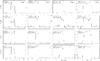 |
Fig. 1 Montage of CO spectra of S stars in which 13CO lines are visible. The main beam (observed) temperature, Tmb, is the ordinate in units of mK. 13CO and 12CO transitions are identified in the upper left corners of each panel along with the integrated line fluxes and the rms of Tmb. More saturated lines tend to exhibit flatter profile tops. Note that the relatively unsaturated 13CO lines invariably show double peaks. This is characteristic of uniform spherical expansion in a partially resolved envelope (see text). |
2. Target selection and observations
Targets were selected from an investigation of Li and Tc in Galactic S stars by Vanture et al. (2007), modified by the necessity that they be observable when the telescope was assigned to us. All of the stars show the Tc lines, demonstrating that they are intrinsic S stars rather than extrinsic S stars that have received heavy element-enhanced material from a now defunct companion. Possible exceptions are S Cas and W Aql, which we found to be too faint in the 4200 Å region in our search for Tc. S Cas has the longest period and one of the strongest Li lines among the S stars. Lambert et al. (1995) state that it is most likely an intrinsic S Star. With its period of 490 days and spectral type of S3, 9-S6, 9, W Aql is similar to S Cas. In Table 1 we show the most important properties of the observed stars. Useable trigonometric parallaxes are available for only 3 stars observed by Hipparcos (Van Leeuwen 2008). For all stars we list the derived MK magnitude using the period luminosity relation for Mira-type stars (Whitelock et al. 2008, Fig. 1), which has the form ![Mathematical equation: \begin{equation} M_K=\rho[{\rm log}~P-2.38]+\delta, \end{equation}](/articles/aa/full_html/2011/11/aa15280-10/aa15280-10-eq21.png) (1)where MK is the absolute K magnitude, P the pulsation period, and δ the zero-point of the MK–P relation, which has slope ρ.
(1)where MK is the absolute K magnitude, P the pulsation period, and δ the zero-point of the MK–P relation, which has slope ρ.
For non-Mira – i.e. semi-regular – variables we use the value suggested by Guandalini & Busso (2008), viz − 5.64 for MK. To estimate the distance, we accept the K magnitude as listed in SIMBAD, since the pulsation amplitude in K is not large. A comparison of the period-luminosity method with the HIPPARCOS parallaxes for 3 stars indicates that an uncertainty of about a factor of 2 is likely. Possible errors in distance have only a small impact on the derivation of the carbon isotope ratios.
The observations have been carried out with the IRAM 30 m millimeter radio-telescope (30 m-MRT), at an altitude of 2850 m located on Pico de Veleta (southern Spain). We have observed the two lowest rotational transitions, J = 2–1 and J = 1–0, of both 12C16O and 13C 16O isotopic substitutions of carbon monoxide (12CO and 13CO hereafter), at wavelengths of 2.6 and 1.3 mm. We have assumed rest frequencies of 110.201353 and 115.271202 GHz for the J = 1–0 line of 13CO and 12CO, and of 220.398681 and 230.537990 GHz for the J = 2–1 line of 13CO and 12CO, respectively.
The observations were performed in three runs, in June and November 2007, and in January 2009. During the first two runs, the weather conditions were mediocre to poor: precipitable water vapor content (PWV) from 1.0 to 10 mm, and total system noise equivalent temperatures (Tsys) of 100–300 K and 200–700 K at 2.6 and 1.3 mm respectively. On the contrary, weather was excellent on the last observing run, with PWV from < 0.5 to 2 mm and Tsys of 150–200 and 250–400 K at 2.6 and 1.3 mm respectively. The data presented here has been calibrated in units of (Rayleigh-Jeans-equivalent) main beam temperature (corrected for the atmospheric attenuation), Tmb, using the standard chopper wheel method. The temperature scale is set by observing hot and cold loads at ambient and liquid nitrogen temperatures. Correction for the antenna coupling to the sky and other losses have been applied using the latest values for these parameters measured at the telescope.
Finally, we accounted for the sky attenuation from the values of a weather station, the measurement of the sky emissivity and a numerical model for the atmosphere at Pico de Veleta. Calibration scans (observation of the hot and cold loads, and of the blank sky) were performed typically every 20 min. For the conversion into Tmb units, we have adopted values of the forward and main beam efficiencies of the telescope of 0.95 and 0.70, respectively, for the J = 1–0 lines, and of 0.91 and 0.58 for the J = 2–1 lines.
In addition to the method just described, during the runs we interspersed observations of strong (i.e. “template”) CO emitters to test the consistency of the calibration procedure. We believe that the final relative calibration between the different sources in our program is better than 10%, while the errors in the absolute calibration should be smaller than about 20%, after correcting for the variations observed in the strength of these CO template emitters.
The pointing of the telescope was checked, and corrected if necessary, when changing the observed source or every two hours, by cross-scan observations of strong continuum sources. From the results of the pointing scans we estimate that the overall pointing error during the observations is less than 2′′, which has negligible influence in the calibration even at the highest frequency observed. The observations were done by wobbling the secondary mirror by 2′ at a 0.5 Hz rate. This method provides very stable and flat spectral baselines, so after data averaging linear baselines have been fitted and subtracted from the final spectra.
At the telescope, we used the old A and B dual (3 and 1.3 mm) band receivers to observe simultaneously all four CO lines. In the last run, since we only observed 13CO, we recorded the two lines in two receivers at the same time, improving the S/N ratio by  after averaging. The receivers worked in SSB mode, with typical noise temperatures of 80 and 150 K at 2.6 and 1.3 mm respectively. As spectral back-end we used a 1 MHz resolution filter-bank for the 1.3 mm lines, and the VESPA auto-correlator in its 312.5 kHz resolution configuration for the J = 1–0 lines at 2.6 mm. This resulted in original spectral resolutions of 1.3 and 0.85 km s -1 for the J = 2–1 and J = 1–0 lines respectively.
In all cases, we observed just a single pointing towards the star position. The mean half-power beam width (HPBW) at the 30 m-MRT at 2.6 and 1.3 mm are 23′′ and 11.5′′ respectively. Depending on the relative extent of the CO envelope with respect to the main beam size of the telescope, a correction for the effect of the convolution of the molecular emission with the telescope beam has to be introduced. Corrections due to this effect mostly affect large envelopes in optically thick lines (J = 2–1 12CO) and can be estimated from the shape of all 4 CO lines.
3. Results
Opacity effects in the radiation transfer of the 12CO and, to a smaller degree, the 13CO lines force the use of a model to interpret the observational data. The double-horned profile shapes that characterize the 13CO and the likelihood of steady mass loss in S stars motivate the use of a uniformly expanding spherical model for estimating mass loss rates and 12CO/13CO abundance ratios from our observations. Fortunately, as we will see, our method is simple and robust thanks to the favorable properties of the excitation and emission of the CO low-J transitions.
We follow the theoretical intensity predictions by Knapp & Morris (1985). These authors performed grids of calculations that give values of the 12CO J = 1–0 intensity for values of the mass-loss rate, Ṁ, the distance D to the star, the CO abundance X(CO) relative to H2 (assumed to be 6 × 10⁻⁴), the circumstellar expansion velocity, Vexp, and the outer radius of the CO-rich envelope, RCO, beyond which the CO dissociates.
In general, the excitation and emission of low-J CO lines is very easy to describe physically, due to the simple level structure of this molecule and that the populations of all of the low-lying levels are thermalized even for relatively low densities. For example, the J = 1–0 transition requires an excitation temperature of only 5.5 K, to be excited. Thus, for simplicity, we will base our estimates on observations of this line.
Another advantage of using J = 1–0 profiles is that the extended CO envelope is rarely larger than our telescope beam, ~ 23′′ at 115 GHz. As we will explain below, we have applied corrections to the line intensities for the few sources that may be partially resolved, in order to introduce the resulting intensities in the estimates of the mass-loss rates from the theoretical grids. In any case, those corrections are almost always very modest and their uncertainty has little effect on our results.
In most cases, the parabolic shapes and in general central peaks in the 12CO profiles are a clear sign of a significant degree of opacity in the expanding envelope (see general discussion by Olofsson et al. 1982), which must be taken into account in the calcultions. Since it is possible that 12CO/13CO < 10, opacity effects for 13CO profiles cannot be dismissed. However, for those profiles with two horns or oddly shaped profile cores – as in most of our 13CO profiles – we can assume optically thin lines. These general trends have been widely confirmed by observations and theoretical detailed models (see e.g. Ramstedt et al. 2008; Teyssier et al. 2006).
In Fig. 1 we present examples of our 12CO and 13CO profile shapes. Four stars in our survey show signs of optically thick 12CO emission: W Aql, R And, S Cas, and R Cyg. Of these, high opacity is confirmed in W Aql and S Cas (Ramstedt et al. 2009; Nyman et al. 1992). So we will apply the full optically thick case for them. For R And and R Cyg, in which the opaque nature of the lines is less clear, we will adopt values averaged between those obtained from the optically thin and thick cases. As discussed in Appendix A, the estimated 12CO/13CO abundance ratios are in fact not very different in both cases.
For optically thick lines, the comparison of the observed line profiles with the models we use to estimate mass-loss rates requires an estimate of the profile’s central temperature of the J = 1–0 lines for a beam that includes the entire CO outflow zone. For relatively small sources, these values are directly given by our observations. In some cases, in which the shell is partially resolved, some correction must be applied. Such corrections are estimated assuming that all the emission at velocities well separated from the systemic one is well picked up by our single-point observations, since at these velocities the line emission comes from an angularly compact region along the central line of sight that can be assumed to be always unresolved. The peak intensity was then estimated by applying to our observations the relative increase between the central peak and the adjacent velocities found in the profiles of our targets obtained by Ramstedt et al. (2009) and Nyman et al. (1992), who used a wider beam. Even so, the procedure is a bit risky for W Aql and S Cas owing to possible uncertainties in our respective intensity calibrations.
This problem is less important in optically thin cases, in which the line peak always appears at extreme velocities, leading in the limit to clear two-horn profiles. We recall that the brightness distribution at those extreme velocities, which comes from an angularly compact region along the central line of sight, can be assumed to be unresolved. Therefore, our peak intensities should accurately give the intensity measure needed to be included in the theoretical estimates.
We note that the expected outer CO radii adopted by Knapp & Morris (1985), as due to CO photodissocition, are now understood to be too large owing to new better studies of dissociation by the interstellar UV radiation field. Detailed calculations of the CO photodissociation radius were performed by Mamon et al. (1988) for the relevant cases, taking into account the shielding by dust and by the CO molecule itself. The resulting predicted radii were parameterized as a function of the mass loss rate, the expansion velocity, and the relative abundance by Planesas et al. (1990), see also Loup et al. (1993). Accordingly, we introduced the photodissociation radius calculated in this way in the grids by Knapp & Morris, in our calculation of mass-loss rates and 12CO/13CO abundances. Since the radius also depends on Ṁ and distance, the procedure needs to be applied iteratively.
We note that the outer 13CO radius is practically identical to that of 12CO (Mamon et al. 1988) because, although 13CO is more easily photodissociated by the interstellar UV field, subsequent fractionation reactions tend to reform 13CO. To first order, the abundance is kept practically constant up to the photodissociation radius of 12CO. From this radius, both molecules are dissociated and their abundances drop very fast.
13CO J = 1–0 is always found to be optically thin in our targets, as expected for the typical low abundance of this species in circumstellar envelopes around AGB stars. However, we note that opacity corrections could also be applicable to 13CO emission in a few extreme cases of small 12CO/13CO values, since the excitation of both isotopic substitutions is very similar. In the unrealistic case where 12CO ≈ 13CO the predicted intensities of their J = 1–0 lines are the same aside from a small difference ≈ (115 GHz/110 GHz) 2, ~ 9%. In the more general case where 12CO/13CO > 10, this type of uncertainty is significantly smaller than the general uncertainty in the theoretical analysis of CO data. Thus, we have not tried to introduce any correction when applying the theoretical grids to 13CO.
Finally, we note that the value of X(12CO) has been very well studied in circumstellar envelopes. But even if X(12CO) is somehow unique for S stars, the adopted value is not critical in our estimates of the 12CO/13CO abundance, because any change in X(13CO) affects the determination of Ṁ yielding a change in X(12CO) in the same sense.
In summary, using the above procedure, we have first estimated the mass-loss rate and the CO photodissociation radius from our 12CO J = 1–0 profiles. We then used these results to estimate the abundance of 13CO and therefore the 12CO/13CO relative abundance.
Typical CO spectra for χ Cyg, R And, R Cyg, and S Cas are shown in Fig. 1. For T Sgr and the short period stars T Cet, AA Cam, and TV Aur, the S/N was insufficient to derive useful isotope ratios. The peak line intensities as well as the mass loss rates and CO isotopic ratios derived from these spectra are shown in Table 2. Obviously the 13CO lines are partially saturated in some of the target stars. The final column of Table 2 shows how we treated these lines in the model analysis. In two cases, it is not clear if the lines are predominantly optically thick or thin, so we performed two calculations and adopted the average values. The mass-loss estimates are from our data and our simple modeling (based on the calculation grids by Knapp & Morris 1985), and derived 12CO/13CO abundance ratios.
Peak line intensities and other parameters derived from our observations.
Based on the 5 Miras and 2 semi-regular variables for which measurements are feasible, the mean isotopic ratio of 12C/13C is 36.1 after correction for opacity effects. The dispersion in 12C/13C is 7.5 with extreme values between ~ 25 and ~ 46 for objects in which both lines were detected. The mean isotopic abundance for our sample is close to the geometric mean for M and carbon stars, suggesting the S stars fill the gap along the AGB between M and carbon stars.
Velocity measurements (ordered by pulsation period).
In Table 3 we show the full width at half maximum (FWHM) of the strongest CO feature, the central velocity, the previously measured optical velocity, and the source for the latter. All velocities are heliocentric in km s-1. Optical data are taken from SIMBAD, most of which come from the General Catalogue of Radial Velocities (Wilson 1953) and are usually based on the high-dispersion spectra obtained by P. W. Merrill with the Mt. Wilson spectrographs. These observations were based on spectra in the 4000–5000 Å region where the atmospheric opacity is high due to Rayleigh scattering by the H2 molecule. Thus, they represent the radial velocity at the upper layer of the atmosphere.
Comparison of mass loss estimates (M⊙ yr-1).
In Table 4 we show the estimated mass loss rates based on (1) sophisticated model fitting by Ramstedt et al. (2009) and (2) from our simple estimates. For our estimates we have adopted the same stellar parameters as Ramstedt et al. wherever possible. For some stars, we present calculations in both optically thin and thick cases. In some cases, when none of the values appear between brackets, it is not clear if the emission is optically thin or thick and the best estimate is an average of both. The asterisks indicate the stars in which we could not use 1–0 data from Ramstedt et al., and so the ratio between the estimates is affected by calibration uncertainties. The agreement of both methods is very satisfactory.
There is a noticeable correlation between the envelope expansion velocity and period that has long been known for Mira stars. We have also compared the CO and optical velocities. We find a systematic difference of 6.2 ± 2.4 km s-1 for six regular Miras. In contrast, the difference is 1.75 ± 1.0 km s-1 for the four semi-regulars. Both sets of differences are in the sense that velocities from spectra in the blue region are larger. Our difference of 6.2 km s-1 for the six Miras is almost the same as the K term of 5 km s-1 derived by Reid (1976).
The agreement is limited by uncertainties in the outflow speeds at the stellar surface where the optical lines arise and the cooler envelope outflow in which the molecular lines are formed and excited. That is, Mira atmospheres are dynamic in which rising and falling parcels of gas form radiative shocks during portions of the pulsation cycle (Hinkle et al. 1982).
4. Discussion
The S stars appear to be in an evolutionary stage on the asymptotic giant branch between the M giants and the carbon stars. During their evolution, 12C produced in shell flashes is convected to the surface and the abundances of various heavy elements are enhanced by neutron captures. The neutrons are released by the reaction 13C(α, n)16O which serves also to deplete the 13C (Herwig, 2005; Palmerini et al. 2009). In late M giants, the 12C/13C ratio is about 12 ± 3 (Luck & Lambert 1982; Smith & Lambert 1990a,b; Wallerstein & Morell 1994; Brown & Wallerstein, unpublished). For carbon stars, excluding the CH stars and the J-type subspecies, the 12C/13C ratio ranges from 20 to 90 with a mean of 58 ± 17 (Lambert et al. 1986). Thus, the 12C/13C ratio of S stars fits nicely between that of late M giants and carbon stars, as is expected from the evolutionary sequence that has long been hypothesized.
In addition to the carbon isotopes, there are several features in the spectra of S stars that are sensitive to nuclear reactions in the stars themselves, as noted in Table 1. These are the presence and strength of the resonance line of Li, the strength of the Zr lines and ZrO bands, and the presence of the Tc I lines. Each of these is affected by reactions in the stellar interior and mixing to the surface. Even if Tc is produced and mixed to the surface, its presence limits the time since its production to a few half-lives or less than a million years.
7Li is produced in red giants by the Cameron-Fowler (1971) process whereby 4He + 3He → 7Be, which decays to 7Li with a half-life of 53 days. It must be convected to lower temperatures before decaying or else the 7Li is converted to two 4He nuclei by proton capture. The 12C/13C ratio is strongly affected by proton capture by 12C but the 13C may capture another proton to make 14N. At temperatures near 108 K, neutrons are released by 13C(α, n)16O and are available to produce heavy elements such as the Sr, Y, Zr group as well as Ba and the lighter rare earths. This process is undoubtedly the source of the excess Zr and the Tc seen in S stars (Cameron 1955). In Table 1 we have shown the presence of each of these key species in our target stars.
Lithium appears in some galactic S stars (Vanture et al. 2007) as well as in S stars in the Magellanic Clouds (hereafter MC) (Smith & Lambert 1989, 1990a,b; Plez et al. 1993). This discovery was a surprise as lithium is easily destroyed at the temperatures necessary to synthesize Tc and other post-iron peak elements via the s-process. The presence of Li in the S stars of the MC is nicely explained by the process of Hot Bottom Burning (HBB) (D’ Antona & Mazzitelli 1996; Mazzitelli et al. 1999; Sackmann & Boothroyd 1992; Boothroyd et al. 1993). In HBB, 7Li is produced in red giants by the Cameron-Fowler mechanism (Cameron & Fowler 1971). The HBB theory makes specific predictions about the 12C/13C ratio in the photospheres of Li-rich AGB stars, namely the ratio should be low between 3 and 18 (Boothroyd et al. 1993).
There are three stars in our sample that exhibit both Tc and Li lines in their spectra, TV Aur, R Cyg and T Sgr (Vanture et al. 2007). A fourth star, S Cas, has a strong Li resonance line (Vanture et al. 2007; Lambert et al. 1995). Though no determination of the presence of Tc lines in the spectrum of S Cas exists in the literature, Lambert et al. (1995) argue that it is most likely an intrinsic S star based upon characteristics that it shares with other known intrinsic S stars. Therefore, it is expected that S Cas will exhibit Tc lines in its spectrum. The lithium line in S Cas is very strong (Lambert et al. 1995) and a comparison of its appearance as illustrated in Fig. 2 of Vanture et al. (2007) to that in the super-Li rich S star V441 Cyg as shown in Fig. 7 of Uttenthaler & Lebzelter (2010) suggests that S Cas may also be a super-Li S star. The Li abundance of V441 Cyg (log ϵ(Li) = 4.4; Uttenthaler & Lebzelter 2010) as well as that of T Sgr (log ϵ(Li) = 4.2; Abia et al. 1991), on the abundance scale of log ϵ(H) = 12.0, are in agreement with the predictions of HBB.
Of the four stars in our sample which can be classified as intrinsic S stars with enhanced Li abundances the lower limit of the 12C/13C ratio of TV Aur and T Sgr do not conflict with the predictions of HBB. However, the carbon isotope ratios in S Cas and R Cyg are well above those predicted by HBB theory. If R Cyg and S Cas have lithium abundances comparable to those of V441 Cyg and T Sgr (and the evidence that this is true for S Cas at least is compelling) then our results present a problem for HBB theory.
In addition, HBB theory predicts that these stars should have Mbol < − 6.0 and the bolometric magnitudes predicted using Eq. (1) are well above this limit for the four stars with Li. However, it should be noted that predicting the Mbol of Galactic S stars is not an exact science. For example, Uttenthaler & Lebzelter (2010) give Mbol for V441 Cyg of − 5.7, while using Eq. (1) we would determine a value of − 4.45. If this offset were uniform and the scale of Uttenthaler & Lebzelter (2010) is correct, then R Cyg, T Sgr and S Cas would have bolometric magntidues of approximately − 6.0, though TV Aur would still be one magnitude above this limit.
There are other super-Li rich stars, notably WZ Cas, that present difficulties for HBB theory. Abia et al. (1999) find that WZ Cas (a star on the SC-C border) has log ϵ(Li) ≥ 3.0 and 12C/13C of 5. However, HBB theory predicts that there should be no super-Li rich carbon stars (Boothroyd et al. 1993). Domínquez et al. (2004) find a super-Li rich carbon star in the Draco dwarf galaxy with 12C/13C > 40. In fact, García-Hernández et al. (2007) argue that there should not be any super-Li rich S stars formed by HBB in the Milky Way. A cool bottom burning process (CBP) has been proposed by Wasserburg et al. (1995) to explain abnormal Li abundances among RGB and low mass AGB stars. However, CBP predicts low values of 12C/13C as well which is at odds with the findings of García-Hernández et al. (2007) and our findings for S Cas and R Cyg.
Acknowledgments
We thank the outstanding staff at the Pico Veleta Radio Observatory which is operated by the Institut de Radio Astronomy Millimetrique, Grenoble. We also thank A. Ritchey for help in preparing this paper for publication. B. Balick acknowledges the support from grant AST 0808201 from the National Science Foundation. Andrew Vanture’s summer research has been supported by the Kenilworth Fund of the New York Community Trust. This work is partially supported by the Spanish MICINN, program CONSOLIDER INGENIO 2010, grant “ASTROMOL” (CSD2009-00038).
References
- Abia, C., Boffin, H. M. J., Isern, J., & Rebolo, R. 1991, A&A, 245, L1 [NASA ADS] [Google Scholar]
- Abia, C., Pavlenko, Y., & de Laverny, P. 1999, A&A, 351, 273 [NASA ADS] [Google Scholar]
- Ake, T. B. 1979, ApJ, 234, 538 [NASA ADS] [CrossRef] [Google Scholar]
- Burbidge, E. M., Burbidge, G. R., Fowler, W. A., & Hoyle, F. 1957, Rev. Mod. Phys., 29, 547 [NASA ADS] [CrossRef] [Google Scholar]
- Boothroyd, A. I., Sackmann, I. J., & Ahrens, S. C. 1993, ApJ, 416, 762 [NASA ADS] [CrossRef] [Google Scholar]
- Cameron, A. G. W. 1955, ApJ, 121, 144 [NASA ADS] [CrossRef] [Google Scholar]
- Cameron, A. G. W., & Fowler, W. A. 1971, ApJ, 164, 111 [Google Scholar]
- D’Antona, F., & Mazzitelli, I. 1996, ApJ, 470, 1093 [NASA ADS] [CrossRef] [Google Scholar]
- Domíguez, I., Abia, C., Straniero, O., Cristallo, S., & Pavlenko, Y. 2004, A&A, 422, 1045 [NASA ADS] [CrossRef] [EDP Sciences] [Google Scholar]
- Famaey, B., Jorissen, A., Luri, X., et al. 2005, A&A, 430, 165 [NASA ADS] [CrossRef] [EDP Sciences] [Google Scholar]
- Feast, M. W., Woolley, R., & Yilmaz, N. 1972, MNRAS, 158, 23 [NASA ADS] [CrossRef] [Google Scholar]
- García-Hernández, P. A., García-Lario, P., Plez, B., et al. 2007, A&A, 462, 711 [NASA ADS] [CrossRef] [EDP Sciences] [Google Scholar]
- Groenewegen, M. A. T., van der Veen, W. E. C. J., & Matthews, H. E. 1998, A&A, 338, 491 [NASA ADS] [Google Scholar]
- Herwig, F. 2005, ARA&A, 43, 435 [NASA ADS] [CrossRef] [Google Scholar]
- Hinkle, K. H., Hall, D. N. B., & Ridgway, S. T. 1982, ApJ, 252, 697 [NASA ADS] [CrossRef] [Google Scholar]
- Keenan, P. C. 1954, ApJ, 120, 484 [NASA ADS] [CrossRef] [Google Scholar]
- Keenan, P. C., & Boeshaar, P. C. 1980, ApJS, 43, 379 [NASA ADS] [CrossRef] [EDP Sciences] [Google Scholar]
- Knapp, G. R., & Morris, M. 1985, ApJ, 292, 640 [NASA ADS] [CrossRef] [Google Scholar]
- Lambert, D. L., Gustafsson, B., Eriksson, K., & Hinkle, K. H. 1986, ApJS, 62, 373 [NASA ADS] [CrossRef] [Google Scholar]
- Lambert, D. L., Smith, V. V., Busso, O., Gallino, R., & Stranerio, O. 1995, ApJ, 450, 320 [Google Scholar]
- Loup, C., Forveille, T., Omont, A., & Paul, J. F. 1993, A&AS, 99, 291 [NASA ADS] [Google Scholar]
- Luck, R. E., & Lambert, D. L. 1982, ApJ, 256, 189 [NASA ADS] [CrossRef] [Google Scholar]
- Mamon, G. A., Glassgold, A. E., & Huggins, P. J. 1988, ApJ, 328, 797 [NASA ADS] [CrossRef] [Google Scholar]
- Mazzitelli, I., D’Antona, F., & Ventura, P. 1999, A&A, 348, 846 [NASA ADS] [Google Scholar]
- Merrill, P. W. 1922, ApJ, 56, 475 [NASA ADS] [CrossRef] [Google Scholar]
- Merrill, P. W. 1952, Science, 115, 484 [Google Scholar]
- Nyman, L.-A., Booth, R. S., & Carlstrom, U. 1992, A&AS, 93, 121 [NASA ADS] [Google Scholar]
- Olofsson, H., Johansson, L. E. B., Hjalmarson, A., & Nguyen-Quang-Rieu 1982, A&A, 107, 128 [NASA ADS] [Google Scholar]
- Palmerini, S., Busso, M., Maiorca, E., & Guandalini, R. 2009, PASA, 26, 161 [NASA ADS] [CrossRef] [Google Scholar]
- Planesas, P., Bachiller, R., Martín-Pintado, J., & Bujarrabal, V. 1990, ApJ, 351, 263 [NASA ADS] [CrossRef] [Google Scholar]
- Plez, B., Smith, V. V., & Lambert, D. L. 1993, ApJ, 418, 812 [NASA ADS] [CrossRef] [Google Scholar]
- Ramstedt, S., Schöier, F. L., Olofsson, H., & Lundgren, A. A. 2008, A&A, 487, 645 [NASA ADS] [CrossRef] [EDP Sciences] [Google Scholar]
- Ramstedt, S., Schöier, F. L., & Olofsson, H. 2009, A&A, 499, 515 [NASA ADS] [CrossRef] [EDP Sciences] [Google Scholar]
- Reid, M. J. 1976, ApJ, 207, 784 [NASA ADS] [CrossRef] [Google Scholar]
- Sackmann, I. J., & Boothroyd, A. I. 1992, ApJ, 392, 71 [Google Scholar]
- Schöier, F. L., & Olofsson, H. 2001, A&A, 368, 969 [NASA ADS] [CrossRef] [EDP Sciences] [Google Scholar]
- Smith, V. V., & Lambert, D. L. 1989, ApJ, 345, L75 [NASA ADS] [CrossRef] [Google Scholar]
- Smith, V. V., & Lambert, D. L. 1990a, ApJ, 361, L69 [NASA ADS] [CrossRef] [Google Scholar]
- Smith, V. V., & Lambert, D. L. 1990b, ApJS, 72, 387 [NASA ADS] [CrossRef] [Google Scholar]
- Stephenson, C. B. 1976, Publications of the Warner & Swasey Observatory, 2, 21 [NASA ADS] [Google Scholar]
- Teyssier, D., Hernandez, R., Bujarrabal, V., Yoshida, H., & Phillips, T. G. 2006, A&A, 450, 167 [NASA ADS] [CrossRef] [EDP Sciences] [Google Scholar]
- Uttenthaler, S., & Lebzelter, T. 2010, A&A, 510, A62 [NASA ADS] [CrossRef] [EDP Sciences] [Google Scholar]
- van Leeuwen, F. 2007, A&A, 474, 653 [NASA ADS] [CrossRef] [EDP Sciences] [Google Scholar]
- Vanture, A. D., Smith, V. V., Lutz, J., et al. 2007, PASP, 119, 147 [NASA ADS] [CrossRef] [Google Scholar]
- Wallerstein, G. 1985, PASP, 97, 994 [NASA ADS] [CrossRef] [Google Scholar]
- Wallerstein, G. 1995, PASP, 97, 1001 [NASA ADS] [CrossRef] [Google Scholar]
- Wallerstein, G., & Morell, O. 1994, A&A, 281, L37 [NASA ADS] [Google Scholar]
- Wasserburg, G. J., Boothroyd, A. I., & Sackmann, I. J. 1995, ApJ, 447, L37 [NASA ADS] [CrossRef] [Google Scholar]
- Whitelock, P. A., Feast, M. W., & van Leeuwen, F. 2008, MNRAS, 386, 313 [NASA ADS] [CrossRef] [Google Scholar]
- Worley, C. C., Taut, C. A., & Stancliffe, R. J. 2010, MmSAI, 81, 1016 [NASA ADS] [Google Scholar]
APPENDIX: Comparison of predictions from our simple model and from very detailed calculations
Ramstedt et al. (2009) have recently performed a very sophisticated study of the excitation and emission of CO lines in S-type stars. Level population by collisions with ortho- and para-H2 was taken into account. Two vibrational states, containing a high number of rotational levels, are considered to account for the line excitation due to absorption of FIR photons. The local radiation intensity, also necessary to derive the level populations, was accurately (and consistently) calculated in each point of the shell using a Monte Carlo non-local treatment of radiative transfer. These molecular excitation calculations were coupled with a thermodynamical code that estimates the kinetic temperature across the envelope taking into account, in particular, the radiative cooling by molecular emission.
This (particularly complex) code was used to predict intensities of several rotational lines of 12CO and SiO. The comparison of predictions and observations allowed these authors to estimate, among other parameters, the mass-loss rates in a number of S-type stars. The model fitting was optimized minimizing the difference between observations and predictions using a minimum χ2 method.
We have compared the results from our modest code with those obtained by Ramstedt et al. (2009), in the stars which were in common in both studies. For such a purpose, we performed calculations with our code taking the same parameters as these authors, even the 12CO J = 1–0 intensities when Ramstedt et al. have published data on this line (if not, namely in AA Cam, T Cet, and ST Her, we took our observations). In Table 4, we compare mass-loss estimates Ṁ obtained from our model in that way (in principle different from those given in Table 2) with the results obtained by Ramstedt et al. (2009) from their sophisticated model fitting. Note that, as discussed in Sect. 3, in some cases it is not clear if the line emission is dominantly optically thin or thick, and the best estimate following our method is an average.
As we can see, our predictions are compatible with those by Ramstedt et al., with differences not larger than ~1/3 of the average values. Also we note that there is no significant trend in our estimates. We have estimated the geometric average (the nth square root of the product of n values) of the ratios of both estimates; we find that our estimates are on average 11% larger than those of Ramstedt et al. The differences are particularly noticeable in the objects in which we could not use 12CO J = 1–0 data from Ramstedt et al. (in AA Cam, T Cet, and ST Her). If these sources are not taken into account, the systematic difference is just 2%, which suggest that a good deal of the differences we found between both calculations is in fact due to calibration uncertainties.
These differences between calculations from our simple model and from the sophisticated model by Ramstedt et al. (2009) are of the same order of the differences found when estimates of the mass-loss rates from CO data have been performed by different authors, using different approaches to the problem. We can check the usually obtained differences in the discussion by Ramstedt et al. (2008), who compared calculations and models by different authors to treat CO line observations. (They also discuss estimates of the mass-loss other than those based on CO lines, which is not relevant for us.) In all cases, the treatments of the CO excitation and emission were very detailed and complex; original results from a code similar to that in Ramstedt et al. (2009) were also included. Although the assumptions and approaches are very different from model to model, the results were very comparable (except from some surprising cases deeply discussed in that paper). The values of Ṁ
calculated by Ramstedt et al. (2008) were similar to those given by other authors (Groenewegen et al. 1998; Schöier & Olofsson 2001; Teyssier et al. 2006), but of course not identical, with differences in general between 10% and 50%.
All Tables
All Figures
|
Fig. 1 Montage of CO spectra of S stars in which 13CO lines are visible. The main beam (observed) temperature, Tmb, is the ordinate in units of mK. 13CO and 12CO transitions are identified in the upper left corners of each panel along with the integrated line fluxes and the rms of Tmb. More saturated lines tend to exhibit flatter profile tops. Note that the relatively unsaturated 13CO lines invariably show double peaks. This is characteristic of uniform spherical expansion in a partially resolved envelope (see text). |
| In the text | |
Current usage metrics show cumulative count of Article Views (full-text article views including HTML views, PDF and ePub downloads, according to the available data) and Abstracts Views on Vision4Press platform.
Data correspond to usage on the plateform after 2015. The current usage metrics is available 48-96 hours after online publication and is updated daily on week days.
Initial download of the metrics may take a while.