© ESO, 2011

1. Introduction

Viscous effects are expected to play a significant part in a wide variety of dynamic phenomena in the solar convection zone (e.g, Rüdiger & Kitchatinov 1997), in the solar atmosphere (e.g., Hollweg 1985), and in the solar wind (Montgomery 1992). Of particular interest is the role of viscosity in the process of magnetic reconnection in the solar corona (Hollweg 1986). The classical electric resistivity η of the high-temperature coronal plasma is so low that additional non-ideal processes are needed, for instance, to explain the observed rapid energy release in solar flares (for a review, see Priest & Forbes 2000).

Despite a number of studies, the role of viscosity in magnetic reconnection remains unclear. On the one hand, Sweet-Parker (Parker 1957) style arguments suggest that a sufficiently large classical shear viscosity ν leads to thicker reconnecting current sheets, slower reconnection inflows, and slower reconnection outflows (Park et al. 1983). Notably, the scaling  ~ (ην)^1/4 is predicted for the thickness of the current sheet, which should be contrasted with the usual resistive Sweet-Parker scaling  ~η^1/2. The visco-resistive scaling also emerges in an analytical model for slow magnetic reconnection at a two-dimensional neutral point (Titov & Priest 1997). On the other hand, a number of solutions for steady magnetic merging in viscous resistive plasmas neither contain a visco-resistive scale nor predict the slowdown of the reconnection flow due to viscosity (e.g., Sonnerup & Priest 1975; Besser et al. 1990; Jardine et al. 1992).

The picture is further complicated by the fact that the classical isotropic viscosity, while adequately representing viscous effects in a weakly magnetised plasma (e.g., Rüdiger & Kitchatinov 1997), is inaccurate in a strongly magnetised plasma such as the solar corona. For a coronal plasma in which the mean time between momentum-changing collisions exceeds the inverse proton gyrofrequency, the Braginskii (1965) viscosity that accounts for the anisotropies introduced by the magnetic field is more accurate (Hollweg 1986). Exact analytical solutions and scaling arguments, based on the Braginskii (1965) viscosity, predict that the current sheet parameters are independent of the viscosity coefficient (Litvinenko 2005; Craig & Litvinenko 2009, 2010).

The contradictory results of the steady analytical models motivate us to investigate the structure of the reconnection region in an incompressible visco-resistive plasma, using numerical simulations of time-dependent magnetic reconnection. Numerical results and scaling arguments suggest the effect of compressibility is relatively minor for the flow driven merging solutions discussed here (Litvinenko & Craig 2003). Accordingly, we investigate reconnection in a “closed” two-dimensional doubly periodic reconnection region, thus simulating advection-driven reconnection. We also use scaling arguments to interpret our numerical results.

The paper is organised as follows. We introduce the incompressible magnetohydrodynamic (MHD) equations and discuss resistive and viscous dissipation processes in Sect. 2. We summarise the available analytical solutions and scaling law arguments for steady magnetic merging in Sect. 3. In Sect. 4, we describe our simulations of time-dependent magnetic reconnection. We use the numerical results to obtain scalings for both the local current sheet parameters and the global rates of resistive and viscous dissipation. We specifically compare the effects of the classical viscosity and the Braginskii viscosity. We also present an exploratory analysis of the case of strongly sheared reconnecting fields. In Sect. 5 we present our conclusions.

2. Formulation of the problem

2.1. MHD equations

The MHD system for an incompressible resistive viscous plasma consists of the momentum and induction equations, supplemented by the divergence-free constraints for the velocity v and magnetic field B. In dimensionless form we have 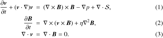$\begin{array}{ccc}\frac{\mathit{\partial }{v}}{\mathit{\partial t}}\mathrm{+}\mathrm{(}{v}\mathrm{·}\mathrm{\nabla }\mathrm{)}{v}& \mathrm{=}& \\ \frac{\mathit{\partial }{B}}{\mathit{\partial t}}& \mathrm{=}& \\ \mathrm{\nabla }\mathrm{·}{v}& \mathrm{=}& \end{array}$Here p is the plasma pressure and η the normalised resistivity. The viscous force is defined by the stress tensor whose form is discussed below. The MHD equations have been scaled using the typical coronal parameters: magnetic field strength B_c = 10²   G, length scale l_c = 10^9.5   cm, and number density n_c = 10⁹   cm^-3. Velocities are expressed in units of the Alfvén speed v_A = B_c/(4πρ_c)^1/2 ≃ 10⁹   cm  s^-1, where ρ_c = m_pn_c is the mass density and m_p is the proton mass.

Below we consider two alternative forms for the viscosity tensor: the classical isotropic viscosity 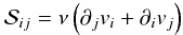${\mathrm{𝒮}}_{\mathit{ij}}\mathrm{=}\mathit{\nu }\mathrm{(}{\mathit{\partial }}_{\mathit{j}}{\mathit{v}}_{\mathit{i}}\mathrm{+}{\mathit{\partial }}_{\mathit{i}}{\mathit{v}}_{\mathit{j}}\mathrm{)}$(4)and the Braginskii (1965) form for the ion parallel viscosity 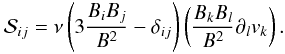${\mathrm{𝒮}}_{\mathit{ij}}\mathrm{=}\mathit{\nu }\left(\mathrm{3}\frac{{\mathit{B}}_{\mathit{i}}{\mathit{B}}_{\mathit{j}}}{{\mathit{B}}^{\mathrm{2}}}\mathrm{-}{\mathit{\delta }}_{\mathit{ij}}\right)\left(\frac{{\mathit{B}}_{\mathit{k}}{\mathit{B}}_{\mathit{l}}}{{\mathit{B}}^{\mathrm{2}}}{\mathit{\partial }}_{\mathit{l}}{\mathit{v}}_{\mathit{k}}\right)\mathit{.}$(5)As usual, summation over repeated indices is assumed. Although the form (4) is commonly employed, it becomes inaccurate in a magnetised plasma such as the solar corona. In such cases the Braginskii form that accounts for the anisotropies introduced by the magnetic field is more accurate (Hollweg 1986).

Two dimensionless parameters control the rate of energy dissipation, the resistivity η and the viscosity ν. Notably, although both are  ≪ 1, the coronal temperature interval (2 − 10) ×    10⁶ K implies that ν ≫ η, and so viscous dissipation is likely to dominate resistive dissipation in solar flares (e.g., Craig & Litvinenko 2009, and references therein). We use ${\mathit{W}}_{\mathrm{c}}\mathrm{=}{\mathit{v}}_{\mathrm{A}}{\mathit{l}}_{\mathrm{c}}^{\mathrm{2}}{\mathit{B}}_{\mathrm{c}}^{\mathrm{2}}\mathit{/}\mathrm{\left(}\mathrm{8}\mathit{\pi }\mathrm{\right)}\mathrm{\simeq }\mathrm{4}\mathrm{\times }{\mathrm{10}}^{\mathrm{30}}\hspace{0.17em}\mathrm{erg}{\mathrm{s}}^{-1}$ to scale the global energy dissipation rate. The dimensionless rate of resistive (Ohmic) dissipation is given by 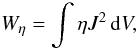${\mathit{W}}_{\mathit{\eta }}\mathrm{=}\mathrm{\int }\mathit{\eta }{\mathit{J}}^{\mathrm{2}}\hspace{0.17em}\mathrm{d}\mathit{V,}$(6)where J = ∇ × B is the current density. The viscous dissipation rate is given by ${\mathit{W}}_{\mathit{\nu }}\mathrm{=}\mathrm{\int }{\mathit{S}}_{\mathit{ij}}{\mathit{\partial }}_{\mathit{j}}{\mathit{v}}_{\mathit{i}}\hspace{0.17em}\hspace{0.17em}\mathrm{d}\mathit{V}\mathit{.}$(7)

2.2. Planar momentum and induction equations

Planar solutions for the magnetic and velocity fields can be expressed using flux and stream functions: ${B}\mathrm{=}\mathrm{\nabla }\mathit{\psi }\mathrm{\left(}\mathit{x,y,t}\mathrm{\right)}\mathrm{\times }{ẑ}\mathit{,} {v}\mathrm{=}\mathrm{\nabla }\mathit{\phi }\mathrm{\left(}\mathit{x,y,t}\mathrm{\right)}\mathrm{\times }{ẑ}\mathit{.}$(8)Since these forms satisfy Eq. (3) identically, the MHD equations reduce to $\begin{array}{ccc}\frac{\mathit{\partial }}{\mathit{\partial t}}\mathrm{(}{\mathrm{\nabla }}^{\mathrm{2}}{\mathit{\phi }}^{\mathrm{)}}\mathrm{+}\mathrm{\left[}{\mathrm{\nabla }}^{\mathrm{2}}\mathit{\phi ,}\hspace{0.17em}\mathit{\phi }\mathrm{\right]}& \mathrm{=}& \\ \frac{\mathit{\partial \psi }}{\mathit{\partial t}}\mathrm{+}\mathrm{\left[}\mathit{\psi ,}\hspace{0.17em}\mathit{\phi }\mathrm{\right]}& \mathrm{=}& \end{array}$where we use the Poisson bracket notation typified by

$\mathrm{[}\mathit{\psi ,}\hspace{0.17em}\mathit{\phi }\mathrm{]}\mathrm{=}{\mathit{\partial }}_{\mathit{x}}\mathit{\psi }\hspace{0.17em}{\mathit{\partial }}_{\mathit{y}}\mathit{\phi }\mathrm{-}{\mathit{\partial }}_{\mathit{y}}\mathit{\psi }\hspace{0.17em}{\mathit{\partial }}_{\mathit{x}}\mathit{\phi }\mathit{.}$Viscous effects are represented by $\mathit{G}\mathrm{=}\mathrm{-}\left(\mathrm{\nabla }\mathrm{\times }\mathrm{\nabla }\mathrm{·}\mathrm{𝒮}\right)\mathrm{·}{ẑ}\mathit{.}$(11)

3. Analytical models of magnetic merging

3.1. An exact visco-resistive model: classical viscosity

The simplest exact solution for magnetic merging is that of Sonnerup & Priest (1975). A stagnation point flow supports the steady annihilation of straight field lines advected towards a strong current layer centred on x = 0. Specifically the MHD equations are satisfied by 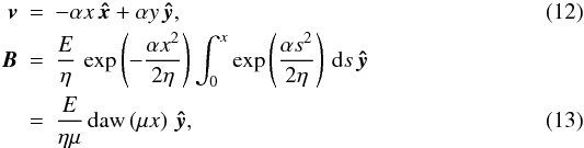$\begin{array}{ccc}{v}& \mathrm{=}& \\ {B}& \mathrm{=}& \frac{\mathit{E}}{\mathit{\eta }}\hspace{0.17em}\exp \left(\mathrm{-}\frac{\mathit{\alpha }{\mathit{x}}^{\mathrm{2}}}{\mathrm{2}\mathit{\eta }}\right){\mathrm{\int }}_{\mathrm{0}}^{\mathit{x}}\exp \left(\frac{\mathit{\alpha }{\mathit{s}}^{\mathrm{2}}}{\mathrm{2}\mathit{\eta }}\right)\hspace{0.17em}\mathrm{d}\mathit{s}\hspace{0.17em}{ŷ}\\ & \mathrm{=}& \end{array}$where the Dawson function is defined by

$\mathrm{daw}\mathrm{\left(}\mathit{s}\mathrm{\right)}\mathrm{=}{\mathrm{\int }}_{\mathrm{0}}^{\mathit{s}}\exp \mathrm{(}{\mathit{u}}^{\mathrm{2}}\mathrm{-}{\mathit{s}}^{\mathrm{2}}\mathrm{)}\hspace{0.17em}\mathrm{d}\mathit{u}$and μ² = α/2η. Here α determines the amplitude of the velocity field and E is a uniform electric field in the z-direction. The Dawson function identifies ${\mathit{x}}_{\mathit{s}}\mathrm{\simeq }\sqrt{\frac{\mathit{\eta }}{\mathit{\alpha }}}$(14)as the thickness of the current layer. This result implies the inflow and outflow speeds associated with the current sheet ${\mathit{v}}_{\mathrm{in}}\mathrm{\simeq }\sqrt{\mathit{\alpha \eta }}$ and v_out ≃ α. This solution can be generalised to include vortical and shear flows (Besser et al. 1990; Jardine et al. 1992). Another generalisation, valid only if ν = 0, is to allow the merging of curved field lines, leading to X-point reconnection (Craig & Henton 1995). None of these refinements significantly changes the scaling laws derived below.

Using Eqs. (4) and (7), the classical viscous dissipation rate in volume V is given by ${\mathit{W}}_{\mathit{\nu }}\mathrm{=}\mathrm{4}\mathit{\nu }{\mathit{\alpha }}^{\mathrm{2}}\hspace{0.17em}\mathit{V}\mathit{.}$(15)(In our numerical simulations, the volume is that of the cube 0 ≤ |x|,  |y|,  |z| ≤ 1.) The resistive dissipation is easy to estimate if the thinness of the sheet is exploited. Thus if B_s is the peak field strength in the current layer, then J ≃ B_s/x_s is the current density, and we have from Eq. (6) that ${\mathit{W}}_{\mathit{\eta }}\mathrm{\simeq }\mathrm{(}\mathit{\alpha \eta }{\mathrm{)}}^{\mathrm{1}\mathit{/}\mathrm{2}}{\mathit{B}}_{\mathit{s}}^{\mathrm{2}}\hspace{0.17em}\mathit{V}\mathit{.}$(16)Similarly, the rate of flux annihilation is $\mathit{E}\mathrm{=}\mathit{\eta J}\mathrm{\simeq }\mathrm{(}\mathit{\alpha \eta }{\mathrm{)}}^{\mathrm{1}\mathit{/}\mathrm{2}}{\mathit{B}}_{\mathit{s}}\mathit{.}$(17)The key aspect of these results is the presence of a single small scale x_s determined by the resistivity. Although viscous losses do occur, these arise from maintaining the global velocity field that drives the merging. By comparing Eqs. (15) and (16) and treating α and B_s as parameters of order unity, we see that viscous dissipation should dominate when ν > η^1/2. More physically, if we assume (as in Sweet-Parker merging) that exhaust speeds are related to the strength of the current layer, then it follows that α ≃ B_s (see Litvinenko & Craig 2000, for details), and so $\frac{{\mathit{W}}_{\mathit{\nu }}}{{\mathit{W}}_{\mathit{\eta }}}\mathrm{\simeq }\frac{\mathrm{4}}{{\mathit{B}}_{\mathit{s}}^{\mathrm{1}\mathit{/}\mathrm{2}}}\hspace{0.17em}\frac{\mathit{\nu }}{{\mathit{\eta }}^{\mathrm{1}\mathit{/}\mathrm{2}}}\mathrm{·}$(18)A similar result is obtained when the Braginskii viscosity is considered, as we now demonstrate.

3.2. An exact visco-resistive model: Braginskii viscosity

Exact solutions for magnetic merging, supported by vortical flows, have been obtained for the case of Braginskii viscosity. Both planar merging (Litvinenko 2005) and merging driven by three-dimensional flows (Craig & Litvinenko 2009) have been analysed.

We consider only the simplest planar solution, namely 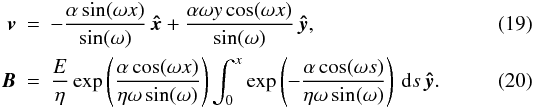$\begin{array}{ccc}{v}& \mathrm{=}& \mathrm{-}\frac{\mathit{\alpha }\sin \mathrm{\left(}\mathit{\omega x}\mathrm{\right)}}{\sin \mathrm{\left(}\mathit{\omega }\mathrm{\right)}}\hspace{0.17em}{x̂}\mathrm{+}\frac{\mathit{\alpha \omega y}\cos \mathrm{\left(}\mathit{\omega x}\mathrm{\right)}}{\sin \mathrm{\left(}\mathit{\omega }\mathrm{\right)}}\hspace{0.17em}{ŷ}\mathit{,}\\ {B}& \mathrm{=}& \end{array}$Here the parameter 0 ≤ ω < π determines the velocity gradient on the inflow boundary. Note that, as ω   → 0, the stagnation-point flow of the previous section is recovered. The parameters of the current layer (namely its thickness x_s and the inflow v_in and outflow v_out speeds) are all found to scale as those in the merging solution based on the classical viscosity.

The dimensionless dissipation rate, associated with the Braginskii viscosity, follows from Eqs. (5) and (7): ${\mathit{W}}_{\mathit{\nu }}\mathrm{=}\mathrm{3}\mathit{\nu }{\mathit{\alpha }}^{\mathrm{2}}\left(\frac{\mathrm{2}{\mathit{\omega }}^{\mathrm{2}}\mathrm{+}\mathit{\omega }\sin \mathrm{2}\mathit{\omega }}{\mathrm{4}{\sin }^{\mathrm{2}}\mathit{\omega }}\right)\hspace{0.17em}\mathit{V,}$(21)which reduces to 3να²   V as ω → 0. Since the reconnection rate and Ohmic dissipation rate are essentially unchanged from the previous model (at least provided ω does not approach π), we again recover Eq. (18) within factors of order unity.

3.3. The visco-resistive current layer

The previous two cases are based on exact solutions for large-scale velocity fields that drive the merging. By way of contrast, the following argument depends mainly on the local properties of the current layer. In particular, as in Park et al. (1983) and Craig & Litvinenko (2010), Sweet-Parker style arguments can be used to infer the emergence of a visco-resistive scale in the case ν ≫ η.

The argument is based on mass continuity, v_in = x_sv_out, steady flux transfer, v_inB_s = ηB_s/x_s, and pressure balance along and across the sheet. For a sufficiently large ν, the classical shear viscosity slows down the outflow and thickens up the current layer with the result that ${\mathit{x}}_{\mathit{s}}\mathrm{\simeq }\mathrm{(}\mathit{\eta \nu }{\mathrm{)}}^{\mathrm{1}\mathit{/}\mathrm{4}}{\mathit{B}}_{\mathit{s}}^{\mathrm{-}\mathrm{1}\mathit{/}\mathrm{2}}\mathit{.}$(22)The scaling for viscous dissipation is now based on the assumption that viscous damping is effective only within the narrow current layer–what happens outside the sheet is effectively neglected. The resulting dissipation scalings $\mathit{\eta J}\mathrm{\simeq }{\mathit{\eta }}^{\mathrm{3}\mathit{/}\mathrm{4}}{\mathit{\nu }}^{\mathrm{-}\mathrm{1}\mathit{/}\mathrm{4}}{\mathit{B}}_{\mathit{s}}^{\mathrm{3}\mathit{/}\mathrm{2}}\mathit{,}{\mathit{W}}_{\mathit{\eta }}\mathrm{\simeq }{\mathit{W}}_{\mathit{\nu }}\mathrm{\simeq }{\mathit{\eta }}^{\mathrm{3}\mathit{/}\mathrm{4}}{\mathit{\nu }}^{\mathrm{-}\mathrm{1}\mathit{/}\mathrm{4}}{\mathit{B}}_{\mathit{s}}^{\mathrm{5}\mathit{/}\mathrm{2}}\mathit{,}$(23)are quite different from the previous exact analytical models. These scalings (which correct a misprint in Eq. (20) of Craig & Litvinenko 2010) suggest that a large classical viscosity ν ≫ η should slow down the rate of magnetic merging. Note that when ν = η we obtain the traditional resistive Sweet-Parker scalings.

It is interesting that a similar analysis based on the Braginskii viscosity does not lead to the emergence of a visco-resistive scale, as pointed out by Craig & Litvinenko (2010). However, the scale x_s ~ (ην)^1/4 has also been obtained in an analytical model of slow magnetic reconnection at a two-dimensional X-point (Titov & Priest 1997), as well as in numerical studies of X-point collapse for both classical and Braginskii viscosities (Craig et al. 2005; Craig 2010).

To summarise, exact reconnection solutions exist for both classical and Braginskii viscosities, which do not contain a visco-resistive scale. By contrast, some analytical models and X-point simulations predict the emergence of the visco-resistive scale x_s ~ (ην)^1/4. Moreover, Sweet-Parker style scaling arguments imply that this scale should almost universally emerge in a viscous plasma with ν > η.

4. Visco-resistive simulations of magnetic reconnection

4.1. Numerical simulation

In this section we describe a series of side-by-side, flow-driven reconnection experiments using the Braginskii and classical viscosities. Typically the viscous coefficient ν is fixed at some representative value and scalings are derived by systematically reducing the resistivity η ≪ ν. To provide a further check on the results we also perform a “control” resistive simulation, based on the common numerical expedient of setting ν = η. That is, we would like to compare the visco-resistive reconnection scalings with those in the case ν = η, but, as is well known, setting ν = 0 is susceptible to numerical difficulties. Accordingly we set ν = η to approximate the purely resistive case (Biskamp 1994; Craig & Litvinenko 2010). Our aim is two-fold: first, to explore the emergence, or otherwise, of a visco-resistive scale; second, to quantify the differences that develop when classical and Braginskii viscosities are employed.

The results are obtained by numerically solving Eqs. (9) and (10), using a doubly periodic code over the region 0 ≤ |x|, |y| ≤ 1. Initial conditions are derived by assuming a vortical flow velocity field (clockwise in the first quadrant) given by $\mathit{\phi }\mathrm{\left(}\mathit{x,y,}\mathrm{0}\mathrm{\right)}\mathrm{=}\mathrm{-}\frac{{\mathit{\alpha }}_{\mathrm{0}}}{\mathit{\pi }}\sin \mathrm{\left(}\mathit{\pi x}\mathrm{\right)}\sin \mathrm{\left(}\mathit{\pi y}\mathrm{\right)}\mathit{,}$(24)where α₀ > 0 sets the amplitude of the initial flow. We assume an initial magnetic disturbance of the form 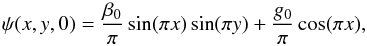$\mathit{\psi }\mathrm{\left(}\mathit{x,y,}\mathrm{0}\mathrm{\right)}\mathrm{=}\frac{{\mathit{\beta }}_{\mathrm{0}}}{\mathit{\pi }}\sin \mathrm{\left(}\mathit{\pi x}\mathrm{\right)}\sin \mathrm{\left(}\mathit{\pi y}\mathrm{\right)}\mathrm{+}\frac{{\mathit{g}}_{\mathrm{0}}}{\mathit{\pi }}\cos \mathrm{\left(}\mathit{\pi x}\mathrm{\right)}\mathit{,}$(25)where g₀ > 0 sets the amplitude of the magnetic disturbance and β₀ ≥ 0 controls the level of magnetic shear in the merging. In the simplest case of “head on” reconnection (β₀ = 0), initially straight field lines, washed together by the inflow, rapidly evolve, forming a well defined current layer centered on the origin.

To obtain resistive scalings, the parameters α₀, β₀ and ν are held fixed while η and g₀ are systematically reduced. Note that simply reducing η while keeping g₀ fixed would lead to high pressure, flux pile-up current sheets that would feed back on the flow and stall it. Accordingly, g₀ is adjusted to ensure that peak fields B_s in the reconnecting current layers have magnitudes of order unity. This allows us to obtain scalings at resistivities that are limited only by numerical resolution in the computation (the lowest values of resistivity considered here require mesh sizes  ≲ 10^-3). In practice we take α₀ = 1 and ν = 0.004 and allow resistivities in the range 10^-4.5 ≤ η ≤ 10^-2. Most of our simulations apply to head-on reconnection, β₀ = 0, but some preliminary results for sheared reconnection are given in Sect. 4.4.

As a final point we note that the Braginskii viscosity tensor (5) cannot be applied to fields that are very weak. Since our computation involves null points, it is convenient to adopt a form that effectively interpolates between the classical and Braginskii viscosities. In practice we adopt the “Liley” form of Hosking & Marinoff (1973).

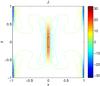Fig. 1 Contour plot of J taken at the time of maximum current density at the origin. The parameters are α0 = 1, β0 = 0 and η = ν = 0.004.

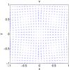Fig. 2 Arrow plot of v taken at the time of maximum current density at the origin. The parameters are the same as in Fig. 1, namely α0 = 1, β0 = 0 and η = ν = 0.004. For visual clarity only selected velocity vectors are displayed.

4.2. The reconnecting current sheet

Figures 1 and 2 show an example of a head-on Braginskii viscosity simulation with parameters α₀ = 1, β₀ = 0 and η = ν = 0.004. The dominant feature, which reaches maximum development after approximately one Alfvén time in the present simulation, is a strong current sheet centred on the origin. As discussed by Heerikhuisen et al. (2000), there is a good deal of numerical evidence to suggest that the properties of the current layer, when taken at the time of maximum current, can be accurately described by the steady merging models such as those discussed in Sect. 3.

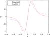Fig. 3 The y-component of the magnetic field in the current layer in the case of head-on merging. The parameters are the same as in Figs. 1 and 2. The solid line is the numerical magnetic field and the dashed line is the analytical solution from (13).

More specifically, suppose we use the fields displayed in Figs. 1 and 2 to evaluate the rate of flux transfer E and the inflow velocity amplitude α₀. The analytical solution (13) based on these parameters can then be compared with the simulated current layer. Figure 3 displays a slice of the simulated current sheet alongside the analytical model. Despite the fact that the analytic model is purely resistive and the vorticity parameter ω = 0, we see that the model provides a good representation of the dynamically evolved field in the current layer. The most obvious variations occur in the outer regions dominated by the large-scale vortical flows-the regions not accurately represented by the analytic, linear inflow model of (13). The implication is that Braginskii viscosity simulations are unlikely to undermine the form of the purely resistive current layer.

4.3. Head-on magnetic merging simulations

We now turn to quantifying the key parameters v_out, v_in, and x_s of the current layer and relating these to the global Ohmic and viscous energy release rates. Current sheet thickness is measured along the x axis at the level of half current maximum. Inflow and outflow velocities are measured on the x and y axes respectively at the current half maximum level. Figure 4 shows a comparison of the classical, Braginskii and ν = η control current sheet outflow speeds, calculated at the time of maximum current. Minor variations are apparent, and the outflow is generally slower in the case of the classical viscosity, yet the outflow speeds are essentially invariant with η. In particular, there is no evidence for a slowdown, v_out ~ (η/ν)^1/2, which would be caused by a visco-resistive scale in the case of classical viscosity (Sect. 3.3). The analytical scalings of Sect. 3.1 are clearly more accurate

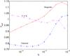Fig. 4 Current sheet outflow speed comparisons. Crosses, diamonds and circles refer to Braginskii, classical and ν = η control results respectively. The parameters are α0 = 1 and β0 = 0; ν = 0.004 for classical and Braginskii viscosity.

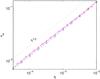Fig. 5 Current sheet inflow speed comparisons. Crosses, diamonds and circles refer to Braginskii, classical and ν = η control results respectively. The parameters are α0 = 1 and β0 = 0; ν = 0.004 for classical and Braginskii viscosity.

This interpretation is borne out by an analysis of the inflow speeds v_in and the current sheet thickness x_s, which both scale as η^1/2, as confirmed by the plots in Figs. 5 and 6. In both cases it is very difficult to distinguish the Braginskii, classical and ν = η control plots. The classical shear viscosity does provide the thickest current layer but the effect is marginal. This should be contrasted with the prediction x_s ~ (ην)^1/4 that follows from Sweet-Parker style arguments (Park et al. 1983).

The relation x_s ~ η^1/2 for the sheet thickness, coupled to the constraint B_s ≃ 1, leads to flux transfer and Ohmic dissipation rates that also follow the η^1/2 trend. These scalings are confirmed numerically for all three regimes (the ν = η control, the classical and Braginskii viscosities).

More interesting is the behaviour of the global viscous losses W_ν. As indicated in Fig. 7, the Braginskii and classical viscous losses are effectively invariant, but the ν = η control strongly decreases with η. The decline of the ν = η control, however, is slower than the expected W_ν ~ η scaling. We have confirmed that this behaviour is due to strong vortical flows associated with the very weak levels of viscous damping. When we weaken the magnetic field, washed in by the flow, the distortion diminishes and the expected scaling is regained. Nevertheless, this behaviour does indicate the enhanced sensitivity of the computation in the case of weak damping of the global velocity field.

Figure 8 plots the ratio of the viscous and resistive energy dissipation rates W_ν/W_η. As anticipated by Eq. (18) in the case of fixed ν, W_ν/W_η scales as η^1/2 as η is reduced. We see that, independent of the form of the viscosity, W_ν exceeds W_η by almost a factor of two at the lowest resistivity levels η ≤ 10^-4.

In summary, all the resistive scalings presented in this section appear consistent with the simple analytical models of Sects. 3.1 and 3.2. That is, for the flow-driven reconnection simulations considered here, the resistive scaling laws are effectively identical for both the Braginskii and classical viscosities. The limited role of the traditional scaling arguments (Park et al. 1983) should be emphasised. Although they provide a reliable description of the reconnecting current sheet in a nonviscous plasma, they do not give a valid description of magnetic reconnection in a viscous plasma, at least in the present, flow-driven simulations.

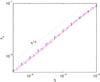Fig. 6 Current sheet thickness comparisons. The dotted line shows η1/2 scaling. Crosses, diamonds and circles refer to Braginskii, classical and ν = η control results respectively. The parameters are α0 = 1 and β0 = 0; ν = 0.004 for classical and Braginskii viscosity.

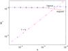Fig. 7 Viscous dissipation rate comparisons. Crosses, diamonds and circles refer to Braginskii, classical and ν = η control results respectively. The parameters are α0 = 1 and β0 = 0; ν = 0.004 for classical and Braginskii viscosity.

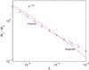Fig. 8 The ratio Wν/Wη for classical (diamonds) and Braginskii (crosses) viscosity. The dotted line shows η − 1/2 scaling. The parameters are α0 = 1, β0 = 0 and ν = 0.004.

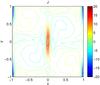Fig. 9 Current contour plot for sheared reconnection in the Braginskii case at time of maximum current density at the origin. The parameters are α0 = 1, β0 = 0.7, η = 0.004, and ν = 0.004.

4.4. Sheared magnetic reconnection simulations

As pointed out previously, it is possible to construct an analytical model for sheared magnetic reconnection only in the nonviscous case (Craig & Henton 1995). Guided by those exact resistive solutions, we expect that, compared with the head-on case, visco-resistive reconnection of sheared magnetic field lines should occur in thicker current sheets, which should lead to reduced energy dissipation and flux transfer rates. Figure 9 shows the current contour plot for a typical Braginskii run with a high value of shear (β₀ = 0.7). As in the head-on case, there is a well defined current sheet in the vicinity of the magnetic null, but there is now significant warping of the ends of the sheet.

Our numerical results show that, even with relatively high levels of shearing, the classical viscosity results essentially follow the same scalings as in the head-on case (x_s ~ η^1/2,  W_η ~ η^1/2,  W_ν ~ η⁰). Systematic deviations, however, appear in the case of the Braginskii viscosity for high levels of shearing. These deviations from the analytical predictions imply that the structure of the current sheet is significantly modified by the anisotropic Braginskii viscous forces when the reconnecting magnetic field lines are strongly sheared. Unfortunately, as yet, visco-resistive analytical solutions are only available for head-on reconnection.

Figure 10 illustrates the main new effect of strong magnetic shear (cf. Fig. 8). It shows W_ν/W_η for the classical and Braginskii viscosities in the case β₀ = 0.7. For the classical viscosity, both the resistive dissipation rate W_η and the viscous dissipation rate W_ν agree with the analytical arguments, leading to Eq. (18). The ratio W_ν/W_η for the Braginskii viscosity, however, appears to follow a different scaling (closer to η^-1). We confirmed that this deviation is due to a slow down in the resistive dissipation rate (this scales closer to η rather than η^1/2) in the strongly sheared Braginskii simulation.

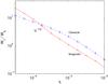Fig. 10 The ratio Wν/Wη for classical (diamonds) and Braginskii (crosses) viscosity. The dotted line shows η − 1/2 scaling. The parameters are α0 = 1, β0 = 0.7 and ν = 0.004.

5. Conclusions

Given the smallness of the electric resistivity in most astrophysical application, the search for a robust fast mechanism of magnetic reconnection has provided the motivation for a great deal of work on reconnection theory. Both analytical and numerical studies suggest that viscous dissipation may be capable of dominating resistive dissipation under a wide variety of coronal conditions (Hollweg 1986; Litvinenko 2005; Craig & Litvinenko 2009). However, as we discussed in Sect. 3, analytical studies of magnetic reconnection in a resistive viscous plasma lead to contradictory results. Some analytical solutions predict the formation of a current layer on the visco-resistive scale  ~(ην)^1/4, while other solutions do not contain this scale. This key difference leads to different predictions for the parameters of the reconnecting current sheet and the dependence of the energy release rate on the viscous and resistive coefficients.

In this paper, we attempted to clarify the issue by performing numerical simulations of planar magnetic reconnection in periodic geometry. We considered head-on reconnection, driven by large-scale vortical flows in an incompressible plasma. We used both the classical shear viscosity and the Braginskii form for the ion parallel viscosity in a magnetised plasma. Somewhat surprisingly, our numerical results show that the parameters of the reconnecting current sheet (its thickness, the inflow and outflow speeds) are accurately described by purely resistive analytical scalings of flux pile-up magnetic merging, regardless of the form of the viscous stress tensor. The computed global resistive and viscous energy dissipation rates also closely follow Eq. (18), confirming that the current sheet thickness is effectively independent of viscosity for both the classical and Braginskii forms.

We have also made a preliminary study of the properties of the reconnection region in the case of a strong magnetic shear. It appears that in the Braginskii case magnetic shearing can modify the dissipation scalings, implying that the properties of the reconnecting current sheet depend on the form of the viscosity. This potentially important result requires further investigation. Interpreting numerical results in strongly sheared reconnection is not straightforward, since the available visco-resistive analytical solutions are only able to describe head-on merging.

To summarise, we find no evidence of the visco-resistive scale  ~(ην)^1/4 and the corresponding energy release rate scalings in our simulations of planar magnetic reconnection in periodic geometry. This finding contrasts sharply with predictions of some steady analytical models, Sweet-Parker style scaling arguments, and time-dependent simulations in a closed X-point geometry. There appears to be no simple criterion for the emergence of the visco-resistive scale.

Our results may be partly due to there not being enough time for the visco-resistive scale to develop: we took the current sheet parameters at the time of the first current maximum (first implosion), and it may be that the scale would develop after several implosions. Either way, the precise conditions required to ensure the emergence of a visco-resistive scale remain unclear. We believe that further analytic and numerical work is warranted, given the potential importance of viscous dissipation

arising from either classical or Braginskii viscosity in solar flares and other astrophysical applications.

Acknowledgments

This work was supported by NSF grant ATM-0734032 and NASA grant NNX08AG44G.

References

All Figures

	Fig. 1 Contour plot of J taken at the time of maximum current density at the origin. The parameters are α0 = 1, β0 = 0 and η = ν = 0.004.
In the text

	Fig. 2 Arrow plot of v taken at the time of maximum current density at the origin. The parameters are the same as in Fig. 1, namely α0 = 1, β0 = 0 and η = ν = 0.004. For visual clarity only selected velocity vectors are displayed.
In the text

	Fig. 3 The y-component of the magnetic field in the current layer in the case of head-on merging. The parameters are the same as in Figs. 1 and 2. The solid line is the numerical magnetic field and the dashed line is the analytical solution from (13).
In the text

	Fig. 4 Current sheet outflow speed comparisons. Crosses, diamonds and circles refer to Braginskii, classical and ν = η control results respectively. The parameters are α0 = 1 and β0 = 0; ν = 0.004 for classical and Braginskii viscosity.
In the text

	Fig. 5 Current sheet inflow speed comparisons. Crosses, diamonds and circles refer to Braginskii, classical and ν = η control results respectively. The parameters are α0 = 1 and β0 = 0; ν = 0.004 for classical and Braginskii viscosity.
In the text

	Fig. 6 Current sheet thickness comparisons. The dotted line shows η1/2 scaling. Crosses, diamonds and circles refer to Braginskii, classical and ν = η control results respectively. The parameters are α0 = 1 and β0 = 0; ν = 0.004 for classical and Braginskii viscosity.
In the text

	Fig. 7 Viscous dissipation rate comparisons. Crosses, diamonds and circles refer to Braginskii, classical and ν = η control results respectively. The parameters are α0 = 1 and β0 = 0; ν = 0.004 for classical and Braginskii viscosity.
In the text

	Fig. 8 The ratio Wν/Wη for classical (diamonds) and Braginskii (crosses) viscosity. The dotted line shows η − 1/2 scaling. The parameters are α0 = 1, β0 = 0 and ν = 0.004.
In the text

	Fig. 9 Current contour plot for sheared reconnection in the Braginskii case at time of maximum current density at the origin. The parameters are α0 = 1, β0 = 0.7, η = 0.004, and ν = 0.004.
In the text

	Fig. 10 The ratio Wν/Wη for classical (diamonds) and Braginskii (crosses) viscosity. The dotted line shows η − 1/2 scaling. The parameters are α0 = 1, β0 = 0.7 and ν = 0.004.
In the text

References

- Besser, B. P., Biernat, H. K., & Rijnbeek, R.P. 1990, Planet. Space Sci., 38, 411 [NASA ADS] [CrossRef] [Google Scholar]
- Biskamp, D. 1994, Phys. Rep., 237, 179 [NASA ADS] [CrossRef] [Google Scholar]
- Braginskii, S. I. 1965, Rev. Plasma Phys., 1, 205 [NASA ADS] [Google Scholar]
- Craig, I. J. D. 2010, A&A, 515, A96 [NASA ADS] [CrossRef] [EDP Sciences] [Google Scholar]
- Craig, I. J. D., & Henton, S. M. 1995, ApJ, 450, 280 [NASA ADS] [CrossRef] [Google Scholar]
- Craig, I. J. D., & Litvinenko, Y. E. 2009, A&A, 501, 755 [NASA ADS] [CrossRef] [EDP Sciences] [Google Scholar]
- Craig, I. J. D., & Litvinenko, Y. E. 2010, ApJ, 725, 886 [NASA ADS] [CrossRef] [Google Scholar]
- Craig, I. J. D., Litvinenko, Y. E., & Senanayake, T. 2005, A&A, 433, 1139 [NASA ADS] [CrossRef] [EDP Sciences] [Google Scholar]
- Heerikhuisen, J., Craig, I. J. D., & Watson, P. G. 2000, Geophys. Astrophys. Fluid Dyn., 93, 115 [NASA ADS] [CrossRef] [Google Scholar]
- Hollweg, J. V. 1985, J. Geophys. Res., 90, 7620 [NASA ADS] [CrossRef] [Google Scholar]
- Hollweg, J. V. 1986, ApJ, 306, 730 [NASA ADS] [CrossRef] [Google Scholar]
- Hosking, R. J., & Marinoff, G. M. 1973, Plasma Phys., 15, 327 [NASA ADS] [CrossRef] [Google Scholar]
- Jardine, M., Allen, H. R., Grundy, R. E., & Priest, E. R. 1992, J. Geophys. Res., 97, 4199 [NASA ADS] [CrossRef] [Google Scholar]
- Litvinenko, Y. E. 2005, Sol. Phys., 229, 203 [NASA ADS] [CrossRef] [Google Scholar]
- Litvinenko, Y. E., & Craig, I. J. D. 2000, ApJ, 544, 1101 [NASA ADS] [CrossRef] [Google Scholar]
- Litvinenko, Y. E., & Craig, I. J. D. 2003, Sol. Phys., 218, 173 [NASA ADS] [CrossRef] [Google Scholar]
- Montgomery, D. 1992, J. Geophys. Res., 97, 4309 [NASA ADS] [CrossRef] [Google Scholar]
- Park, W., Monticello, D. A., & White, R. B. 1983, Phys. Fluids, 27, 137 [Google Scholar]
- Parker, E. N. 1957, J. Geophys. Res., 62, 509 [Google Scholar]
- Priest, E. R., & Forbes, T. 2000, Magnetic reconnection: MHD theory and applications (Cambridge Univ. Press) [Google Scholar]
- Rüdiger, G., & Kitchatinov, L. L. 1997, Astron. Nach., 318, 273 [CrossRef] [Google Scholar]
- Sonnerup, B. U. Ö., & Priest, E. R. 1975, Plasma Phys., 14, 283 [Google Scholar]
- Titov, V. S., & Priest, E. R. 1997, J. Fluid Mech., 348, 327 [NASA ADS] [CrossRef] [Google Scholar]