| Issue |
A&A
Volume 533, September 2011
|
|
|---|---|---|
| Article Number | A108 | |
| Number of page(s) | 5 | |
| Section | Astrophysical processes | |
| DOI | https://doi.org/10.1051/0004-6361/201116642 | |
| Published online | 09 September 2011 | |
Global dynamo models from direct numerical simulations and their mean-field counterparts
MAG (ENS/IPGP), LRA, Ecole Normale Supérieure, 24 rue Lhomond,
75252
Paris Cedex 05,
France
e-mail: This email address is being protected from spambots. You need JavaScript enabled to view it.
Received:
3
February
2011
Accepted:
24
June
2011
Abstract
Context. The test-field method permits us to compute dynamo coefficients from global, direct numerical simulations. The subsequent use of these parameters in mean-field models enables us to compare self-consistent dynamo models with their mean-field counterparts. This has been done to date for a simulation of rotating magnetoconvection and a simple benchmark dynamo, which are both (quasi-)stationary.
Aims. It is shown that chaotically time-dependent dynamos in a low Rossby number regime can be appropriately described by corresponding mean-field results. We also identify conditions under which mean-field models disagree with direct numerical simulations.
Methods. We solve the equations of magnetohydrodynamics (MHD) in a rotating, spherical shell in the Boussinesq approximation. Based on this, we compute mean-field coefficients for several models with the help of the previously developed test-field method. The parameterization of the mean electromotive force by these coefficients is tested against direct numerical simulations. In addition, we use the determined dynamo coefficients in mean-field models and compare the outcome with azimuthally averaged fields from direct numerical simulations.
Results. The azimuthally and time-averaged electromotive force in rapidly rotating dynamos is sufficiently well parameterized by the set of determined mean-field coefficients. In comparison to the previously considered (quasi-)stationary dynamo, the chaotic time-dependence leads to an improved scale separation and thus to a closer agreement between direct numerical simulations and mean-field results.
Key words: methods: numerical / magnetohydrodynamics (MHD) / dynamo
© ESO, 2011
1. Introduction
Mean-field electrodynamics provides a conceptual understanding of dynamo processes
generating coherent, large-scale magnetic fields in planets, stars, and galaxies (Krause & Rädler 1980; Moffatt 1978). However, it depends on a number of free parameters, that
are only poorly known under astrophysically relevant conditions. We briefly summarize the
essentials of mean-field theory to specify this point. Within a mean-field approach, the
velocity and the magnetic field are usually divided into large-scale mean fields,
 , and
residual parts,
v,b, that
vary on much shorter length or timescales,
, and
residual parts,
v,b, that
vary on much shorter length or timescales,  (1)The evolution of the
mean field is then governed by
(1)The evolution of the
mean field is then governed by  (2)In the above equation,
the mean electromotive force is defined as
(2)In the above equation,
the mean electromotive force is defined as  and η is the magnetic diffusivity. Equation (2) is coupled with an equation for the residual
field
and η is the magnetic diffusivity. Equation (2) is coupled with an equation for the residual
field  (3)in which
G is defined as
G = v ×
(3)in which
G is defined as
G = v ×
 .
The above system of equations is equivalent to the usual induction equation and no
approximation has been applied so far. An important simplification of the mean-field
approach consists of considering Eq. (2)
alone, which requires us to express ℰ as a linear functional
of
.
The above system of equations is equivalent to the usual induction equation and no
approximation has been applied so far. An important simplification of the mean-field
approach consists of considering Eq. (2)
alone, which requires us to express ℰ as a linear functional
of  ,
and
,
and  .
This is justified by Eq. (3), and we
may write
.
This is justified by Eq. (3), and we
may write 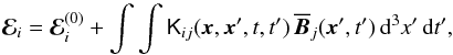 (4)in which K denotes
some integral kernel and we refer for the moment to cartesian coordinates. The
term ℰ(0) in Eq. (4) accounts for small-scale dynamo action and is not considered here but
discussed later. In addition, we assume that ℰ depends only
instantaneously and nearly locally on .
This is crucial and is referred to as the assumption of scale separation in the following.
Therefore,
in Eq. (4) may be replaced by its rapidly
converging Taylor series expansion at x,
(4)in which K denotes
some integral kernel and we refer for the moment to cartesian coordinates. The
term ℰ(0) in Eq. (4) accounts for small-scale dynamo action and is not considered here but
discussed later. In addition, we assume that ℰ depends only
instantaneously and nearly locally on .
This is crucial and is referred to as the assumption of scale separation in the following.
Therefore,
in Eq. (4) may be replaced by its rapidly
converging Taylor series expansion at x, 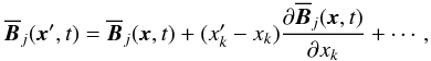 (5)and taken out of the
integral
(5)and taken out of the
integral  (6)where
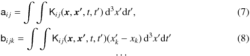 The
dynamo coefficients a and b defined in Eqs. (7) and (7) together with the
expansion in Eq. (6) may finally be used to
solve Eq. (2). Moreover, a and b are directly
linked to dynamo processes, i.e. to the generation, advection, and diffusion of the mean
magnetic field, thus provide physical concepts to explain dynamo action (e.g. Rädler 1995). Unfortunately, they are not known in
general and previous work often relies on arbitrary assumptions about them.
The
dynamo coefficients a and b defined in Eqs. (7) and (7) together with the
expansion in Eq. (6) may finally be used to
solve Eq. (2). Moreover, a and b are directly
linked to dynamo processes, i.e. to the generation, advection, and diffusion of the mean
magnetic field, thus provide physical concepts to explain dynamo action (e.g. Rädler 1995). Unfortunately, they are not known in
general and previous work often relies on arbitrary assumptions about them.
The test-field method by Schrinner et al. (2005, 2007) permits us to compute a and b from direct numerical simulations. It was first applied to a simulation of rotating magnetoconvection (Olson et al. 1999) and a simple geodynamo simulation (Christensen et al. 2001), which are both stationary except for an azimuthal drift. In the past three years, the test-field method was intensively used to compute mean-field coefficients for box simulations (e.g. Sur et al. 2008; Gressel et al. 2008; Brandenburg 2009; Käpylä et al. 2009; Rädler & Brandenburg 2009), which are not the focus of this paper. Although the test-field method proved to be reliable, the parameterization of the electromotive force for the steady geodynamo model was unsatisfactory. The expansion in Eq. (6) does not converge for this steady example because of a non-sufficient scale separation (Schrinner et al. 2007). In this paper, we revisit the problem for chaotically time-dependent dynamos. We test azimuthally and time-averaged electromotive-force vectors against their parameterization based on corresponding dynamo coefficients and compare azimuthally and time-averaged fields from direct numerical simulations with mean-field results.
2. Dynamo simulations
We solve the equations of magnetohydrodynamics (MHD) in the Boussinesq approximation for a
conducting fluid in a rotating spherical shell as given by Olson et al. (1999),  The
coupled differential equations for the the velocity V, the
magnetic field B, and the temperature T are
governed by four parameters. These are the Ekman number
E = ν/ΩL2,
the (modified) Rayleigh number
Ra = αTg0ΔTL/νΩ,
the Prandtl number
Pr = ν/κ, and the
magnetic Prandtl number
Pm = ν/η. In these
expressions, ν denotes the kinematic viscosity, Ω the rotation rate,
L the shell width, αT the thermal expansion
coefficient, g0 is the gravitational acceleration at the outer
boundary, ΔT stands for the temperature difference between the spherical
boundaries, κ is the thermal and
η = 1/μσ the magnetic diffusivity
with the magnetic permeability μ, and the electrical
conductivity σ. In addition to these input parameters, we introduce the
magnetic Reynolds number
Rm = Vrms L/η,
and the local Rossby number
The
coupled differential equations for the the velocity V, the
magnetic field B, and the temperature T are
governed by four parameters. These are the Ekman number
E = ν/ΩL2,
the (modified) Rayleigh number
Ra = αTg0ΔTL/νΩ,
the Prandtl number
Pr = ν/κ, and the
magnetic Prandtl number
Pm = ν/η. In these
expressions, ν denotes the kinematic viscosity, Ω the rotation rate,
L the shell width, αT the thermal expansion
coefficient, g0 is the gravitational acceleration at the outer
boundary, ΔT stands for the temperature difference between the spherical
boundaries, κ is the thermal and
η = 1/μσ the magnetic diffusivity
with the magnetic permeability μ, and the electrical
conductivity σ. In addition to these input parameters, we introduce the
magnetic Reynolds number
Rm = Vrms L/η,
and the local Rossby number  as
important output parameters. For the latter parameter definitions,
Vrms denotes the rms-velocity
and
as
important output parameters. For the latter parameter definitions,
Vrms denotes the rms-velocity
and  is the mean
half-wavelength of the flow derived from the kinetic energy spectrum (Christensen & Aubert 2006).
is the mean
half-wavelength of the flow derived from the kinetic energy spectrum (Christensen & Aubert 2006).
No-slip mechanical boundary conditions were chosen for all simulations presented here and the magnetic field continues as a potential field outside the fluid shell. Convection is driven by an imposed temperature difference between the inner and the outer shell shell-boundary.
3. Computation of dynamo coefficients
To determine the dynamo coefficients a and b, we apply the test-field method explained in
full detail in Schrinner et al. (2007). The principal
idea of this approach is to measure the mean electromotive force generated by the
interaction of the flow with an arbitrarily imposed test
field,  . The imposed test field
appears as an inhomogeneity in Eq. (3),
. The imposed test field
appears as an inhomogeneity in Eq. (3),
 (12)which is solved
simultaneously with Eqs. (9)−(11). The electromotive force due to a
given
(12)which is solved
simultaneously with Eqs. (9)−(11). The electromotive force due to a
given  may then be computed as
 with b resulting from Eq. (12). Finally, ℰT is used to solve
Eq. (6) for the dynamo coefficients.
To close the resulting system of linear equations and determine all components of a and b,
the numerical experiment in Eq. (12) must be
repeated several times with different fields .
with b resulting from Eq. (12). Finally, ℰT is used to solve
Eq. (6) for the dynamo coefficients.
To close the resulting system of linear equations and determine all components of a and b,
the numerical experiment in Eq. (12) must be
repeated several times with different fields .
So far, averaged quantities labelled by an overbar are axisymmetric fields,
whereas v and b in (12) are non-axisymmetric residuals. For a
stochastically stationary but nevertheless chaotically time-dependent flow,
ℰ and the mean-field coefficients vary in time. Thus, we introduce an
additional time-averaging indicated by brackets, ⟨ ··· ⟩ , and write  (13)instead of
Eq. (6). In the above equation,
ℰ has been time-averaged,
(13)instead of
Eq. (6). In the above equation,
ℰ has been time-averaged,  (14)and a and b also denote
time-averaged tensors. Furthermore, we interpret averages in Eq. (2) as combined azimuthal and time averages.
Neither is formally correct. However, the approximations applied can be justified, if
(14)and a and b also denote
time-averaged tensors. Furthermore, we interpret averages in Eq. (2) as combined azimuthal and time averages.
Neither is formally correct. However, the approximations applied can be justified, if
-
i)
temporal fluctuations of the axisymmetric velocity andmagnetic field are comparatively small, and
-
ii)
time averages of the non-axisymmetric residuals of the velocity and the magnetic field are negligible.
4. Comparison of mean-field results with direct numerical simulations
Mean-field coefficients determined from direct numerical simulations may be used in
mean-field models. Subsequently, azimuthally and time-averaged magnetic fields resulting
from three-dimensional, self-consistent models may be compared with their mean-field
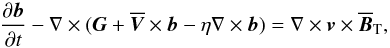
counterparts. Mean-field calculations presented here are based on Eq. (2) written as an eigenvalue problem  (15)in which the linear
operator D is defined as
(15)in which the linear
operator D is defined as  (16)and a and b are
time-averaged dynamo coefficients as described above. The eigenvalues σ
lead to a time evolution of each mode that is proportional to exp(σt). For
more details about the eigenvalue calculation, we refer to Schrinner et al. (2010b).
(16)and a and b are
time-averaged dynamo coefficients as described above. The eigenvalues σ
lead to a time evolution of each mode that is proportional to exp(σt). For
more details about the eigenvalue calculation, we refer to Schrinner et al. (2010b).
In addition, the parameterization of the electromotive force by dynamo coefficients,
i.e. Eq. (6), may be tested against the
mean electromotive force in direct numerical simulations. Again by virtue of Eqs. (13), (14), we compare ℰ as given in Eq. (14) and derived directly from numerical
models, with  (17)in which
 and
and
 are also obtained from direct
numerical simulations. Furthermore, we follow Schrinner
et al. (2007) and introduce
are also obtained from direct
numerical simulations. Furthermore, we follow Schrinner
et al. (2007) and introduce
 (18)in
order to quantify errors in the parameterization of ℰ.
(18)in
order to quantify errors in the parameterization of ℰ.
5. Results
Overview of the models considered, ordered with respect to their local Rossby number.
Besides the (quasi-)steady benchmark dynamo (model 1), we considered six chaotically time-dependent dynamos. The models are defined by four control parameters; E, Ra, and Pm were varied (see Table 1), whereas the Prandtl number was kept fixed and set to 1 for all simulations. The local Rossby number is always lower than 0.12 for the models considered here. They therefore belong to the regime of kinematically stable dynamos (Schrinner et al. 2010a). To simplify the time averaging, models with low and fairly moderate Rm were chosen. The resulting velocity fields are almost symmetric with respect to the equatorial plane, except for model 7, and convection occurs mainly outside the inner core tangent cylinder. Figure 1 shows the volume-averaged kinetic energy density for model 3 and illustrates the irregular time-dependence of these models.
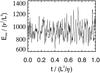 |
Fig. 1 Volume-averaged kinetic energy density versus magnetic diffusion time for model 3. |
The parameterization of the mean electromotive force given by Eq. (17) was found to be more suitable for the chaotically time-dependent dynamos than the benchmark dynamo; Δℰ decreases by more than a factor of 4 from model 1 to model 7. The considerable decline in Δℰ from the steady to the time-dependent models is most clearly visible in Fig. 2. It shows Δℰ for different models versus their magnetic Reynolds number. Apart from the aforementioned difference between the time-dependent and the stationary models, a dependence of Δℰ on Rm cannot be inferred.
In addition, the growth rate of the leading eigenmode of D, λ = ℜ(σ), may be taken as a measure for the accuracy of the mean-field description. Ideally, it is 0, whereas all overtones are highly diffusive (Schrinner et al. 2010a, 2011b). For numerical simulations, however, it is impossible to hit the critical point exactly. The growth rates of the fundamental mode for all models are given in Table 1 in units of η/L2. We note that the turbulent diffusivity largely exceeds the molecular one. For model 2, for instance, we find values of β-components up to 63η. Thus, for model 2, 1/λ ≈ 1/7 L2/η is much larger than one effective decay time and the fundamental mode is already near its critical state. With decreasing Δℰ, the growth rates become even smaller and the values closest to zero have been obtained for models 5−7.
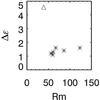 |
Fig. 2 Δℰ versus the magnetic Reynolds number for the (quasi)-stationary benchmark dynamo (triangle) and the six chaotically time-dependent dynamos considered. |
Model 7 provided the closest fitting and enabled Δℰ = 1.1 to be achieved. This is still clearly larger than for the simulation of rotating magnetoconvection for which Δℰ = 0.28 was found by Schrinner et al. (2007). Figure 3 compares ℰ to ℰ(1). Differences are visible in all components, but also principal similarities.
Figure 4 compares the azimuthally and time-averaged magnetic field resulting from direct numerical simulations with the fundamental eigenmode of D for model 7. Apart from small differences, direct numerical simulations and mean-field calculations agree very well for this example.
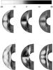 |
Fig. 3 Contour plots of ℰr, ℰθ, and
ℰφ (top line, from left to right) and
|


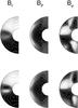 |
Fig. 4 Comparison between direct numerical simulations and mean-field calculations for model 7. Bottom line: azimuthally and time-averaged magnetic field obtained by solving (9)−(11). Top line: fundamental eigenmode resulting from (15). Each component has been normalised with respect to its absolute maximum. Therefore, the greyscale coding varies from −1, white, to + 1, black, and the contour lines correspond to ±0.1, ±0.3, ±0.5 ±0.7, ±0.9. |
6. Discussion
We do not derive mean-field coefficients for time-averaged mean fields in a formal sense.
The comparisons in Figs. 3 and 4 are motivated by assumptions i) and ii) in Sect. 3, instead. They are reasonably well fulfilled for the simulations
considered here. For model 7, v time-averaged over 30 magnetic
diffusion times declines sharply to 0.1% of V. A similar
decrease has been found for b. Moreover, the axisymmetric flow
and the axisymmetric magnetic field show comparatively little time variation. The
time-dependent components of  and
are of the order of 8% (37%) and 17% (23%) of the total (axisymmetric) flow and the total
(axisymmetric) magnetic field, respectively. In other words, time-averaging results in
axisymmetric fields and azimuthal averaging somewhat reduces the time variability. Combining
both leads to an extended averaging and thus to an improved scale separation. This finding
is also supported by Figs. 5 and 6. Figure 5 shows a noticeable
decrease of Δℰ for model 5, if the time-averaging period τ is increased.
Δℰ drops rapidly until
τ ≈ 2L2/η;
an extension of the time-averaging interval over more than 2 magnetic diffusion times
improves the scale separation only slightly. Moreover, Fig. 6 compares the residual with the mean magnetic field for model 1 (upper panel) and
model 7 (lower panel). In contrast to model 1, the time-dependent residual and the
time-averaged mean magnetic field of model 7 vary on fairly different length-scales. Thus,
a clearer scale separation for the time-dependent models seems to be plausible.
Consequently, Δℰ drops drastically from model 1 to model 2. However, there are still
noticeable differences between ℰ
and ℰ(1) in Fig. 3 for model 7. On the basis of this comparison alone,
it would be difficult to decide, whether the parameterization of ℰ
is already satisfactory. Additional support for its reliability comes from the good
agreement between the results of direct numerical simulations and mean-field modeling in
Fig. 4. Contour plots of all three components of the
leading eigenmode of D agree well with corresponding results from direct numerical
simulations. Moreover, the growth rates of the leading eigenmodes are close to zero,
as expected for stochastically stationary dynamos in the kinematically stable regime.
and
are of the order of 8% (37%) and 17% (23%) of the total (axisymmetric) flow and the total
(axisymmetric) magnetic field, respectively. In other words, time-averaging results in
axisymmetric fields and azimuthal averaging somewhat reduces the time variability. Combining
both leads to an extended averaging and thus to an improved scale separation. This finding
is also supported by Figs. 5 and 6. Figure 5 shows a noticeable
decrease of Δℰ for model 5, if the time-averaging period τ is increased.
Δℰ drops rapidly until
τ ≈ 2L2/η;
an extension of the time-averaging interval over more than 2 magnetic diffusion times
improves the scale separation only slightly. Moreover, Fig. 6 compares the residual with the mean magnetic field for model 1 (upper panel) and
model 7 (lower panel). In contrast to model 1, the time-dependent residual and the
time-averaged mean magnetic field of model 7 vary on fairly different length-scales. Thus,
a clearer scale separation for the time-dependent models seems to be plausible.
Consequently, Δℰ drops drastically from model 1 to model 2. However, there are still
noticeable differences between ℰ
and ℰ(1) in Fig. 3 for model 7. On the basis of this comparison alone,
it would be difficult to decide, whether the parameterization of ℰ
is already satisfactory. Additional support for its reliability comes from the good
agreement between the results of direct numerical simulations and mean-field modeling in
Fig. 4. Contour plots of all three components of the
leading eigenmode of D agree well with corresponding results from direct numerical
simulations. Moreover, the growth rates of the leading eigenmodes are close to zero,
as expected for stochastically stationary dynamos in the kinematically stable regime.
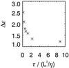 |
Fig. 5 Δℰ for model 5 varying with increasing time-averaging period τ. |
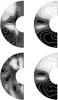 |
Fig. 6 Upper panel: non-axisymmetric radial magnetic field at arbitrary longitude (left) and azimuthally-averaged radial magnetic field (right) for model 1. Lower panel: non-axisymmetric and time-dependent radial magnetic field at arbitrary longitude and time (left) and azimuthally and time-averaged radial magnetic field (right) for model 7. The style of the contour plots is the same as in Fig. 4. |
Dynamo action in stars and planetary cores most probably takes place on a wide range of length and time scales. Owing to computational limitations, numerical simulations do not cover the whole range of scales possibly involved. Global dynamo simulations focus only on large scales, and we typically do not find small-scale dynamo action as reported for box simulations (e.g. Vögler & Schüssler 2007). Therefore, the component of the electromotive force independent of the mean magnetic field, i.e. ℰ(0) in (4), is zero for most global dynamo simulations. The possibility of a contribution to ℰ from small-scale dynamo action has been intensively discussed in the literature (e.g. Rädler 1976; Rädler 2000; Rädler & Rheinhardt 2007). It has been used to argue against the applicability of mean-field theory (Cattaneo & Hughes 2009). However, the conceptual difficulties that might result from simultaneous small- and large-scale dynamo action are at present irrelevant to the approach followed here.
The problem of scale separation has been addressed in this study only on spatial scales. This seems to be appropriate because we intend to describe stochastically stationary mean-fields with zero growth rate resulting from self-consistent dynamo simulations. More generally, time derivatives of the mean field in the expansion of ℰ have to be taken into account. As for non-local effects (Brandenburg et al. 2008), memory effects of the flow may also influence the parameterization of the electromotive force (Hubbard & Brandenburg 2009; Hughes & Proctor 2010).
Mean-field theory as presented here is intrinsically a kinematic approach. In general, an eigenvalue calculation based on Eq. (15) will lead to growing modes, even if the mean-field coefficients are derived from a saturated velocity field (Tilgner & Brandenburg 2008; Cattaneo & Tobias 2009). In this situation, mean-field models might not agree with direct numerical simulations, unless a more self-consistent extension of the theoretical framework and the test-field method is applied (Courvoisier et al. 2010; Rheinhardt & Brandenburg 2010). However, the class of chaotically time-dependent dynamos we considered is kinematically stable. Schrinner et al. (2010a) identified a regime of rapidly rotating dynamos that are dominated by only one dipolar mode at marginal stability, whereas all overtones are highly diffusive. A saturated velocity field from this class of dynamos does not lead to exponential growth of the magnetic field in a corresponding kinematic calculation. Consequently, the mean-field approach based on Eq. (15) is applicable to this dynamo regime, as confirmed once more in this study. In particular for models beyond this regime, the reliability of the mean-field approach presented here is not guaranteed and has to be demonstrated to be plausible by a comparison with direct numerical simulations (e.g. Schrinner et al. 2011a).
7. Summary
The mean-field description of a (quasi-)stationary dynamo has been affected by a poor scale-separation, hence from an insufficiently accurate parameterization of the electromotive force (Schrinner et al. 2007). We have demonstrated that the chaotically time-dependent dynamos considered here can provide improvements in both cases, if a combined azimuthal and time average is applied. The more accurate parameterization of ℰ leads to close agreement between mean-field models and direct numerical simulations: field topologies and growth rates resulting from both approaches have indeed be shown to be very similar.
In conclusion, the test-field method for determining mean-field coefficients from direct numerical simulations has also been found to be reliable for chaotically time-dependent dynamos. Mean-field theory may serve as a powerful tool to analyse the dynamo processes in global models resulting from direct numerical simulations.
Acknowledgments
M.S. is grateful for financial support from the ANR Magnet project. The computations were carried out at the French national computing center CINES.
References
- Brandenburg, A. 2009, Space Sci. Rev., 144, 87 [NASA ADS] [CrossRef] [Google Scholar]
- Brandenburg, A., Rädler, K., & Schrinner, M. 2008, A&A, 482, 739 [NASA ADS] [CrossRef] [EDP Sciences] [Google Scholar]
- Cattaneo, F., & Hughes, D. W. 2009, MNRAS, 395, L48 [Google Scholar]
- Cattaneo, F., & Tobias, S. M. 2009, J. Fluid Mech., 621, 205 [NASA ADS] [CrossRef] [Google Scholar]
- Christensen, U. R., & Aubert, J. 2006, Geophy. J. Int., 166, 97 [Google Scholar]
- Christensen, U. R., Aubert, J., Cardin, P., et al. 2001, Phys. Earth Planet. Inter., 128, 25 [Google Scholar]
- Courvoisier, A., Hughes, D. W., & Proctor, M. R. E. 2010, Proc. Roy. Soc. Lond., 466, 583 [Google Scholar]
- Gressel, O., Ziegler, U., Elstner, D., & Rüdiger, G. 2008, Astron. Nachr., 329, 619 [NASA ADS] [CrossRef] [Google Scholar]
- Hubbard, A., & Brandenburg, A. 2009, ApJ, 706, 712 [NASA ADS] [CrossRef] [Google Scholar]
- Hughes, D. W., & Proctor, M. R. E. 2010, Phys. Rev. Lett., 104, 024503 [NASA ADS] [CrossRef] [PubMed] [Google Scholar]
- Käpylä, P. J., Korpi, M. J., & Brandenburg, A. 2009, A&A, 500, 633 [NASA ADS] [CrossRef] [EDP Sciences] [Google Scholar]
- Krause, F., & Rädler, K. 1980, Mean-field magnetohydrodynamics and dynamo theory (Oxford: Pergamon Press) [Google Scholar]
- Moffatt, H. K. 1978, Magnetic field generation in electrically conducting fluids (Cambridge: Cambridge University Press) [Google Scholar]
- Olson, P., Christensen, U. R., & Glatzmaier, G. A. 1999, J. Geophys. Res., 104, 10383 [NASA ADS] [CrossRef] [Google Scholar]
- Rädler, K.-H. 1976, in Basic Mechanisms of Solar Activity, ed. V. Bumba, & J. Kleczek, IAU Symp., 71, 323 [Google Scholar]
- Rädler, K.-H. 1995, in Rev. Mod. Astron., ed. G. Klare, 8, 295 [Google Scholar]
- Rädler, K.-H. 2000, in From the Sun to the Great Attractor, ed. D. Page, & J. G. Hirsch (Berlin: Springer Verlag), Lecture Notes in Physics, 556, 101 [Google Scholar]
- Rädler, K.-H., & Brandenburg, A. 2009, MNRAS, 393, 113 [NASA ADS] [CrossRef] [Google Scholar]
- Rädler, K.-H., & Rheinhardt, M. 2007, Geophys. Astrophys. Fluid Dyn., 101, 117 [NASA ADS] [CrossRef] [MathSciNet] [Google Scholar]
- Rheinhardt, M., & Brandenburg, A. 2010, A&A, 520, A28 [NASA ADS] [CrossRef] [EDP Sciences] [Google Scholar]
- Schrinner, M., Rädler, K.-H., Schmitt, D., Rheinhardt, M., & Christensen, U. R. 2005, Astron. Nachr., 326, 245 [NASA ADS] [CrossRef] [Google Scholar]
- Schrinner, M., Rädler, K.-H., Schmitt, D., Rheinhardt, M., & Christensen, U. R. 2007, Geophys. Astrophys. Fluid Dyn., 101, 81 [NASA ADS] [CrossRef] [MathSciNet] [Google Scholar]
- Schrinner, M., Schmitt, D., Cameron, R., & Hoyng, P. 2010a, Geophys. J. Int., 182, 675 [NASA ADS] [CrossRef] [Google Scholar]
- Schrinner, M., Schmitt, D., Jiang, J., & Hoyng, P. 2010b, A&A, 519, A80 [NASA ADS] [CrossRef] [EDP Sciences] [Google Scholar]
- Schrinner, M., Petitdemange, L., & Dormy, E. 2011a, A&A, 530, A140 [NASA ADS] [CrossRef] [EDP Sciences] [Google Scholar]
- Schrinner, M., Schmitt, D., & Hoyng, P. 2011b [arXiv:1101.3022] [Google Scholar]
- Sur, S., Brandenburg, A., & Subramanian, K. 2008, MNRAS, 385, L15 [NASA ADS] [CrossRef] [Google Scholar]
- Tilgner, A., & Brandenburg, A. 2008, MNRAS, 391, 1477 [NASA ADS] [CrossRef] [Google Scholar]
- Vögler, A., & Schüssler, M. 2007, A&A, 465, L43 [NASA ADS] [CrossRef] [EDP Sciences] [Google Scholar]
All Tables
Overview of the models considered, ordered with respect to their local Rossby number.
All Figures
|
Fig. 1 Volume-averaged kinetic energy density versus magnetic diffusion time for model 3. |
| In the text | |
|
Fig. 2 Δℰ versus the magnetic Reynolds number for the (quasi)-stationary benchmark dynamo (triangle) and the six chaotically time-dependent dynamos considered. |
| In the text | |
|
Fig. 3 Contour plots of ℰr, ℰθ, and
ℰφ (top line, from left to right) and
|
| In the text | |
|
Fig. 4 Comparison between direct numerical simulations and mean-field calculations for model 7. Bottom line: azimuthally and time-averaged magnetic field obtained by solving (9)−(11). Top line: fundamental eigenmode resulting from (15). Each component has been normalised with respect to its absolute maximum. Therefore, the greyscale coding varies from −1, white, to + 1, black, and the contour lines correspond to ±0.1, ±0.3, ±0.5 ±0.7, ±0.9. |
| In the text | |
|
Fig. 5 Δℰ for model 5 varying with increasing time-averaging period τ. |
| In the text | |
|
Fig. 6 Upper panel: non-axisymmetric radial magnetic field at arbitrary longitude (left) and azimuthally-averaged radial magnetic field (right) for model 1. Lower panel: non-axisymmetric and time-dependent radial magnetic field at arbitrary longitude and time (left) and azimuthally and time-averaged radial magnetic field (right) for model 7. The style of the contour plots is the same as in Fig. 4. |
| In the text | |
Current usage metrics show cumulative count of Article Views (full-text article views including HTML views, PDF and ePub downloads, according to the available data) and Abstracts Views on Vision4Press platform.
Data correspond to usage on the plateform after 2015. The current usage metrics is available 48-96 hours after online publication and is updated daily on week days.
Initial download of the metrics may take a while.