| Issue |
A&A
Volume 532, August 2011
|
|
|---|---|---|
| Article Number | A11 | |
| Number of page(s) | 10 | |
| Section | Astrophysical processes | |
| DOI | https://doi.org/10.1051/0004-6361/201116763 | |
| Published online | 12 July 2011 | |
Implications of automatic photon quenching on compact gamma-ray sources
Department of PhysicsUniversity of Athens, Panepistimiopolis, 15783 Zografos, Greece
Received: 22 February 2011
Accepted: 26 April 2011
Abstract
Aims. We investigate photon quenching in compact non-thermal sources. This involves photon-photon annihilation and lepton synchrotron radiation in a network that can become non-linear. As a result the γ-ray luminosity of a source cannot exceed a critical limit that depends only on the radius of the source and on the magnetic field.
Methods. We perform analytic and numerical calculations that verify previous results and extend them so that the basic properties of photon quenching are investigated.
Results. We apply the above to the 2006 TeV observations of quasar 3C 279 and obtain the parameter space of allowed values for the radius of the emitting source, its magnetic field strength and the Doppler factor of the flow. We argue that the TeV observations favour either a modest Doppler factor and a low magnetic field or a high Doppler factor and a high magnetic field.
Key words: infrared: general / acceleration of particles / radiation mechnisms: non-thermal
© ESO, 2011
1. Introduction
Astrophysical γ-ray sources are often subject to the so-called “compactness” problem: when the flux at longer wavelengths is combined with the dimensions of the source, which are inferred from light-crossing time arguments, a high optical thickness to photon-photon annihilation and effective absorption of γ-rays are implied.
The possibility that high-energy photons could pair-produce on soft target photons instead of escape in compact sources was first discussed by Jelley (1966), while the ratio of the luminosity to the size of the source, L/R, emerges as a determining factor of whether or not a high-energy photon will actually be absorbed (Herterich 1974). This was followed by work that took into account photon-photon annihilation not only as a sink of γ-rays, but also as a source of electron-positron pairs inside non-thermal compact sources (Bonometto & Rees 1971; Guilbert et al. 1983; Kazanas 1984; Zdziarski & Lightman 1985; Svensson 1987). The aim of these models was to calculate self-consistently the photon flux escaping from the sources by taking into account the energy redistribution caused by the γ-annihilation-induced pair cascades. The assumption was that high-energy particles or γ-rays were injected uniformly in a source that also contains soft photons, and the system was followed to its final steady-state through the solution of a set of kinetic equations describing the physical processes at work. Several groups have also developed numerical codes for the computation of time-dependent solutions to the kinetic equations taking photon-photon annihilation into account (Coppi 1992; Mastichiadis & Kirk 1995; Stern et al. 1995; Böttcher & Chiang 2002). These algorithms are commonly used in source modelling (Mastichiadis & Kirk 1997; Kataoka et al. 2000; Konopelko et al. 2003; Katarzyński et al. 2005).
One of the assumptions of these models, as stated above, is the presence of soft photons in the source, which serve as targets for the γ-ray annihilation. A different approach has been recently presented by Stawarz & Kirk (2007, henceforth SK). These authors focused on the non-linear effects induced by photon-photon annihilation and investigated the necessary conditions under which γ-ray photons can cause runaway pair production1. Stawarz & Kirk (2007) showed that there is a limit to the γ-ray luminosity escaping from a source, which does not rely on the existing soft photon population but is instead a theoretical limit depending only on parameters such as the source size and its magnetic field strength. Violation of this limit leads to automatic quenching of the γ-rays. This involves a network of processes, namely photon-photon annihilation and lepton synchrotron radiation, which can become non-linear once certain criteria are satisfied. In this case electron-positron pairs grow spontaneously in the system and the “excessive” γ-rays are absorbed on the synchrotron photons emitted by the pairs. As a result the system reaches a final steady state where the γ-rays, soft photons, and electron-positron pairs have all reached equilibrium. Therefore this can occur even in the hypothetical case when there are no soft photons in the source, at least initially.
Indeed, photon quenching has some interesting implications for emission models of γ-rays because it gives a robust upper limit on the γ-ray luminosity. The aim of the present paper is to investigate the implications of this network for the high-energy compact astrophysical sources. In Sect. 2 we will expand the analytical approach of SK, who studied the dynamical system of photons and relativistic pairs using δ-functions for the photon-photon annihilation cross section and for the synchrotron emissivity, while they treated synchrotron losses as catastrophic. In Sect. 3 we will use a numerical approach that will allow us to study the properties of quenching using the full cross section for γγ absorption and the full synchrotron emissivity. As an example, in Sect. 4 the above will be applied to the 2006 MAGIC TeV observations of quasar 3C 279 to extract a parameter space of allowed values for the source parameters, i.e., the radius R and the magnetic field strength B, as well as for the Doppler factor δ of the flow. Finally in Sect. 5 we conclude and give a brief discussion of the main points of the present work.
2. Analytical approach
2.1. First principles
We begin by assuming a spherical source of radius R containing a tangled magnetic field of strength B. We also assume that monoenergetic γ-rays of energy ϵγ (in units of mec2) are uniformly produced by some unspecified mechanism throughout the volume of the source. If these are injected with a luminosity  , one can define the injected γ-ray compactness as
  (1)where σT is the Thomson cross section. Without any substantial soft photon population inside the source, the γ-rays will escape without any attenuation in one crossing time. However, as SK showed, the injected γ-ray compactness cannot become arbitrarily high because if a critical value is reached, the following loop starts operating:
-
1.
gamma-rays pair-produce on soft photons, which can bearbitrarily low inside the source;
-
2.
the produced electron-positron pairs cool by emitting synchrotron photons, thus acting as a source of soft photons;
-
3.
the soft photons serve as targets for more γγ interactions.
There are two conditions that should be satisfied simultaneously for this network to occur: the first, which is a feedback condition, requires that the synchrotron photons emitted from the pairs have sufficient energy to pair-produce on the γ-rays. By making suitable simplifying assumptions, one can derive an analytic relation for it – see also SK. Thus, combining (1) the threshold condition for γγ-absorption ϵγϵ0 = 2; (2) the fact that there is equipartition of energy among the created electron-positron pairs γp = γe = γ = ϵγ/2; and (3) the assumption that the required soft photons of energy ϵ0 are the synchrotron photons that the electrons/positrons radiate, i.e., ϵ0 = bγ2 where b = B/Bcrit and  G is the critical value of the magnetic field, one derives the minimum value of the magnetic field required for quenching to become relevant
  (2)Thus for B ≥ Bq the feedback criterion is satisfied. Note that this is a condition that only contains the emitted γ-ray energy and the magnetic field strength; moreover, it can easily be satisfied, at least if one is to use the values inferred from typical modelling of the sources (Böttcher 2007; Böttcher et al. 2009).
Along with the feedback criterion, a second criterion must be imposed for the quenching to be fully operative. A simple way to see this is with the following consideration. Assume that the γ-rays pair-produce on some soft photon and that the created electron-positron pairs cool by emitting synchrotron photons. Because an electron emits several such photons before cooling the critical condition occurs if the number density of the γ-rays is such that at least one of the synchrotron photons pair-produces on a γ-ray instead of escaping from the source. Thus the condition for criticality can be written as  (3)where n(ϵγ) is the number density of γ-rays, σγγ is the cross section for γγ interactions and
  is the number of synchrotron photons emitted by an electron with Lorentz factor γ before it cools. Assuming that the pair-producing collisions occur close to threshold, approximating the cross section there by σγγ ≃ σT/3 and using
  and
and  , the critical condition can be written as
  (4)where the feedback condition (2) and Eq. (1) were also used. Taken as equalities, relations (2) and (4) define the marginal stability criterion, which essentially is a condition for the γ-ray luminosity.
2.2. Kinetic equations
We begin by writing the kinetic equations that describe the distributions of γ-ray photons, soft photons, and electrons in the source. These are respectively 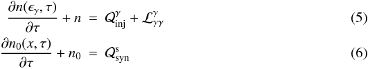 and
and 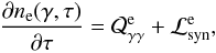 (7)where n, n0 and, ne are the differential γ-ray, soft photon, and electron number densities, respectively, and ϵγ, x, and γ are the corresponding energies normalized in mec2 units. The densities refer to the number of particles contained in a volume element σTR. In other words, if
  expresses the number of particles of species i per ergs per cm3, then
 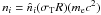 . Time is normalized with respect to the photon crossing/escape time from the source, tcr = R/c. Thus, τ, which appears in the kinetic equations, is dimensionless and equals
  . The operators
  and ℒ denote injection and losses, respectively. The only processes that we take into account are γγ annihilation and synchrotron cooling of the produced pairs. The synchrotron emissivity is approximated by a δ-function, i.e., js(x) = j0δ(x − ϵ0), where ϵ0 = bγ2 is the synchrotron critical energy. In all cases we will assume a monoenergetic γ-ray injection at energy ϵγ.
2.2.1. δ-function approximation for the σγγ cross section
First we will examine the stability of the system using the simplest form for the photon-photon annihilation cross section (Zdziarski & Lightman 1985): 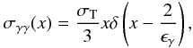 (8)where x,ϵγ are the energies of the soft and γ-ray photons, respectively. The particle injection and loss operators take the following forms:
 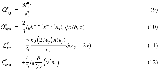 and
and  (13)because each photon-photon annihilation results in a pair of leptons, each one with approximately half of the initial γ-ray energy. In the above equations the “magnetic compactness” was introduced
  (14)The system of Eqs. (5)–(7) can now be written as
 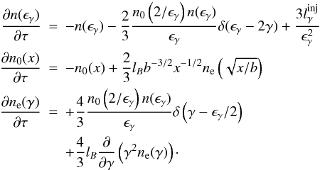 (15)In this section we will examine the stability of the trivial stationary solution of the system (15):
 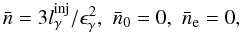 (16)which corresponds to the free propagation of γ-ray photons through the source. To investigate the stability of the system, we assume that initially arbitrarily small perturbations of the soft photon
  and electron
  densities are present, which lead to the perturbation of the γ-ray photon density n′. After linearization, the system (15) becomes
 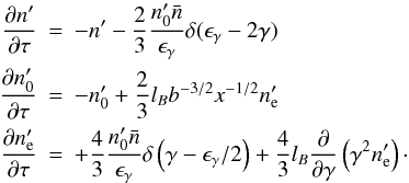 (17)The stability analysis of the system above can be simplified when one works with the Laplace transformed number densities:
 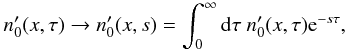 (18)with s being the solution to the eigenvalue problem:
 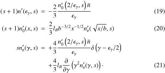 For large τ both the soft photon and electron distributions behave as esτ. If s = −1, then
  and the γ-ray photons freely escape from the source. If s > 0, one finds solutions that grow with elapsing time. The marginally stable solution, which is obtained when one sets s = 0, will be examined below.
Combining Eqs. (19)–(21) leads to an ordinary differential equation for the perturbed electron distribution with the following solution: 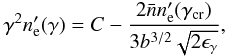 (22)where
  . Setting γ = γcr in the above equation one finds
 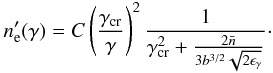 (23)Then the perturbed photon distribution is found using Eq. (20).
As already mentioned in Sect. 2.1, the γ-ray compactness cannot become arbitrarily high but instead saturates at a critical value  . When
  only a negligible fraction of the hard photon luminosity will be absorbed, i.e.,
  , or equivalently
  . We call critical the injected luminosity required for
  to occur. After this point any further increase of the injected luminosity will be seen as an increase of the luminosity in soft photons. Using Eqs. (19), (20), and (23) one derives
 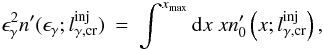 (24)where
  . Solving the above equation with respect to , we find
 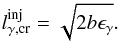 (25)To compare our results with the value
  found by SK, who have used catastrophic synchrotron losses, we have to take the following steps:
-
1.
the case of synchrotron cooling degenerates to the“catastrophic losses case” when the threshold energy forabsorption 2/ϵγ equals the maximum soft photon energy xmax;
-
2.
in SK the volume element is defined as V = πR3, whereas we used V = 4/3πR3. Thus, the replacement
 should be made;
 -
3.
finally, in SK the luminosity compactness is not given by the conventional definition, which we adopted, but is multiplied by the energy ϵγ.
Thus, our result should be compared to  . The critical compactness as a function of ϵγ for two values of the magnetic field is shown in Fig. 1. The two crosses mark the values of SK, which completely agree with ours in the limit of catastrophic losses.
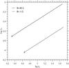 |
Fig. 1 Log-log plot of the critical luminosity compactness |
We note also that Eq. (4), which was obtained by making robust calculations, also agrees with Eq. (25) in the limit of catastrophic losses.
2.2.2. Step function approximation for the σγγ cross section
In this paragraph we analytically find the critical luminosity compactness after adopting a more realistic expression for the annihilation cross section:  (26)where the normalization used is σ0 = 4/3. The initial Eqs. (5)–(7) keep the same form. Only the operator of photon losses becomes
  (27)Following the same steps as those described in Sect. 2.2.1, we find for s = 0
  (28)where
  and γmax = ϵγ/2. Equation (28) can be solved iteratively when writing
  as a sum of approximations, i.e.,
  . Assuming for the first approximation the form n(0) = Cγ-2, we find the other terms of the series expansion:
  where
where  and |λ| < 1 for typical values of the parameters. Thus, the series of approximations converges and can be found in closed form:
  (31)The luminosity in soft and hard photons can then be found
  (32)
(32) (33)The critical γ-ray compactness is given by
 ![Mathematical equation: \begin{eqnarray} \label{lcr_theta} \lcr= \frac{b^2\eg^2}{2 \sigma_0}\left[\left(\frac{b \eg}{2}\right)^{3/2}-\frac{8}{\eg^3}\right]^{-1} \cdot \end{eqnarray}](/articles/aa/full_html/2011/08/aa16763-11/aa16763-11-eq107.png) (34)Figure 2 shows as a function of ϵγ for two values of the magnetic field. When the threshold energy for absorption 2/ϵγ is much lower than the maximum energy of the soft synchrotron photons
(34)Figure 2 shows as a function of ϵγ for two values of the magnetic field. When the threshold energy for absorption 2/ϵγ is much lower than the maximum energy of the soft synchrotron photons  , the critical compactness as a function of ϵγ behaves as for the δ-function cross section. However, when the two energies become comparable, abruptly increases, because the number of soft photons serving as targets for the absorption significantly decreases. This effect can be seen in Fig. 2 as a change in the curvature of the curves.
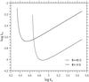 |
Fig. 2 Log-log plot of the critical luminosity compactness |
3. Numerical approach
To numerically investigate the properties of quenching, one needs to solve again the system of Eqs. (5)–(7) augmented to include more physical processes. As in the numerical code, there is no need to treat the time-evolution of soft photons and γ-rays through separate equations, the system can be written:  (35)and
  (36)where ne and nγ are the differential electron and photon number density, respectively, normalized as in Sect. 2. Here we considered the following processes: (i) photon-photon pair production, which acts as a source term for electrons (
 ) and a sink term for photons (
 ); (ii) synchrotron radiation, which acts as a loss term for electrons (
 ) and a source term for photons (
 ); (iii) synchrotron self-absorption, which acts as a loss term for photons (
 ); and (iv) inverse Compton scattering, which acts as a loss term for electrons (
 ) and a source term for photons (
 ). In addition to the above, we assume that γ-rays are injected into the source through the term (
 ). The functional forms of the various rates have been presented elsewhere – Mastichiadis & Kirk (1997) and Petropoulou & Mastichiadis (2009). The photons are assumed to escape the source in one crossing time, therefore tγ,esc = R/c.
The parameters of the problem are completely specified once the values of radius R and of the magnetic field B are set and the injection rate is specified. Because is readily related to the injected luminosity through the relation  (37)where V is the volume of the source, the injection rate is specified once the injection compactness
  and the functional dependence of on ϵγ is set. The electron physical escape timescale from the source te,esc is another free parameter which, however, is not important in our case. Thus, we will fix it at value te,esc = tγ,esc = R/c. The final settings are the initial conditions for the electron and photon number densities. Because we are investigating the spontaneous growth of pairs and synchrotron photons, we assume that at t = 0 there are no electrons or photons in the source, so we set ne(γ,0) = nγ(x,0) = 0.
3.1. Monoenergetic γ-ray injection
As a first example we study the case where the γ-rays injected are monoenergetic at an energy ϵγ. The expected trivial solution of the kinetic equations is that because there are no soft photons in the source, the injected γ-rays will freely escape and their spectrum upon escape will simply be their production one. Electrons and photons at energies different from ϵγ will remain at their initial values, i.e., ne(γ,t) = nγ(x,t) = 0.
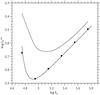 |
Fig. 3 Critical γ-ray compactness as a function of ϵγ when (i) σγγ and synchrotron emissivity are approximated by a Θ- and a δ-function respectively; and (ii) when for both quantities the full expressions are used. For the first case the numerical result (points) and the analytical one given by Eq. (34) (solid line) are shown. The full problem can only be treated numerically and the corresponding result is shown with a dashed line. The size of the source is R = 3 × 1016 cm and the magnetic field strength B = 3.57 G. |
Before numerically examining the stability of the above system using the full expressions for the photon-photon annihilation cross section and the emissivities, we perform a test by comparing the analytical result given by Eq. (34) with the respective numerical. The two solutions completely agree as shown in Fig. 3. In the same figure we also plot the critical γ-ray compactness found numerically when all quantities used were given by their full expressions. The qualitative behaviour of the full problem solution is quite well reproduced by the analytical one obtained while using the Θ- and δ-approximations for the cross section and synchrotron emissivity respectively. This allows us to use the analytical expression given by Eq. (34) for the full problem as well, when investigating the properties of quenching at least qualitatively. From this figure it becomes apparent that γ-ray quenching can affect all photons with energies that satisfy the feedback condition. Starting around this energy and moving progressively to higher ones, we find that the critical compactness first sharply decreases until it reaches a minimum and then starts increasing again, as  asymptotically. The exact value of the critical compactness also depends on the strength of the magnetic field. For a higher B-field the required minimum energy ϵγ decreases, which can be easily deduced by Eq. (2). Note also that because of the marginal relation (34), the required critical injected compactness becomes higher. Thus, by increasing B, the corresponding curve is shifted towards lower γ-ray energies and higher critical compactnesses, keeping its shape (see e.g. Fig. 2).
Figure 4 depicts the results of a series of runs where we kept ϵγ constant and varied . For sufficiently low values of the latter parameter, all γ-rays indeed escape from the system without any impedance. If we call  the compactness of the outgoing radiation at energy ϵγ, then obviously, in this case,
  , where
  is the compactness of the outgoing luminosity. However, above a critical value of , which we will call
  , the loop described above starts operating, transferring the γ-ray luminosity to softer radiation. Thus, for
  , we get
  because saturates – by
  we denote the compactness of the reprocessed luminosity, which appears at lower energies. This can be seen in Fig. 4, where the dashed line curve represents , the dotted line and the full line , which is always equal to because there are no sinks of photons present. For the particular example shown in Fig. 4, the values of the other parameters used are, R = 3 × 1016 cm, B = 40 G and ϵγ = 2.3 × 10⁴.
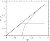 |
Fig. 4 Plot of the compactness of emerging hard |
 |
Fig. 5 Multiwavelength spectrum for a choice of |
Figure 5 shows the multiwavelength (MW) spectrum for the particular value of , which results in equipartition between soft and hard luminosities, i.e.,  . While the hard luminosity is simply the escaping monoenergetic radiation at ϵγ, the soft spectrum mainly consists of the synchrotron component produced from the secondary pairs, which were injected at energies γp = γe = ϵγ/2. The peak of this component is at
  , while it has a spectral index of − 1/2 (or + 1/2 in νFν units) as a result of the electron cooling to a γ-2 distribution below the energy of injection. There is also a synchrotron self-Compton (ssc) component, which is greatly suppressed by Klein-Nishina effects. As can be seen from the figure, the corrections introduced from the inclusion of inverse Compton scattering and synchrotron self-absorption are negligible, at least for our set of parameters.
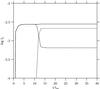 |
Fig. 6 Time evolution of the soft |


Figure 6 shows the time evolution of the different luminosity compactnesses for the example case presented in Fig. 5. Although the dynamical, non-linear system of equations describing the system (see for example system of Eq. (15)) is of third order, which in principle can lead to unstable solutions or/and “chaotic” behaviour (SK), the system quickly reaches a stable state after a few crossing times. Figure 6 shows that although initially absent, a soft photon population builds up, which leads to a decrease of  , because γ-rays are being absorbed by the soft photons.
3.2. Power-law injection
As a next step we investigate the effects of quenching for a power-law injection of γ-rays, i.e., when the injection rate can be written as  (38)where Q0 is a normalization constant depending on the value of α, the low- and high- energy cutoffs of the distribution.
Before proceeding to more quantitative calculations, we remark that obviously, for a given B the feedback criterion for quenching to start will be that of Eq. (2) where ϵγ should be replaced by ϵγmax. Assuming that this condition holds and that the compactness of the γ-rays is above the critical one, the production of synchrotron photons with energy  is guaranteed. This means that γ-rays with energy ϵγ ≳ ϵγmin,eff should interact in γγ interactions, where
 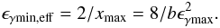 (39)Thus, depending on the relation between ϵγmin,eff and ϵγmin we can distinguish two cases:
-
(i)
ϵγmin < ϵγmin,eff: in this case quenching will affect γ-rays from ϵγmax down to ϵγmin,eff. For ϵγ ≤ ϵγmin,eff the spectrum will be unaffected, i.e., it will be the same as the one at injection.
-
(ii)
ϵγmin,eff < ϵγmin: in this case quenching will affect the whole γ-ray spectrum.
The above two cases are exemplified in Figs. 7 and 8. In both figures we assumed that γ-rays with a power-law form of slope α = 2 are injected in a source of radius R = 3 × 1016 cm and magnetic field strength B = 40 G. The only difference between the two cases is in the lower and upper limits, which are ϵγmin = 23 and ϵγmax = 2.3 × 10⁴ for the case shown in Fig. 7 and ϵγmin = 230 and ϵγmax = 2.3 × 10⁵ for the case shown in Fig. 8.
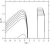 |
Fig. 7 MW spectra for a power-law injection of γ-rays of the form |

In the case of Fig. 7 we have ϵγmin < ϵγmin,eff = 1.7 × 10⁴ and, as can be seen from the figure, the power-law breaks above ϵγmin,eff because of quenching – indeed, we find that the value of ϵγmin,eff is in reality lower by a factor of 2 than the one given in Eq. (39), because in the numerical calculations shown here we use the full expressions for the synchrotron emissivity and the cross-section for γγ and not the δ-function approximations implied in the derivation of the above relation. It is interesting to note that as the γ-ray luminosity increases and thus the quenching becomes more effective, the break between the unabsorbed and absorbed part of the power-law becomes more abrupt.
In the case of Fig. 8, on the other hand, the choice of the parameters were such as to make ϵγmin,eff comparable to ϵγmin. Thus, according to the qualitative analysis presented above, quenching should affect the whole γ-ray distribution. Indeed, as can be deduced from the figure, as the luminosity increases, absorption is moving progressively to lower γ-ray energies, until it affects the whole distribution.
 |
Fig. 8 Same as in Fig. 7 with ϵγmin = 2.3 × 10² and ϵγmax = 2.3 × 10⁵ with Q0 starting from Q0 = 2.5 × 10⁻⁴. |
We also investigated the relation between the slope of the injected (αinj) and the “quenched” (αque) γ-ray spectrum. For that reason, we ran the code for different αinj, choosing each time suitable values of the source parameters to enable quenching. Figure 9 shows the result of the runs (solid line) and the slope αinj + 1 (dashed line) for comparison reasons. We find that  . Thus, quenching becomes more pronounced as the injected spectrum gets steeper.
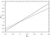 |
Fig. 9 Slope of the quenched γ-ray spectrum as a function of the injected spectrum’s slope (solid line). To facilitate a comparison the line αinj + 1 is also shown (dashed line). |
4. Application to the one-zone homogeneous models: the 3C 279 case
The above has a straightforward application to the so-called one-zone homogeneous models, which are customarily used to fit the MW spectra of Active Galactic Nuclei (AGN) (Böttcher et al. 2009; Aleksić et al. 2011). According to these models, the “source” contains electrons and/or protons, which radiate through various processes and form a spectrum that can then be fitted to the observed data by varying certain key parameters – for a detailed description see Mastichiadis & Kirk (1997) and Konopelko et al. (2003).
Alternatively, one can assume that the γ-rays are produced by some mechanism and investigate the parameter space that allows the escape of these γ-rays. To perform this analysis, one does not require the existence of other softer photons that act as targets, but one simply has to look for the threshold conditions for photon quenching. In other words, the relevant question one has to ask is: assume a spherical source of radius R containing a magnetic field B and producing a γ-ray spectrum that is measured at Earth with a flux Fγ(ϵγ). If the source is moving with a Doppler factor δ with respect to us, what is the parameter space of R, B, and δ that allows the γ-rays to escape? As we will show, this can give very robust lower limits for the Doppler factor δ.
The luminous quasar 3C 279 is a good example. A recent comprehensive review of observations can be found in Böttcher et al. (2009). Here we will mainly focus on the 2006 campaign, which discovered the source at VHE γ-rays, showing a high TeV flux (MAGIC Collaboration et al. 2008), while the X-rays were at a much lower level.
To apply the ideas discussed in the previous section, we follow the procedure below.
We assume a spherical source of radius R moving with Doppler factor δ with respect to us and containing a magnetic field of strength B. We assume that γ-rays are produced by some unspecified mechanism inside the source and, upon escape, they form the observed γ-ray spectrum. If is the compactness of the γ-rays (cf. Eq. (1)), we can relate it to the observed integrated flux  by the relation
 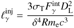 (40)where DL = 3.08 Gpc is the luminosity distance to the source. Here we used a cosmology with Ωm = 0.3, ΩΛ = 0.7 and H0 = 70 km s-1 Mpc-1.
To model the TeV emission, we performed a χ2 fit to the MAGIC data, corrected for intergalactic γγ absorption (Böttcher et al. 2009), of the form νFν = Aν − α for  where A = 1.3 × 1031 Jy Hz, α = 0.7,
  Hz and
  Hz. Then we injected γ-rays in the code of the form
  for ϵγmin < ϵγ < ϵγmax where the normalization is set by condition (37) with the integration taking place between
 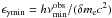 and
and 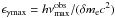 .
.
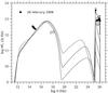 |
Fig. 10 MW spectra of 3C 279 for R = 1016 cm, B = 40 G and δ = 100.8 (dotted line), 101.0 (dashed line), 101.2 (dot-dashed line) and 101.4 (solid line). In all cases the γ-ray injection would have produced the solid line in the absence of quenching. Black squares and bowtie represent the observational data from February 2006. |
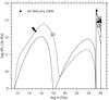 |
Fig. 11 MW spectra of 3C 279 for R = 1016 cm, δ = 101.2 and B = .16 G (solid line), 1.6 G (dashed line) and 16 G (dotted line). In all cases the γ-ray injection would have produced the solid line in the absence of quenching. Black squares and bowtie represent the observational data from February 2006. |
Figure 10 depicts the resulting MW spectra for R = 1016 cm, B = 40 G and δ varying between 100.8 to 101.4 with increments of 0.2 in the exponent. Only the run with the highest value of δ can fit the TeV data. The other three, even though they have parameters that could also fit the data, they do not because of quenching. It is important to repeat at this point that the γ-ray luminosity produced in these cases is the maximum possible that the system can radiate for the particular choice of R, B, and δ. Any effort to increase the γ-ray flux by e.g. increasing would only result in an increase of the reprocessed radiation.
Figure 11 depicts a series of similar runs with R = 1016 cm, δ = 101.2 and B = .16 G (solid line), B = 1.6 G (dashed line) and B = 16 G (dotted line). While for low B values there is no quenching, this begins to appear at higher values of the magnetic field. Note, however, that the value of B = 1.6 G produces an acceptable fit, because the soft reprocessed radiation does not violate any observable limit (most notably the X-rays) and it can produce a marginally acceptable fit to TeV γ-rays. Based on this, one can define a limiting value of the magnetic field Bq,mx(R,δ) with the property that if B > Bq,mx, the quenching does not allow the internally produced γ-ray luminosity to escape. Therefore Bq,mx is the highest allowed value that the B-field can take for the observed flux of TeV γ-rays.
Figure 12 depicts the locus Bq,mx as a function of the size of the source R for various Doppler factors δ. Each line separates the parameter space into two regions: because of the quenching, a choice of R and B above the locus produces a far too low γ-ray flux that cannot fit the TeV observations. For example, if one assumes that δ = 10 and R = 2.5 × 1016 cm – so that it corresponds to a variability timescale of 1 day, the magnetic field cannot exceed 0.3 G. However, owing to the steep dependence of the flux on δ (cf. Eq. (40)), the above condition is greatly relaxed for higher values of δ.
We should also mention that Bq,mx not only depends on δ and R, but also on the upper cutoff ϵγmax of the injected power-law in γ-rays. For the calculations performed here, we chose ϵγmax such as to match the highest observed frequency in the data set, i.e., 1026 Hz. If one assumes that the internally produced γ-rays can extend to even higher energies, then the value of Bq,mx is affected as well. Accordingly we found that if we were to repeat the same calculations with ϵγmax ten times higher than the value we used, then quenching would affect the flux more and the lines of Fig. 12 would have to shift upwards by a factor of 2. Therefore, Fig. 12 can be taken as a conservative lower limit on Bq,mx.
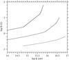 |
Fig. 12 Parameter space of the allowed values of the magnetic field B as a function of the size of the source R for Doppler factors of δ = 10 (dotted line), 15.8 (dashed line), and 25 (solid line). The space above a line for a certain δ corresponds to combinations of R and B that cannot successfully fit the TeV observations of 3C 279. |
5. Summary and discussion
We have examined the effects of photon quenching on compact γ-ray sources. Automatic photon quenching, first proposed by SK, is a non-linear network of two processes that are very common in high-energy astrophysics, namely photon-photon annihilation and lepton synchrotron radiation. We verified and expanded both analytically and numerically the results of SK and we showed that this network, when applied to compact γ-ray sources, can give limits on the Doppler factor, which depend on the source radius and on the magnetic field strength only. This is a theoretically derived limit and as such does not depend on the soft photon populations that might be present inside the source.
It is important to note that photon quenching can be investigated only when the radiation transfer problem is solved self-consistently because it is a non-linear process that involves redistribution of energy from the γ-rays to the lower energy parts of the photon spectrum. For this we used a system of kinetic equations that treats in the simplest case γ-ray annihilation and electron synchrotron radiation. Using suitable δ-function approximations for the photon-photon annihilation cross section and for the photon synchrotron emissivity, we were able to verify the results of SK in the limit where synchrotron losses can be considered as catastrophic (see Fig. 1). On the other hand, using a more realistic step function for the cross section, we were able to find a very good agreement with numerical results, which utilized the full photon-photon annihilation cross section. Furthermore, we extended our numerical study in the case where γ-rays are injected in the form of a power-law. We found that quenching can be responsible for wide spectral breaks, which become more pronounced as the injected γ-rays become steeper (see Fig. 9).
Quenching has some interesting consequences when applied to existing γ-ray sources. For example, for the 2006 MAGIC observations of the quasar 3C 279, modelling with combinations of low values of the Doppler factor δ and high values of the magnetic field strength B lead to strong absorption of the injected γ-rays. The only way to avoid quenching is either to assume typical values of δ (i.e., around 10) and low values of B or, alternatively, high values for both δ and B – see Fig. 12.
We restricted our analysis to cases where γ-rays are injected into the source without being too specific in assigning a particular radiation mechanism for producing them. We preferred this approach because our aim was to calculate the effects of quenching using simple functional forms for the γ-rays and not to model the source in detail. For example, we could have used proton synchrotron radiation to fit the 3C 279 TeV observations. However, this would have involved extra parameters for the radiating relativistic protons and would have complicated the analysis beyond the level at which we would like to present it here.
In our analytical treatment we ignored inverse Compton scattering, because its inclusion would have complicated the analysis. On the other hand, it was taken into account in all our numerical calculations, although it is greatly suppressed by Klein-Nishina effects (see Fig. 5). This process can still make an impact in cases where the soft photon compactness greatly exceeds the magnetic one (cf. Eq. (14)). However, this has to be seen in conjunction with the overall fitting of the MW spectrum of the source and we avoided presenting it here, although we took it into account in Sect. 4 when performing the analysis on quasar 3C 279.
Concluding, quenching has many far-reaching implications for the modelling of compact γ-ray sources such as Active Galactic Nuclei and Gamma Ray Bursts. Because quenching operates in an autoregulatory manner by coupling electrons to photons, its effects on the photon spectra cannot be manifested if the modelling is done by assuming an ad-hoc radiating electron and/or proton distribution. This could lead to parameter choices that lie within the quenching “forbidden” parameter space, making them in essence invalid.
On the other hand, if taken fully into account, quenching can give robust limits for important source parameters such as its size, magnetic field, and the Doppler factor for a given γ-ray flux. In the case of 3C 279 for example, we found that to avoid quenching, the source should have a large Doppler factor (δ ≳ 10) whenever high B values are adopted. Similar constraints could be found for other AGNs with spectra extending to even higher energies (~1–10 TeV). In these cases the conditions for quenching are more stringent, because they critically depend on the maximum energy of the γ-ray photons and are certainly worth investigating further.
We note that in the same framework an analogous study where ultrarelativistic protons are the primary injected particles has earlier been presented by Kirk & Mastichiadis (1992).
Acknowledgments
We would like to thank Dr. John Kirk for useful comments and discussion. This research has been co-financed by the European Union (European Social Fund – ESF) and Greek national funds through the operational Program “Education and Lifelong Learning” of NSRF – Research Funding Program: Heracleitus II.
References
- Aleksić, J., Antonelli, L. A., Antoranz, P., et al. 2011, A&A, 530, A4 [NASA ADS] [CrossRef] [EDP Sciences] [Google Scholar]
- Bonometto, S., & Rees, M. J. 1971, MNRAS, 152, 21 [NASA ADS] [Google Scholar]
- Böttcher, M. 2007, Ap&SS, 309, 95 [NASA ADS] [CrossRef] [Google Scholar]
- Böttcher, M., & Chiang, J. 2002, ApJ, 581, 127 [NASA ADS] [CrossRef] [Google Scholar]
- Böttcher, M., Reimer, A., & Marscher, A. P. 2009, ApJ, 703, 1168 [NASA ADS] [CrossRef] [Google Scholar]
- Coppi, P. S. 1992, MNRAS, 258, 657 [NASA ADS] [CrossRef] [Google Scholar]
- Guilbert, P. W., Fabian, A. C., & Rees, M. J. 1983, MNRAS, 205, 593 [NASA ADS] [CrossRef] [Google Scholar]
- Herterich, K. 1974, Nature, 250, 311 [NASA ADS] [CrossRef] [Google Scholar]
- Jelley, J. V. 1966, Nature, 211, 472 [NASA ADS] [CrossRef] [Google Scholar]
- Kataoka, J., Takahashi, T., Makino, F., et al. 2000, ApJ, 528, 243 [NASA ADS] [CrossRef] [Google Scholar]
- Katarzyński, K., Ghisellini, G., Tavecchio, F., et al. 2005, A&A, 433, 479 [NASA ADS] [CrossRef] [EDP Sciences] [Google Scholar]
- Kazanas, D. 1984, ApJ, 287, 112 [NASA ADS] [CrossRef] [Google Scholar]
- Kirk, J. G., & Mastichiadis, A. 1992, Nature, 360, 135 [NASA ADS] [CrossRef] [Google Scholar]
- Konopelko, A., Mastichiadis, A., Kirk, J., de Jager, O. C., & Stecker, F. W. 2003, ApJ, 597, 851 [NASA ADS] [CrossRef] [Google Scholar]
- MAGIC Collaboration, Albert, J., Aliu, E., Anderhub, H., et al. 2008, Science, 320, 1752 [NASA ADS] [CrossRef] [PubMed] [Google Scholar]
- Mastichiadis, A., & Kirk, J. G. 1995, A&A, 295, 613 [NASA ADS] [Google Scholar]
- Mastichiadis, A., & Kirk, J. G. 1997, A&A, 320, 19 [NASA ADS] [Google Scholar]
- Petropoulou, M., & Mastichiadis, A. 2009, A&A, 507, 599 [NASA ADS] [CrossRef] [EDP Sciences] [Google Scholar]
- Stawarz, Ł., & Kirk, J. G. 2007, ApJ, 661, L17 [NASA ADS] [CrossRef] [Google Scholar]
- Stern, B. E., Begelman, M. C., Sikora, M., & Svensson, R. 1995, MNRAS, 272, 291 [NASA ADS] [CrossRef] [Google Scholar]
- Svensson, R. 1987, MNRAS, 227, 403 [NASA ADS] [Google Scholar]
- Zdziarski, A. A., & Lightman, A. P. 1985, ApJ, 294, L79 [NASA ADS] [CrossRef] [Google Scholar]
All Figures
|
Fig. 1 Log-log plot of the critical luminosity compactness |
| In the text | |
|
Fig. 2 Log-log plot of the critical luminosity compactness |
| In the text | |
|
Fig. 3 Critical γ-ray compactness as a function of ϵγ when (i) σγγ and synchrotron emissivity are approximated by a Θ- and a δ-function respectively; and (ii) when for both quantities the full expressions are used. For the first case the numerical result (points) and the analytical one given by Eq. (34) (solid line) are shown. The full problem can only be treated numerically and the corresponding result is shown with a dashed line. The size of the source is R = 3 × 1016 cm and the magnetic field strength B = 3.57 G. |
| In the text | |
|
Fig. 4 Plot of the compactness of emerging hard |
| In the text | |
|
Fig. 5 Multiwavelength spectrum for a choice of |
| In the text | |
|
Fig. 6 Time evolution of the soft |
| In the text | |
|
Fig. 7 MW spectra for a power-law injection of γ-rays of the form |
| In the text | |
|
Fig. 8 Same as in Fig. 7 with ϵγmin = 2.3 × 10² and ϵγmax = 2.3 × 10⁵ with Q0 starting from Q0 = 2.5 × 10⁻⁴. |
| In the text | |
|
Fig. 9 Slope of the quenched γ-ray spectrum as a function of the injected spectrum’s slope (solid line). To facilitate a comparison the line αinj + 1 is also shown (dashed line). |
| In the text | |
|
Fig. 10 MW spectra of 3C 279 for R = 1016 cm, B = 40 G and δ = 100.8 (dotted line), 101.0 (dashed line), 101.2 (dot-dashed line) and 101.4 (solid line). In all cases the γ-ray injection would have produced the solid line in the absence of quenching. Black squares and bowtie represent the observational data from February 2006. |
| In the text | |
|
Fig. 11 MW spectra of 3C 279 for R = 1016 cm, δ = 101.2 and B = .16 G (solid line), 1.6 G (dashed line) and 16 G (dotted line). In all cases the γ-ray injection would have produced the solid line in the absence of quenching. Black squares and bowtie represent the observational data from February 2006. |
| In the text | |
|
Fig. 12 Parameter space of the allowed values of the magnetic field B as a function of the size of the source R for Doppler factors of δ = 10 (dotted line), 15.8 (dashed line), and 25 (solid line). The space above a line for a certain δ corresponds to combinations of R and B that cannot successfully fit the TeV observations of 3C 279. |
| In the text | |
Current usage metrics show cumulative count of Article Views (full-text article views including HTML views, PDF and ePub downloads, according to the available data) and Abstracts Views on Vision4Press platform.
Data correspond to usage on the plateform after 2015. The current usage metrics is available 48-96 hours after online publication and is updated daily on week days.
Initial download of the metrics may take a while.