| Issue |
A&A
Volume 532, August 2011
|
|
|---|---|---|
| Article Number | A70 | |
| Number of page(s) | 9 | |
| Section | Astrophysical processes | |
| DOI | https://doi.org/10.1051/0004-6361/201016289 | |
| Published online | 25 July 2011 | |
Solar coronal magnetic field diagnostics through polarimetric forward modelling of the Hanle effect
Dipartimento di Fisica e Astronomia, SASSUniversità degli Studi di Firenze, Largo E. Fermi 2, 50125 Firenze, Italy
e-mail: This email address is being protected from spambots. You need JavaScript enabled to view it.
Received: 9 December 2010
Accepted: 1 June 2011
Abstract
Context. Progress in the solution to some of the most outstanding open problems of solar physics, such as coronal heating, solar wind acceleration, the generation and triggering of explosive events like flares and CMEs, hinges on the provision of a more stringent estimate of the solar magnetic field coordinates.
Aims. We seek a way to infer the magnetic field of the solar atmosphere. A very promising way of doing this is by using the Hanle effect in resonance scattering in the Lα line of the solar atmosphere.
Methods. By forward modelling the known scattering effects in the presence of magnetic fields, i.e. rotation of the plane of polarisation and depolarisation of the linear polarisation parameters, and by comparing them to observations, one could potentially uncover the magnetic morphology and restrict its intensity range. We simulate the effects of simple dipole configurations along the coordinate axes and analyse the outcome through two kinds of graphs (i.e. the difference in angle of the plane of linear polarisation with respect to the field-free case, and the relative depolarisation).
Results. The graphs are either symmetric, anti-symmetric or asymmetric with respect to the (y,z) plane. This is explained by invoking two symmetry operations and taking into account that the magnetic field is a pseudovector. We also show the polarimetric effects of active regions and use them pairwise with the magnetic field due to dipoles to analyse the polarimetric signatures of magnetic field line loops. Inspired by the famous TRACE image, we finally show what one could expect from polarimetry performed on the region of the solar atmosphere displayed in the image.
Conclusions. By combining the two complementary remote sensing techniques, i.e. the Zeeman and the Hanle effect, in all thinkable ways with tracers such as the images revealed by TRACE, SOHO, STEREO, etc., we hope one day to be able to infer the solar magnetic field coordinates. Much theoretical and instrumental work still lies ahead, however.
Key words: polarization / scattering / Sun: corona / Sun: magnetic topology
© ESO, 2011
1. Introduction
The technological revolution and the accompanying advent of space missions in the last half century have unveiled a myriad of strange and exotic phenomena hitherto unknown in the field of astrophysics and astronomy. Just to mention a few, these include neutron stars, indirect evidence of black holes, AGNs, accretion discs, GRBs, ultra-high energy cosmic rays etc. In terms of our own Sun, the discoveries include the existence of a slow and fast solar wind, a million-degree hot outer solar atmosphere, known as the solar corona, and subsequent emission of X-rays, prominences, flares, and CMEs. These solar phenomena are all without exception thought to have the solar magnetic field as their main player, and arise from the solar magnetic field’s highly intricate, complex, and unfortunately still not well-understood interaction with the solar plasma. Solar theoretical physicists have come up with very interesting, exciting, and plausible explanations and have to some degree succeeded in elucidating the physics at work qualitatively, but the absolute absence of “direct” measurements of the full three-dimensional magnetic field vector remains an obstacle to further development and refinement of these theories. If we do not address this fundamental issue, all of the theories based on it will be destitute of the very pillars on which modern science rests, experimental fact, and it will be very difficult to distinguish between competing theories.
The quantitative determination of the solar coronal magnetic field basically rests upon two remote-sensing techniques for inferring its topology and intensity. These are the Zeeman and Hanle effects. Although very promising and ingenious, these methods still have to be refined, both from a modelling and an instrumental point of view. There are to date only a few measurements of the solar coronal magnetic field.
The Zeeman effect is the splitting up of degenerate atomic energy levels into differently polarised spectral components. Depending on the geometry, one can in some cases infer the magnetic field from the observed linearly and circularly polarised spectral components. Although very effective at photospheric levels, it is difficult to use in the corona because of the high temperatures of the coronal plasma that wipe out the spectral components owing to Doppler broadening. The Zeeman splitting is, however, proportional to the square of the wavelength and can thus be used in some cases as a diagnostic tool for the magnetic field of the corona by analysing emission lines that fall into the visible and especially IR part of the electromagnetic spectrum.
By using the magnetograph relation and analysis of the “green” 5303 Å Fe xiv line, Harvey (1969) was able to provide an estimate of the upper limit on the longitudinal component of the magnetic field, of about 40 G. Mickey (1973) succeeded in using the same line to measure the coronal field direction, and later House (1977) calculated and Querfeld (1977) observed how the linear polarisation of the 10747 Å Fe xiii line is quite sensitive to the coronal magnetic field orientation, leading Lin et al. (2000) to measure the magnetic flux density along a single LOS above an active region of about 30 G. More recently, Lin et al. (2004) have refined their measurement and found a magnetic flux density along the LOS of about 4 G at a height of roughly 1.1 solar radii.
The Hanle effect is the modification of the polarisation properties of resonance scattering in the presence of a magnetic field. This modification is two-fold; i.e. it entails a rotation of the plane of polarisation and causes a de-or hyper-polarisation of the scattered radiation. Although its detection is achieved by polarimetric observations as in the Zeeman case, it has two very attractive advantages over the Zeeman effect. This is, on the one hand, its sensitivity to the magnetic field, which depends on the ratio of the upper levels Zeeman splitting to its inverse lifetime, making it sensitive to fields in the range from ~0.1 G to ~100 G, and on the other hand, its independence of the Doppler broadening of the line, converting it, together with the complementary Zeeman effect, into the method for scrutinising coronal magnetic fields.
The inspiration for this paper comes from some important contributions to the Hanle effect and its applications to astrophysics. We will simply mention the most important, referring the interested reader to a more thorough discussion that can be found in the introduction of a previous paper, Khan et al. (2011), hereafter Paper I. They include Hanle (1924) for uncovering the laws of resonance scattering in the presence of a magnetic field, Öhman (1929) for proposing the Hanle effect for magnetic field diagnostics of solar prominences, Bommier & Sahal-Bréchot (1982) for working out the full quantum mechanical theory of resonance scattering in the presence of magnetic fields for the 1216 Å Lα line and for suggesting it as a means of diagnosing the coronal magnetic field after a line-of-sight (LOS) integration of its emissivity, Fineschi et al. (1993) for a first implementation of a LOS integration of the Lα line and for a thorough discussion of the feasibility of actually using LOS-integrated information for magnetic field diagnostics both from theoretical and experimental points of view. For LOS-integrated simulations using the first few lines of the Lyman-series, see Fineschi et al. (1991, 1992, 1999), Raouafi et al. (2009), Derouich et al. (2010), and Judge et al. (2006) using forbidden emission lines.
It is our firm view that one very powerful way of improving the current situation faced by solar physicists in determining the solar coronal magnetic field, is by simulating the polarimetric effects of a wide variety of magnetic structures present in the solar corona, thus leading to a deeper understanding of the Hanle effect in forward modelling and, at the same time, enabling ourselves to be fully equipped for correctly interpreting the observational data once it becomes available. In Paper I we have exclusively shown global graphs of the polarimetric outcome due to three polarimetrically active agents, that is, magnetic fields, non-radial velocities (solar wind), and anisotropies in the radiation field because of the presence of active regions on the solar surface, using a self-consistent 2.5-D axisymmetric MHD model of the solar corona representing solar minimum conditions. The results were very revealing in that they, on the one hand, showed the relative contributions from each of the three agents for a self − consistent coronal model and, on the other hand, where to expect them.
In the present paper, however, our main goal is to forward-model the effects of coronal magnetic structures due to active regions in an isolated fashion by taking snapshots of small local, magnetically infested regions and by reporting on the Stokes parameters obtained. After having gone through a number of examples, we try in the end to answer the extremely crucial question of the usefulness of this method for magnetic field diagnostics. Are the results degenerate, i.e., does the knowledge of the linear polarisation parameters of a given region of the solar corona unequivocally reveal the magnetic structures that gave rise to it?
In Sect. 2 we present the coronal and magnetic models, and in Sect. 3 we show and discuss our simulation results. Finally in Sect. 4 we draw our conclusions and comment on future developments.
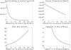 |
Fig. 1 The solar coronal thermodynamic model. |
2. The coronal and magnetic models
We have chosen to work with a spherically symmetric model of the corona, shown in Fig. 1. In the bottom right hand panel, we show the logarithm of the ratio of the density of hydrogen atoms to the density of protons as a function of the logarithm of the temperature, which gives the density of hydrogen atoms with the information contained in the first two graphs as a function of the radial distance from the Sun’s surface.
For the details on the theory of resonance scattering and the Hanle effect and an explanation of the model atom used, we refer the reader to Sect. 2 of Paper I. Following the analysis of instrumental requirements presented in Sect. 4 of that paper, we restrict ourselves to the Lα line, simply because it is one of the most promising, if not the most promising line for polarimetry of the solar corona, because it is one of the brightest lines and, most important for polarimetry, almost exclusively excited radiatively (Gabriel et al. 1971).
The coronal magnetic field is thought to be responsible for much of the varied phenomenology encountered at a distance of 1.1 solar radii1, such as polar plumes, coronal holes, helmet streamers, prominences, flares, and CMEs, and the ultimate goal for polarimetry is to uncover their polarimetric signatures. Inspired by the intriguing image in Fig. 2 made by TRACE, we focus in this paper on polarimetry of active regions, that is, regions of the solar atmosphere in which the intensity of the magnetic field is particularly high and thought to be the breeding ground for solar activity in the form of solar flares and CMEs. The way to go about simulating these active regions is by placing one or more magnetic dipoles right beneath the solar surface at 0.9 solar radii and varying their orientation. The magnetic field-line loops’ foot points form active regions and these have the effect of enhancing the chromospheric Lα radiation diffused by the corona with respect to the “quiet” surroundings, (see discussion in Sect. 2.4 of Paper I). We will thus study the polarimetric signature induced by dipolar magnetic fields and by this radiation enhancement effect of active regions, first separately and then together.
Superposing a magnetic field on a pre-existing hydrodynamic coronal model is somewhat inconsistent, since one neglects the back reaction from the magnetic field on the plasma and vice versa. Owing to the exploratory nature of our investigation we content ourselves with this way of simulating coronal magnetohydrodynamics, leaving the polarimetry of full 3-D self-consistent coronal models to a later point, in order to check the results obtained with this approximative model.
The type of modelling presented in this and many of the previously mentioned papers is becoming an increasingly common exploration of the coronal appearance in polarisation, mainly as a way to tackle the hideous problem of LOS integrations through a thin magnetised plasma. Unfortunately, however, interpreting LOS-integrated data is inherently a risky business and extreme care is warranted when one attempts to use it for deducing physical observables.
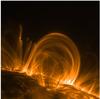 |
Fig. 2 Coronal loops as observed by TRACE in the 17.1 Å Fe ix line. Image credit: TRACE, http://apod.nasa.gov/apod/ap000928.html |
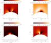 |
Fig. 3 Rotation of the plane of linear polarisation with respect to the field-free case for simulations in which a magnetic dipole has been placed in r = (0,0,0.9) in units of solar radii, with a magnetic moment of m = (1,0,0), upper left, m = (0,1,0), upper right, m = (0, − 1,0), lower left, and m = (0,0,1), lower right, respectively. |
3. Results
The results of the simulations presented in this paper give the line- and LOS-integrated emission coefficients, or Stokes parameters of the area of the plane of the sky under examination. As stated in the introduction, our investigation is two-fold, i.e., on the one hand, to disclose the polarisation parameters corresponding to given localised magnetic structures, and, on the other, to address the crucial question of their uniqueness. To this end we only make use of two of the four Stokes parameters, namely Q and U, the reasons being that the intensity remains almost unaltered in the presence of magnetic fields and that the V Stokes parameter is equal to zero, as a result of the line integration and the fact that the hydrogen atoms are only excited by unpolarised radiation. A very convenient and revealing way to depict the behaviour of the linear polarisation parameters is to define the fractional linear polarisation, PL, given by 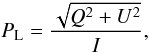 (1)and the polarisation angle, α, given by
 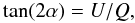 (2)and use these definitions to further define both the relative depolarisation in percent as RD = [(P0 − PL)/P0] ∗ 100%, where P0 is the degree of linear polarisation in the absence of symmetry-breaking effects (magnetic fields, non-radial outflows, presence of active regions), and the rotation angle, Dα, as the difference, measured counterclockwise in degrees, of the polarisation angle with respect to the parallel to the solar limb2. The relative depolarisation graphs are shown in green, whereas the difference in angle between the plane of polarisation and the solar limb are shown in red, and it is through the close inspection of these two kinds of graph, that we learn about how to correlate the polarisation parameters to the magnetic field that gives rise to it and about its possible degeneracy.
3.1. Polarimetry of magnetic configurations due to dipoles oriented along the coordinate axes
With reference to a right-handed coordinate system, (x,y,z), with the plane of the sky represented by the (x,z) plane and the y axis pointing in the observer-Sun direction, we start by showing the effects of the magnetic field from a dipole located at r = (0,0,0.9) in units of solar radii and oriented sequentially along the ± x, y, and z axes, with a magnetic moment of m = (1,0,0), m = (0,1,0), and m = (0,0,1) respectively. The moments are given in units such that the value of the magnetic field at the solar north pole is always 1000 G, corresponding to the “typical” value found in sunspots.
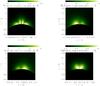 |
Fig. 4 Relative depolarisations for the simulations of magnetic dipoles along the coordinate axes corresponding to Fig. 3. |
Common to all the graphs shown in Figs. 3 − 4 is that the phenomena of rotation and depolarisation take place in the close neighbourhood of the pole, reflecting the rapid fall-off as r-3 of the dipolar field. The graphs due to the dipoles having m = ( − 1,0,0) and m = (0,0, − 1), are not shown since they are degenerate, that is, identical to the upper left and lower right images of Figs. 3 and 4, respectively.
Inspection of Figs. 3 − 4 shows that the graphs are either symmetric (RDs of the dipoles along the x and z axes), antisymmetric (Dαs of the dipoles along the x and z axes), or non-symmetric with respect to the (y,z) plane (Dαs and RDs of the dipoles along the y axes). The antisymmetric Dαs are endowed with alternating, almost artistic lobes that make them seem more a piece of artwork than a simulation of astrophysical reality. The only somewhat “intuitive” aspect of the graphs are the values obtained, which roughly speaking are in line with those obtained by other groups that have done similar simulations: Bommier & Sahal-Bréchot (1982), Fineschi et al. (1991, 1992, 1993, 1999), Raouafi et al. (2009), and Derouich et al. (2010).
The graphs embody the cumulative result of thousands of scattering events along each LOS, and it is, needless to say, neither technically feasible nor desirable to give an exhaustive explanation of their detailed form. It is, however, of utmost interest to explain the symmetries there, since they could prove very valuable for elucidating the magnetic field structure behind the observations.
3.2. Symmetries in Dα and RD graphs for dipole configurations of the magnetic field
The value of the magnetic field at the solar north pole is always 1000 G, and the dipole is always located in r = (0,0,0.9). There are two symmetries that we use in order to predict the results of changing the dipole configuration.
-
S1
-
Anterior-posterior symmetry, followed by a 180 degreerotation about the z axis.
-
-
S2
-
Specular symmetry, that is left right symmetry with respect tothe (y,z) plane.
-
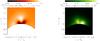 |
Fig. 5 The rotation angle and relative depolarisation for |


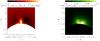 |
Fig. 6 The rotation angle and relative depolarisation for |


The first symmetry derives from a property of the Stokes parameters, U and V, which change sign if they are observed from “behind the Sun”, i.e. along the direction − Ω, which is opposite the direction Ω going from the Sun to the observer. This symmetry occurs because the corona is optically thin and the line integrated emission coefficients,  , where i runs from 0 to 3 and specifies the ith Stokes parameter, change sign for i = 2, 3 under the transformation Ω → − Ω, (see Eq. (5.163) in Landi Degl’Innocenti & Landolfi 2004). The second symmetry is the left-right symmetry with respect to the (y,z) plane.
As an example, we show how the application of S2 easily explains the results when the dipole is directed along the positive x axis, (upper left image of Fig. 3). The Dα graph is antisymmetric with respect to the (y,z) plane. This can be understood easily. We assume that we have measured the polarisation parameters (Q,U) in a point (x,z) with x > 0. Since the magnetic field is a pseudovector, its sign is not changed when reflected in the (y,z) plane. The mirror image of our measurement is (Q, − U) for the point ( − x,z), meaning that the graph must be antisymmetric. The RD graph is symmetric, however, because the linear polarisation parameters are squared in the formula, thus rendering it insensitive to the sign of (Q,U).
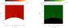 |
Fig. 7 The rotation of the plane of polarisation and relative depolarisation due to the intensity contrast and appearance of additional radiation field tensor components for two circular regions of diameter dactive region = 30 000 km and polar coordinates (θ = 6°,χ = 0°) and (θ = 6°,χ = 180°), respectively. |
By using either S1 or S2 or a combination of both, and the fact that the magnetic field is a pseudovector, one can explain all the symmetry properties of the previous graphs. These results can obviously be generalised easily to 2 or 3 dimensions, which we summarise more succinctly in the following formulae:
S1 (anterior-posterior symmetry, followed by a 180 degree rotation around the z axis)  (3)S2 (mirror reflection in the (y,z) plane)
  (4)which for S1 ⊗ S2 gives
  (5)Denoting A as the graphs resulting from dipole configuration, d, having positive components along the three axes (see Fig. 5) and B as the graphs resulting from the dipole -d (see Fig. 6), all the possibilities are contained in Table 3.2,
The outcome for all possible orientations of the dipole.
where A∗ are the graphs obtained from A by interchanging left with right and inverting the sign of the rotation angle. Similarly, B ∗ are the graphs obtained from B by performing the same operations.
Knowledge of the symmetries is very important for two reasons; i.e., on the one hand, they educate us as to what to expect when one forward-models the LOS-integrated Hanle effect of simple magnetic configurations, and on the other hand, they will prove very handy when one has to make an inversion algorithm for finding the most suitable set of parameters to fit the observations. The next important step is obviously to generalise our results to more non-symmetric dipole positions.
3.3. Polarimetry in the presence of active regions
Having shown the polarimetric outcome of a number of different magnetic dipole configurations, in order to complete the analysis of the effects of active regions, we now turn our attention to their other aspect, i.e. the symmetry breaking effect that they introduce into the radiation field anisotropy.
A very simplified picture of the underlying physics is that magnetic fields originate in the Sun’s interior, creating the loops seen in the outer atmosphere. The effect on the solar photospheric plasma is to inhibit convective motions and thus also the transport of energy to parts of the surface where the field lines are particularly dense, leading in turn to less bright areas than seen in the visible part of the electromagnetic spectrum. In the UV, however, there is an increase in the intensity contrast, which in the Lα case is ~3.4, (Raymond et al. 1997). The resulting symmetry-breaking of the radiation field tensor has tangible consequences for polarimetry. Qualitatively, these consequences can be understood by imagining being in a point, P, (which, for simplicity, is in the plane of the sky) right above an active region, typically modelled as circular with a diameter of ~30 000 km. From this position the increase in the flux is perceived symmetrically and other than increasing the polarisation degree by a small amount, there will be no other changes. But, as one moves in the horizontal direction (parallel to the solar limb), one perceives more radiation coming from the active region than the radiation coming from the average quiet sun. This increase in the flux from the active region will rotate the linear polarisation from being parallel to the solar limb (in the absence of magnetic fields and/or non-radial outflows) to being perpendicular to the line connecting the scattering atom to the centre of the active region. Diametrically opposite to this imagined position, the exact same thing will happen, but the sense of rotation will be in the opposite direction, which, for the above-mentioned parameters, is shown for two active regions whose centres have polar coordinates in degrees (θ = 6°,χ = 0°) and (θ = 6°,χ = 180°), respectively. These angles are measured in the system having z as the polar axis, whereas the azimuth is taken with respect to the x axis in the counterclockwise direction.
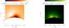 |
Fig. 8 The rotation of the plane of polarisation and relative depolarisation for the emergence of an active region onto the solar surface simulated by placing a magnetic dipole in r = (0,0,0.9) in units of solar radii, with a magnetic moment of m = (0,0.5,0), and two circular regions of diameter dactive region = 15 000 km., characterised by an intensity contrast, ΔIν. |
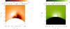 |
Fig. 9 Polarimetry of the TRACE image. |
A comparison between Fig. 7 of the present paper and Fig. 4 of Paper I, shows that the results are qualitatively identical, but that the rotation angles are much greater. This apparently inconsistent result stems from the much higher resolution of the graphs’ grid points used in these simulations, which have the effect of probing distances much closer to the sunspot centres, thus provoking much greater rotation angles and depolarisations. It must be remembered, however, that one needs a minimum amount of linear polarisation (roughly 5%) to detect the rotation angles and depolarisations and that the results with this criterion are in line with those presented in Paper I; that is, the angles one obtains at distances at which the minimum polarisation is roughly 5% are almost exactly the same and amount to ~0.1 degrees.
This very simplified view of the polarimetric effects of active regions obviously glosses over much of their varied nature and complex physical reality. When probing points as close to the active regions as we do in these simulations, some of our approximations of sects. 2.1 and 2.4 of Paper I break down. We assumed the chromospheric Lα radiation field to be independent of the heliocentric angle, with no limb-brightening or limb-darkening effects, and these approximations lose their validity the closer we approach the active regions. The additional radiation field tensor components, given in Eqs. (10) − (13) of that same paper, must also be modified in that we have to integrate over the whole solid angle as seen from the scattering point. This is, however, a somewhat academic problem in simulations of active regions, given that the overpowering effect of the relatively intense magnetic fields completely masks the modifications of the anisotropy of the radiation field.
In the general case and especially in the absence of strong magnetic fields, a more thorough way of handling the polarimetric effects of anisotropies of the radiation field tensor could be by using Carrington maps as suggested by Auchère (2005).
3.4. The full picture, dipoles and active regions
The full picture of active regions is finally achieved by combining the effects of magnetic configurations due to dipoles with those due to active regions. Their combined result is shown in Fig. 8 for a magnetic dipole in r = (0,0,0.9) in units of solar radii, with a magnetic moment of m = (0,0.5,0), two circular regions of diameter dactive region = 15 000 km., and coordinates (θ = 6°,χ = 0°,180°), characterised by an intensity contrast, ΔIν. In the starting phase of the emergence of the active region, the polarimetric signature is almost exactly the same as shown in Fig. 7 due to the overpowering effect of the intensity contrast relative to the magnetic field (m = (0,0.1,0) and dactive region = 3000 km), whereas the one caused by the end-phase (m = (0,1,0) and dactive region = 30 000 km) is almost identical to the simulation in which we have placed a magnetic dipole along the y axis (see upper right images of Figs. 3 and 4, respectively) in this case due to the overpowering effect of the magnetic field.
The tentative picture that emerges from this analysis is that, although active regions do have a measurable polarimetric effect, their ability to alter polarisation signals seems to be negligible when the magnetic field is intense, and thus can be ignored. In cases of doubt, one can, however, use their oxymoronic “visible darkness” to locate them if they are on the solar disc and subtract their contribution, and thus make a more educated guess as to the morphology and intensity of the magnetic field giving rise to the observations.
Inspired by the image made by TRACE (Fig. 2) we have tried to qualitatively simulate the magnetic scenario displayed in it by means of a combination of three dipoles and corresponding pairs of active regions. The results are shown in Fig. 9.
Needless to say, without any additional information, it would be practically impossible to infer the magnetic field morphology behind such an observation. But, luckily, this is not the case. If the physics of our simulations is correct (i.e., if active regions can be thought of as a series of magnetic dipoles and their associated active regions), then, with the aid of the combined information contained in images, such as the one made by TRACE and photospheric observations, it should be possible to hypothesise the magnetic phenomenology behind the observations by forward modelling as we have shown in this paper.
4. Conclusions
Forward modelling is an extremely useful tool in computational physics. Given certain observations containing the four Stokes parameters, one can in principle reconstruct the observed data with a modest amount of additional information by hypothesising the magnetic field configuration and by forward modelling the polarimetric outcome, thus obtaining clues to the magnetic field behind the observations.
In a previous paper we showed the effects of open polar field lines, non-radial outflows, and anisotropies in the radiation field using a self-consistent MHD model of the solar minimum corona, and have thus disclosed the effects of these polarimetrically active agents. In this paper, inspired by the beautiful images brought to us by TRACE, we concentrated on the polarimetric consequences that can be expected from the active Sun.
Through the analysis of two kinds of graphs, the rotation of the plane of polarisation with respect to the field-free case and the relative depolarisation, we show what linear polarisation parameters to expect from magnetic configurations that originate in simple magnetic dipoles and produce field intensities similar to those found in active regions. Using symmetry operations, we show that the outcome is highly degenerate, both in the Dα and RD graphs, thus warranting further information in order to distinguish between different possible configurations. We discuss, both quantitatively and qualitatively, the combined effect of magnetic fields and active regions on the solar surface, and conclude that the overpowering effect of the rather intense magnetic fields renders the radiation field effects negligible, especially at the heights (1.1 solar radii) where we propose to do the observations.
Our simulations are interesting in that they cast some more light on the dauntingly complex way of operating of the Hanle effect in LOS-integrated observations, even for simple magnetic dipole fields and a spherically symmetric corona. It is clear that much more modelling and theoretical work still needs to be done to be able to discern the correct, or most plausible, magnetic field configuration along the LOS, giving rise to some particular observation of a given portion of the plane of the sky. It would indeed be very interesting to find out how the magnetic field falls off with distance above an active region. It is quite possible that our magnetic dipole ansatz is an inadequate representation. But if this were the case, then it would also be an interesting result, because it would mean that a more sophisticated behaviour is at work, thus spurring theorists to invent more ingenious and insightful ways of modelling it. We must also as soon as observations become available, revealing hitherto unknown facts about the solar atmosphere, update our simulations by incorporating them into the code, thus diversifying parameter space and augmenting our chances of succeeding in forward modelling the magnetic phenomena of the solar corona.
It must not be forgotten, however, that the Hanle effect is complementary to the Zeeman effect and that great advantages could be obtained by performing polarimetric observations in two or more spectral lines simultaneously (Bommier et al. 1981, 1994). Moreover, tracers of the field, such as the images brought to us by TRACE, SOHO, STEREO, etc., are very valuable qualitative guides for modelling the complex physical reality of the solar corona. This possibility has already been taken into account by the groups who propose the instruments on-board future possible space missions, like SolmeX (Peter et al. 2011). If financed, it will carry a coronagraphic
UV spectropolarimeter for the first three lines of the Lyman series (the 1215.16 Å Lα, 1025 Å Lβ, and 972 Å Lγ lines) and for the 1032 Å O vi line4.
Our Sun is the best physics laboratory for understanding the origin and evolution of stellar magnetism and its interaction with the surrounding plasma. Only through a detailed understanding of this highly complex interaction will we be able to shed some light on open problems, such as coronal heating, solar wind acceleration, generation of flares, and CMEs. A knowledge of the magnetic field topology and intensity would be a tremendously important step ahead for solar physics research in that it would help theorist to make more educated guesses and select between the plethora of competing theories on all the aforementioned problems.
To this date, there are no observations available of the linear polarisation parameters in the Lα line of the solar atmosphere. Given the likelihood of succeeding in inferring the solar magnetic field by comparing forward modelling results of the Hanle effect to polarimetric observations in the Lα line, we sincerely hope that space mission proposals such as SolmeX will be financed in the not too distant future in order to make this brilliant method that has been devised and refined by many of the outstanding pioneers of solar physics flourish.
This is the estimated distance at which polarimetry becomes feasible because one needs a minimum of detectable linear polarisation in order to do measurements.
In the absence of any of the aforementioned symmetry-breaking agents, the polarisation angle is always parallel to the nearest solar limb, i.e. .
For a highly entertaining introduction to the subject of pseudovectors, the interested reader is referred to the Feynman Lectures on Physics (1963), or for a more brief introduction, Classical Electrodynamics, Jackson (1999).
Other instruments planned on SolmeX are a visible light and IR coronagraph for the 10747 Å Fe xiii line and lines in the visible part of the spectrum around 4000 Å, an EUV imaging polarimeter for the 1740 Å Fe x line, a scanning UV spectropolarimeter for lines in the 1200 − 1500 Å range, and a chromospheric magnetism explorer for the 2790 Å Mg ii and 5250 Å Fe i lines.
References
- Auchère, F. 2005, ApJ, 622, 737 [NASA ADS] [CrossRef] [Google Scholar]
- Bommier, V., & Sahal-Bréchot, S. 1982, Sol. Phys., 78, 157 [NASA ADS] [CrossRef] [Google Scholar]
- Bommier, V., Leroy, J. L., & Sahal-Bréchot, S. 1981, A&A, 100, 231 [NASA ADS] [Google Scholar]
- Bommier, V., Landi Degl’Innocenti, E., Leroy, J. L., & Sahal-Bréchot, S. 1994, Sol. Phys., 154, 231 [NASA ADS] [CrossRef] [Google Scholar]
- Derouich, M., Auchère, F., Vial, J. C., & Zhang, M. 2010, A&A, 511, A7 [NASA ADS] [CrossRef] [EDP Sciences] [Google Scholar]
- Feynman, R. P., Leighton, R. B., & Sands, M. 1963, Feynman Lectures on Physics, Chap. 52 (Addison-Wesley) [Google Scholar]
- Fineschi, S., Hoover, R. B., Fontenla, J. M., & Walker, A. B. C. 1991, Opt. Eng., 30, 1161 [NASA ADS] [CrossRef] [Google Scholar]
- Fineschi, S., Hoover, R. B., & Walker, A. B. C. 1992, SPIE, 1546, 402 [NASA ADS] [CrossRef] [Google Scholar]
- Fineschi, S., Hoover, R.B., Zukic, M., et al. 1993, SPIE, 1742, 423 [NASA ADS] [CrossRef] [Google Scholar]
- Fineschi, S., van Ballegoijen, A., & Kohl, J. L. 1999, ESA SP, 446, 317 [NASA ADS] [Google Scholar]
- Gabriel, A. H., Garton, W. R. S., Goldberg, L., et al. 1971, ApJ, 169, 595 [NASA ADS] [CrossRef] [Google Scholar]
- Hanle, W. 1924, Z. Phys., 30, 93 [Google Scholar]
- Harvey, J. W. 1969, Ph.D. Thesis, University of Colorado [Google Scholar]
- House, L. L. 1977, ApJ, 214, 236 [Google Scholar]
- House, L. L., & Smartt, R. N. 1979, in Physics of Solar Prominences, ed. E. Jensen, P. Maltby, & F. Q. Orrall, IAU Colloq., 44, 81 [Google Scholar]
- Jackson, J. D. 1999, Classical Electrodynamics (Wiley) [Google Scholar]
- Judge, P. G., Low, B. C., & Casini, R. 2006, ApJ, 651, 1229 [NASA ADS] [CrossRef] [Google Scholar]
- Khan, A., Belluzzi, L., Landi Degl’Innocenti, E., Fineschi, S., & Romoli, M. 2011, A&A, 529, A12 [NASA ADS] [CrossRef] [EDP Sciences] [Google Scholar]
- Landi Degl’Innocenti, E., & Landolfi M. 2004, Polarization in Spectral Lines (Dordrecht: Kluwer) (LL04) [Google Scholar]
- Lin, H., Penn, M. J., & Tomczyk, S. 2000, ApJ, 541, L83 [NASA ADS] [CrossRef] [Google Scholar]
- Lin, H., Kuhn, J. R., & Coulter, R. 2004, ApJ, 613, L177 [NASA ADS] [CrossRef] [Google Scholar]
- Mickey, D. L. 1973, ApJ, 181, 19 [NASA ADS] [CrossRef] [Google Scholar]
- Öhman, Y. 1929, MNRAS, 89, 479 [NASA ADS] [Google Scholar]
- Peter, H., et al. 2011, Exp. Astron., submitted [Google Scholar]
- Querfeld, C. W. 1977, Proc. SPIE, 112, 200 [NASA ADS] [Google Scholar]
- Raouafi, N. E., & Solanki, S. K. 2003, A&A, 412, 271 [NASA ADS] [CrossRef] [EDP Sciences] [Google Scholar]
- Raouafi, N. E., Solanki, S. K., & Wiegelmann, T. 2009, in Solar Polarization 5, ed. S. V. Berdyugina, K. N. Nagendra, & R. Ramelli, ASP Conf. Ser., 405, 429 [Google Scholar]
- Raymond, J. C., Kohl, J. L., Noci, G., et al. 1997, Sol. Phys., 175, 645 [NASA ADS] [CrossRef] [Google Scholar]
All Tables
All Figures
|
Fig. 1 The solar coronal thermodynamic model. |
| In the text | |
|
Fig. 2 Coronal loops as observed by TRACE in the 17.1 Å Fe ix line. Image credit: TRACE, http://apod.nasa.gov/apod/ap000928.html |
| In the text | |
|
Fig. 3 Rotation of the plane of linear polarisation with respect to the field-free case for simulations in which a magnetic dipole has been placed in r = (0,0,0.9) in units of solar radii, with a magnetic moment of m = (1,0,0), upper left, m = (0,1,0), upper right, m = (0, − 1,0), lower left, and m = (0,0,1), lower right, respectively. |
| In the text | |
|
Fig. 4 Relative depolarisations for the simulations of magnetic dipoles along the coordinate axes corresponding to Fig. 3. |
| In the text | |
|
Fig. 5 The rotation angle and relative depolarisation for |
| In the text | |
|
Fig. 6 The rotation angle and relative depolarisation for |
| In the text | |
|
Fig. 7 The rotation of the plane of polarisation and relative depolarisation due to the intensity contrast and appearance of additional radiation field tensor components for two circular regions of diameter dactive region = 30 000 km and polar coordinates (θ = 6°,χ = 0°) and (θ = 6°,χ = 180°), respectively. |
| In the text | |
|
Fig. 8 The rotation of the plane of polarisation and relative depolarisation for the emergence of an active region onto the solar surface simulated by placing a magnetic dipole in r = (0,0,0.9) in units of solar radii, with a magnetic moment of m = (0,0.5,0), and two circular regions of diameter dactive region = 15 000 km., characterised by an intensity contrast, ΔIν. |
| In the text | |
|
Fig. 9 Polarimetry of the TRACE image. |
| In the text | |
Current usage metrics show cumulative count of Article Views (full-text article views including HTML views, PDF and ePub downloads, according to the available data) and Abstracts Views on Vision4Press platform.
Data correspond to usage on the plateform after 2015. The current usage metrics is available 48-96 hours after online publication and is updated daily on week days.
Initial download of the metrics may take a while.