| Issue |
A&A
Volume 532, August 2011
|
|
|---|---|---|
| Article Number | A44 | |
| Number of page(s) | 15 | |
| Section | Planets and planetary systems | |
| DOI | https://doi.org/10.1051/0004-6361/201015873 | |
| Published online | 20 July 2011 | |
The long-term dynamics of the Jovian irregular satellites⋆
1
FUNDP, University of NamurDepartment of Mathematics and NAmur Center for Complex SYStems (NAXYS), Rempart de la Vierge 8, 5000 Namur, Belgium
e-mail: julien.frouard@fundp.ac.be
2
Institut de Mécanique Céleste et de Calcul des Éphémerides (IMCCE), Paris Observatory, UPMC, USTL, CNRS UMR 8028, Avenue Denfert-Rochereau, 75014 Paris, France
3
University of Lille 1, LAL-IMCCE, CNRS UMR 8028, 59000 Lille, France
e-mail: Alain.Vienne@univ-lille1.fr; Marc.Fouchard@univ-lille1.fr
Received: 5 October 2010
Accepted: 29 March 2011
Context. The dynamical region of the Jovian irregular satellites presents an interesting web of resonances that are not yet fully understood. Of particular interest is the influence of the resonances on the stochasticity of the individual orbits of the satellites, as well as on the long-term chaotic diffusion of the different families of satellites.
Aims. We make a systematic numerical study of the satellite region to determine the important resonances for the dynamics, to search for the chaotic zones, and to determine their influences on the dynamics of the satellites. We also compare these numerical results to previous analytical works.
Methods. Using extensive numerical integrations of the satellites along with an indicator of chaos (MEGNO), we show global and detailed views of the retrograde and prograde regions for various dynamical models of increasing complexity and indicate the appearance of the different types of resonances and the implied chaos.
Results. Along with secular and mean motion resonances that shape the dynamical regions of the satellites, we report a number of resonances involving the Great Inequality, and which are present in the system thanks to the wide range of the values of frequencies of the pericenter available for the satellites. The chaotic diffusion of the satellites is also studied and shows the long-term stability of the Ananke and Carme families, in contrast to the Pasiphae family.
Key words: planets and satellites: dynamical evolution and stability / celestial mechanics
Tables 1 and 2 are available in electronic form at http://www.aanda.org
© ESO, 2011
1. Introduction
The irregular satellites of the giant planets are one of the most peculiar populations of small bodies discovered in the Solar System. These objects are characterized by their typically high semi-major axis ratio ( ) where a⊙ is the semi-major axis of the Sun1, which can, for example, reach
  for the outermost Jovian satellite (
 for the Moon), and their highly eccentric and highly inclined orbits (respectively in the ranges [0.1–0.44] and [16°–53°]). Because they are highly perturbed by the Sun in first approximation, the satellites thus present large oscillations of their orbital elements. One direct consequence of this strong perturbation is that the classical separation between “fast” and “slow” angles, where the corresponding frequencies of the mean motion and the precessions are often separated by several orders of magnitude, does not hold here. Indeed, for the irregular satellites the typical periods of precession of the secular angles are usually not longer that 50 times their period of revolution, except for the particular cases of satellites in some secular resonances.
This particularity has been the main problem in any application of analytical methods. Indeed, the classical perturbation method, which consists in using first-order averaging over the mean anomalies of the satellites and the Sun (e.g. the suppression of the terms containing the mean anomalies in the development of the solar disturbing function), although reliable and powerful for other classes of objects, generally fails here. The problem comes from the fact that a simple averaging over the mean anomaly of the Sun suppresses important terms in the disturbing function, in particular the evection one, which has a strong effect on the frequency of the pericenter of the satellites.
Today, several works have coped with this problem by developing and using higher order perturbation methods (see Beaugé et al. 2006; Ćuk & Burns 2004). Special care has been taken in the study of (i) the secular resonance  (Saha & Tremaine 1993; Whipple & Shelus 1993; Beaugé & Nesvorný 2007; Nesvorný et al. 2003; Yokoyama et al. 2003; Ćuk & Burns 2004; Correa Otto et al. 2009), which is one of the most important secular resonances acting on the satellites; (ii) the Lidov-Kozaï resonance for distant satellites (Beaugé et al. 2006; Beaugé & Nesvorný 2007; Carruba et al. 2002; Ćuk & Burns 2004; Nesvorný et al. 2003); and (iii) the evection resonance
  (Yokoyama et al. 2008; Frouard et al. 2010; Nesvorný et al. 2003). In most of these works, the important need for the development of high-order perturbation methods or numerical ones is clearly stressed.
Concerning the dynamical studies of the Jovian satellites, an important step has been taken in the early nineties with the work of Saha & Tremaine (1993), where the authors used semi-analytical and numerical tools to investigate the dynamics of the satellites. In particular they computed the Maximal Lyapunov Exponent from the numerical integrations of Pasiphae, Sinope, Himalia, and Leda over two million years. Their results showed a possible presence of chaos, mainly for Sinope, probably originated from the overlapping of the secular resonance ν⊙ and the mean motion resonance (MMR) 6:1 with the Sun. Later works have shown that at least the totality of the satellites known in 2003 with a precisely determined orbit (30 objects) do not escape over a very long time (Nesvorný et al. 2003; see also Yokoyama et al. 2003), and averaged elements were found for these satellites that show their organization in families (Nesvorný et al. 2003, 2004), an important fact that was confirmed analytically (Beaugé & Nesvorný 2007). Concerning stability studies of the phase space structure of the satellite region, numerical integrations of fictitious satellites (Carruba et al. 2002; Yokoyama et al. 2003; Nesvorný et al. 2003; Hinse et al. 2010) confirm the different dynamical portraits obtained between prograde and retrograde regions (Hénon 1969, 1970). The study of the overall dynamical structure of the Jovian satellite region with the determination of the various important mean motion resonances for the three-body problem has been done by Hinse et al. (2010).
The aim of this paper is to investigate the long-term stability of the Jovian irregular satellites in a numerical way. We used long-term numerical integrations with a model taking the perturbations of the giant planets on the motion of the satellite into account, along with a chaos indicator, to precisely investigate the chaoticity of all the satellites, extending the works of Saha & Tremaine (1993), Beaugé & Nesvorný (2007), Nesvorný et al. (2003) and Hinse et al. (2010). The chaotic diffusion of the satellites is shown, as well as the reasons for their chaotic behavior. Stability maps of different dynamical models were computed in order to precisely show the locations and influences of the important resonances for the dynamics of the satellites. Another interest of this paper is the numerical confirmation of earlier analytical results found by previous authors.
This paper is organized as follows. In the next section we present the results of our numerical integrations of the real satellites, while their chaotic diffusion is more precisely described in Sect. 3. In Sect. 4, stability maps of the satellite regions and families are shown. Finally, we give our conclusions and point out future interesting work in Sect. 5.
2. Long-term integrations of the Jovian irregular satellites
We numerically integrate the motion of the known satellites (considered as massless particles) by using a symplectic integrator of type SBAB4 (Laskar & Robutel 2001). The Hamiltonian of the satellite is integrated in the jovicentric frame and its orbit is perturbed by the Sun and the giant planets, which are integrated using a Hamiltonian expressed in Poincaré variables (Laskar & Robutel 1995; Goździewski et al. 2008).
To check the chaoticity of the orbits, we also use a numerical indicator of chaos. There are a variety of methods that are used to determine the level of stochasticity of a given orbit and which are either based on the Lyapunov Exponents theory (see a review in Skokos 2010) such as the FLI (Froeschlé et al. 1997), the OFLI (Fouchard et al. 2002), the MEGNO (Cincotta et al. 2003), or the GALI (Skokos et al. 2007), or they are based on spectral methods, such as the frequency analysis (Laskar 2005), the spectral number (Ferraz-Mello et al. 2005), or the 0–1 test (Gottwald & Melbourne 2009). Using the frequency analysis, a two-dimensional view in the frequency space of the web of resonances of a mapping has been realized for the first time by Laskar (1993). Detailed views of the Hamiltonian case in the action space using the FLI indicator have been made by Froeschlé et al. (2000), which led to the first numerical evidence of the so-called Arnold diffusion (Lega et al. 2003).
We use the MEGNO indicator, which has been tested and used in the case of the Jovian irregular satellites by Hinse et al. (2010). We computed the MEGNO along the lines of Goździewski et al. (2008). The chaos indicators based on the Lyapunov Exponents theory are computed by using the information contained in the time evolution of one or several tangent vectors. The unique tangent vector used to determine the MEGNO is computed along with the equations of motion, by numerically integrating the variational equations (see a comprehensive recipe in Mikkola & Innanen 1999). The choice of the initial tangent vector δx0 is a recurring problem for chaos indicators based on the tangent vector method, so following Barrio et al. (2009), we choose the initial vector as the normalized gradient of the Hamiltonian H defining the motion of the satellite δx0 = ∇H/ ∥ ∇H ∥ .
An online least square fit is then applied to the MEGNO evolution for the last 85% of the numerical integration to give an indication of the Maximal Lyapunov Exponent (MLE). If such a fit is not used, we recall that in first approximation and when considering very linear MEGNO evolutions, the MLE can be directly deduced from the MEGNO value at the end of the integration by the relation  where T is the integration time. The estimation of the MLE for different satellites computed with this relation is shown in Fig. 1.
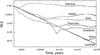 |
Fig. 1 Estimations of the MLE of seven satellites obtained from their MEGNO evolutions, in function of the integration time. |
The initial positions of the bodies were obtained from the JPL ephemerid service for the date January 1, 2008 00:00:00.00 (CT) (Julian date: 2454466.5). We made a barycentric correction of the position of the giant planets in order to add the masses of the inner planets into that of the Sun, and we used two different timesteps for the integrations, 0.01 year for prograde orbits, and 0.04 year for retrograde ones (see Nesvorný et al. 2003). The maximum relative differences of the Hamiltonians during the integrations stayed under 10-8 for the orbit of the satellite and 10-9 for the planets. We finally integrated the motion of the satellites over 100 million years. The averaged orbital elements of each satellite over the whole timespan were also computed. As a check concerning the reliability of our integrations, they can be compared with the ones found by Nesvorný et al. (2003) and show very similar values.
Table 1 shows the final MEGNO value along with an estimation of the Lyapunov time TL and the averaged orbital elements for each satellite. Quite surprisingly, the vast majority of the satellites are found to be chaotic and only three satellites which are the bulk of the Himalia prograde group show no signs of chaos during the timespan of the integration. One can see in Table 1 that the most chaotic objects are either parts of the Pasiphae family or do not actually belong to a well-defined family. The dynamical families already found by Nesvorný et al. (2003, 2004) and Beaugé & Nesvorný (2007) are of course recovered and we propose the membership of two additional satellites not previously studied. We did not use the Gauss equations (Nesvorný et al. 2003) in this work to determine their membership, but we hope that the proximity in averaged orbital elements of these new satellites compared to the families is convincing (Thelxinoe in the Ananke family, Herse in the Carme family). The (*) in Tables 1 and 2 refers to the satellites not previously studied by Nesvorný et al. (2003).
Saha & Tremaine (1993) determined the MLE of the satellites Ananke, Carme, Pasiphae and Sinope over 2 million years by using the so-called two-particle method (Benettin et al. 1976). In a paper discussing the precision of the two-particle method against the variational method, Tancredi et al. (2001) computed the MLE of the four satellites again but with the more precise variational method and found slightly different behaviors for their MLEs. To check the similarity of our results with that of Tancredi et al. (2001), we did the same computations with our numerical integrator, which uses the variational method. We found very similar evolutions of the MLEs, in particular, we recovered the result that, over the same limited integration period, Sinope and Pasiphae show clear signs of chaotic evolution. Carme and Ananke show a very weak, but still visible chaos in our simulations. We can observe the same behavior in Tancredi, Sánchez & Roig (2001). Even if their simulations show very linear evolutions of the MLE of Carme and Ananke, one can still observe slightly unstable behaviors at the very end of their computations (see the Fig. 8a of their paper).
As explained above, the first 15% of the MEGNO evolution are not used for computing the MLE. The aim is to get rid of the initial transient evolution of the tangent vector; however, for a few satellites, the MLE is found to be slower to converge, allowing a good fit of the linear part of the MEGNO only for the last 60 − 50% evolution. For example, this problem can be observed in the evolution of the MLE of Elara, Themisto and Helike in Fig. 1. For all the satellites concerned (Elara, Themisto, Carme, Callirhoe, Helike, and Hegemone), we made these improved estimations of the MLEs, with the effect of obtaining slightly higher values. We note the special case of Helike, whose LCE does not seem to converge for the considered timespan; the TL value given for this satellite corresponds to the last 85% of its MEGNO evolution and has to be considered with caution.
Using their analytical model, Beaugé & Nesvorný (2007) found the fundamental secular frequencies of the satellites. But as their model was built in the framework of the restricted three-body problem, it is interesting to check the values they found analytically, with a numerical model that takes the perturbations of the giant planets into account. To this end we made a second set of numerical integrations with the aim of determining the frequencies g and s of the satellites, which are related to the longitude of pericenter and the longitude of the node, respectively. We recall the definition of the longitude of pericenter ϖ of a satellite and its frequency g:  where Ω is the longitude of node, ω the argument of pericenter, and νH and νG their respective frequencies. The longitude of the node and its frequency s = νH are unchanged from their classical definitions. As we have shown that the vast majority of the satellites are chaotic, their orbits do not lie on quasi-periodic torus, hence their fundamental frequencies cannot be defined and thus we cannot expect the convergence of Fourier-based algorithms. Nevertheless, as the majority of the satellites are not heavily chaotic, and in particular for the most stable ones, we hope that a good definition of “stable” frequencies can be found. The timespan needed for the determination of the secular frequencies must not be too long to avoid chaotic diffusion effects, but has to be long enough to determine the most important frequencies of the system.
-
A timespan of 1 050 000 yearswas thus chosen, which is enough to resolve the secular frequen-cies of Jupiter, Saturn, and Uranus.
-
The initial timesteps being 0.01 year and 0.04 year, the output has to be decimated in order to have acceptable data for the frequency analysis, thus an output every eight years was chosen.
-
To avoid aliasing from high frequencies related to the mean motion of the satellite (typically from 130°/yr to 1030°/yr), we used a digital online low-pass filter based on the Kaiser Window (Kaiser & Reed 1977; Quinn et al. 1991). The specifications of the filter are listed here :
| Prograde | Retrograde | |
|
|
||
| Parameter β | 20 | |
| Parameter x0 | 0.0005 | 0.002 |
| Number of points | 24 001 | 6001 |
| Frequency pass (wpass) | 9°/yr | |
| Frequency stop (wstop) | 27.72°/yr | |
| Ripple | 8 × 10⁻⁷ | |
| Attenuation | 4 × 10⁻¹⁰ | |
The reader can refer to Quinn et al. (1991) for a complete presentation of the Kaiser Window and its parameters.
The maximum frequency of interest for the retrograde satellites being approximately 6°/yr, we chose a higher frequency pass to avoid any influence by the filter on the frequencies of interest. The new sampling frequency given by the eight year output being ws = 45°/yr, it satisfies the condition ws ≥ wstop + wpass to avoid aliasing in the frequencies below the frequency pass wpass (Carpino et al. 1987). An example of using the filter for the eccentricity of the retrograde satellite Pasithee is shown in Fig. 2.
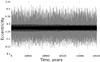 |
Fig. 2 Evolution of the osculating eccentricity of Pasithee over 50 000 years. Also shown is the corresponding online filtered eccentricity obtained using the Kaiser Window. |
The frequency analysis FMFT algorithm (Šidlichovský & Nesvorný 1996) based on the frequency analysis algorithm (Laskar 2005) is then applied to the time series of the equinoctal elements k + ih and q + ip defined by 
The secular frequencies and periods of the satellites are listed in Table 2. Not surprisingly, the secular frequencies of the satellites in each of the Ananke and Carme families are quite the same.
Concerning the Lidov-Kozaï resonance, while most of the satellites appear to be perturbed by the resonance but in a circulation mode, we found the libration of prograde Carpo around 90° during the entire integration and the close proximity of prograde Themisto to the resonance found by previous authors (Beaugé & Nesvorný 2007). The satellite Euporie appears to be in the Lidov-Kozaï resonance for the entire integration (Nesvorný et al. 2003; Ćuk & Burns 2004), its argument of pericenter ω librating around 90°. Although its motion is chaotic, it shows a very limited chaotic diffusion (see next section Fig. 5), and ω has a constant maximum deviation of ± 30° around its libration value during the timespan of the integration.
The case of 2003J18 is very interesting : we found that sometimes its motion alternates between circulation and libration in the resonance, and sometimes between the two centers of libration of the resonance ( ± 90°). This is by far the most chaotic satellite of the Jovian irregulars, but its motion does not seem to have a strong chaotic diffusion in the proper elements space (see next section Fig. 5).
Concerning the ν⊙ resonance, we found the temporary librations of the already known Pasiphae (libration around ϖ − ϖ⊙ = 0) and Sinope (libration around 0). Besides these satellites, we found three satellites that experience long periods of libration around 0: Cyllene, Helike and Hegemone. The evolution of their resonant argument is shown in Fig. 3.
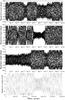 |
Fig. 3 Evolution of the resonant angle ϖ − ϖ⊙ of the satellites (from top to bottom): Cyllene, Helike, Hegemone, and 2003J02. |
These satellites have indeed long periods of precession of their pericenter as indicated in Table 2. Inspection of the periods shows that 2003J02 has an exceptionally low value of its frequency of pericenter g, and the satellite indeed switches between circulation and libration in the resonance ν⊙ around 0 (see Fig. 3).
However, we do note a bad convergence of the frequency analysis algorithm for 2003J02, which makes its values hardly reliable. In fact, this object is the farthest Jovian satellite known and is located in a very chaotic zone (see Sect. 4). We thus made two numerical integrations with 0.01 and 0.04 year timesteps to check how the timestep modifies the results. The satellite did not survive in the two integrations and shows an escape after 11.3 million years for the 0.01 year timestep and 73 million years for the 0.04 year timestep. In the two integrations the escape takes place after a rise of the satellite’s eccentricity, typical of the Lidov-Kozaï mechanism. We can hardly conclude about its macroscopic instability at this point, but do give in Table 2 the results corresponding to the 0.01 year timestep integration. Because the MEGNO evolution is very linear for this satellite, we used the simple relation shown above to obtain the MLE from the MEGNO, and we note that even if the orbital evolutions are different in the two integrations, the Lyapunov times obtained are very close to each other (1687 and 1806 years).
Among the satellites not belonging to any families, we also found several temporary librators much less affected by the resonance: Autonoe, Sponde, Orthosie and 2003J10. Their resonant arguments can be found in libration around π for periods of typically 500 000 to 106 years.
3. Chaotic diffusion of the real satellites
To study the chaotic diffusion, we use moving averaging windows in the spirit of Morbidelli & Nesvorný (1999). From the output of the 100 million year integration of a given satellite sampled every 4000 years, any orbital element x = [a,e,i] is replaced by its averaged value, 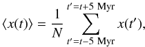 (1)where N is the number of points in each window. If the length of the windows is long enough (here we set 10 Myr), the outputs of this averaging method can be considered as numerically defined “proper” elements. Quasi-periodic orbits will present constant ⟨ x(t) ⟩ during the timespan or limited oscillations coming from non-averaged long periods, while chaotic ones will show non quasi-periodic variations. An example of this averaging method is shown in Fig. 4 for the retrograde satellite Sinope. The averaging method induces a loss of 5 Myr of the evolution at the beginning and the end of the integration.
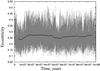 |
Fig. 4 Evolutions of the osculating and averaged eccentricity of Sinope over 100 Myr. The averaged evolution is computed using Eq. (1). |
Proceeding in the same way for all the satellites, we show the long-term evolution for the retrograde group in Fig. 5, along with ellipses indicating the known families (Nesvorný et al. 2003; Beaugé & Nesvorný 2007). From the figures, we can observe evident chaotic diffusion for the Pasiphae family and the highly-eccentric satellites lying in the range ⟨ a ⟩ = [0.155:0.165] AU. These satellites experience typical mean evolutions along the MMR 6:1 with strong oscillations in eccentricity, while their diffusion in semi-major axis are limited.
In the same spirit as in Knežević & Milani (2000) and to better differentiate the different magnitudes of diffusion, we determine for each averaged evolution the standard deviation σx and the maximum excursion Δx = ⟨ xmax ⟩ − ⟨ xmin ⟩ for the semi-major axis, eccentricity, and inclination. The results are listed in Table 1.
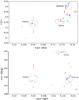 |
Fig. 5 Chaotic diffusion of the retrograde satellites over 100 Myr in semi-major axis/eccentricity (top) and semi-major axis/inclination (bottom). The colors used to distinguish the satellites are conserved between the two figures. Ellipses indicate the known retrograde families. See the online version for the color figures of the paper. |
In constrast to the Pasiphae family, the Ananke and Carme families show very limited diffusion in semi-major axis, eccentricity, and inclination. We note the interesting case of the satellite Helike at an almost constant averaged semi-major axis of 0.1398 AU, which shows on the maps (denoted by red color) important vertical diffusions in eccentricity and inclination, corresponding to an evolution in the MMR 7:1 with the Sun. For example, the argument n − 7n⊙ + s − 4g + 11s6 − 2g7 is in libration for the first 30 000 years of integration, and then alternates between libration and circulation owing to the chaoticity of the orbit. This satellite has already been found temporarily librating in the ν⊙ resonance (Fig. 3): in fact, the high-eccentricity periods of the orbit due to the MMR 7:1 put the satellite in the ν⊙ resonance, thus these high-eccentricity periods are perfectly correlated to the libration periods in the ν⊙ resonance shown in Fig. 3.
We have not shown the chaotic evolution of the satellite S2003/J2, because in our numerical integrations, as said in Sect. 2, this outermost satellite escapes before the end of the integration timespan.
Concerning the prograde satellites, there is evidence of very long periods present in their evolutions, as their averaged evolutions show characteristic quasi-periodic oscillations. For example, in the averaged evolution of Himalia, Elara, and Leda, we have found some frequencies ranging from ~1.1 million years in the semi-major axis of Himalia and Leda, up to ~33 million years in the eccentricity of Himalia.
4. Stability maps
While individual long-term integrations of the satellites give limited information on the underlying dynamics of the satellite region, much more information can be obtained from stability maps. Stability maps are commonly used to study dynamical systems, and they allow a general understanding of their resonant structure by highlighting chaotic and stable zones. Aside from their use in many other physical domains, stability maps have been used in celestial mechanics to study the dynamics of various objects like asteroids (Robutel & Laskar 2001), binary asteroids (Breiter et al. 2005), Trojans asteroids (Robutel & Gabern 2006), satellites (Callegari & Yokoyama 2010), planets of the Solar System (Michtchenko & Ferraz-Mello 2001), or extrasolar planetary systems (Érdi et al. 2004).
As we look now for the global dynamical structure acting on the satellites, we integrate a large number of fictitious orbits whose initial orbital elements were taken on regular grids of 600 × 600 orbits in semi-major axis and eccentricity or inclination. To highlight the different dynamical mechanisms, we use different dynamical models. Here, we have numerically integrated each orbit for a 100 000 year timespan for retrograde maps, and 25 000 years for prograde ones (this reduced time for prograde objects is due to computational possibilities). In each map, the initial angles of the fictitious satellites have been set to zero, except for the upper map of Fig. 6 where ϖ(0) = 90°. The numerical integration is stopped and the satellite is considered as lost if the distance of the satellite from the planet is less than the semi-major axis of the outermost Galilean satellite Callisto (taken as a = 0.0125 AU). In the same way, a satellite is considered to have been ejected if its distance exceed the Hill Sphere of Jupiter (rh = 0.355 AU) while having a positive orbital energy at the same time.
As the orbital elements of the irregular satellites typically present large oscillations, stability maps are highly dependent on the initial orbital elements chosen for the fictitious satellites. Of course, one can wait to observe the same dynamical structures (although moved and distorted) by changing the initial orbital elements. Another complication is the common difficulty of trying to indicate the positions of several real satellites on such stability maps, because real objects cannot have the same initial orbital elements. To overcome the first problem and limit the second one, we plotted the maps by using averaged orbital elements computed over the integration timespan. Moreover, this allows a better comparison with the results given by analytical models, which are usually given in terms of mean or proper variables. Frequency maps can also be used to overcome this problem (see Guzzo 2005).
In addition, the way of presenting the orbits in averaged elements allows to observe tiny secular resonances, barely noticeable when observed in initial osculating elements. This explains why the stability maps in this paper appear distorted, as with works using frequency maps, even if the free initial orbital elements are chosen on a rectangular grid.
4.1. The retrograde region
To show the different dynamical mechanisms and resonances and how they appear, we made maps for several dynamical models (Fig. 6):
-
the three-body problem (Sun + Jupiter + satellite) with the Sun ona fixed, elliptic, and inclined orbit (R3BP: Fig. 6up),
-
the three-body problem (Sun + Jupiter + satellite) with the Sun on its actual quasi-periodic orbit (R3BPQP: Fig. 6 middle);
-
the complete model used above in this paper for long-term integrations of the real satellites, which is a restricted 6 body problem: Sun + 4 giant planets + satellite (R6BP: Fig. 6 bottom).
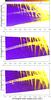 |
Fig. 6 Stability maps in semi-major axis vs eccentricity of the retrograde region for different models: R3BP (up), R3BPQP (middle), and complete model (bottom). The initial inclination is 150°. See text for comments. |
The initial inclination in all these maps has been set to 150°. All the stability maps in this paper follow the color code of the MEGNO: a value of 2 (blue) indicates stable orbits, while values over 4 (yellow) are considered to be clearly chaotic. Orbits showing a MEGNO value < 2 (black and dark blue) have a resonant behavior, while values between 2 and 4 are considered mildly chaotic for the considered timespan. The MEGNO criterion has been succesfully used for the Jovian irregular satellites system in the frame of the restricted three body problem by Hinse et al. (2010), where the authors give in particular a clear view of the position of several important MMRs, as well as general prograde and retrograde views of the outer satellite regions.
As expected, the R3BP model shows the basic dynamics and, in particular, the secular resonance ν⊙, recognizable as the large horizontal resonance across the map. This resonance will be used as a landmark in the following. In this model resonant arguments have the general form  Mean motion resonances are clearly visible as nearly vertical strips over the whole map, and, in particular, to the far right, where several MMRs are expanded into “multiplet” structures (Morbidelli 2002) corresponding to different resonant arguments in the same MMR. We can also distinguish the family of resonances n⊙ + k4s ≈ 0, as the oblique resonances.
The R3BPQP model (Fig. 6, middle) has been obtained by integrating the complete system, but without taking the direct perturbations of Saturn, Uranus, and Neptune into account on the motion of the satellite. The orbit of the Sun is thus quasi-periodic, and its frequencies can be found for example in Applegate et al. (1986), Carpino et al. (1987), or Robutel & Gabern (2006). Resonances can now be created between the frequencies of the satellites and all the frequencies of the outer Solar System contained in the spectrum of the motion of the Sun. In the R3BPQP model, the main resonances of the R3BP are conserved, although we can see that the ν⊙ resonance is considerably broader and more chaotic. This occurs because in this model the longitude of pericenter of the Sun is no longer fixed and because very slow varying arguments of type (ϖ − Φ), with Φ any of the secular angles of the giant planets, are now present in the same location (see Beaugé & Nesvorný 2007), making these resonances overlap. The main difference brought by the R3BPQP is the appearance of several secular resonances linked to the Great Inequality νGI = 2n5 − 5n6 = − 1467′′/yr between Jupiter and Saturn. These resonances have the general form  (2)where the d’Alembert rules must be assured, implying
  . In particular, a number of low-order resonances of the form
  (3)can be found across the whole map. Indeed, in the maps of Fig. 6, and following the analytical results of Ćuk & Burns (2004) and Beaugé et al. (2006), we know that for retrograde orbits the frequency g can show a large number of values depending on the orbital elements. g can be positive or negative, while the frequency s is always positive and only experiences slight variations.
The value of g is positive for orbital elements under the secular resonance ν⊙, and takes lower values while the eccentricity increases and while the orbit approaches the resonance ν⊙. All the orbits above the resonance show a frequency g < 0, with | g | increasing as the distance from ν⊙ increases. This explains why we can easily find resonances in Eq. (3) with positive and negative values of p1, using the same fixed value for p2.
In particular we can find the resonances g + νGI and 2g + νGIunder ν⊙, which have basically the same shape that ν⊙. Above ν⊙ we have found, following the previous discussion, their “symmetric” counterparts g − νGI (which is important for the Carme family) and 2g − νGI by means of numerical integrations of orbits in this area. In the following we also see that the resonance g + 2νGI is very important for the Ananke family.
Our final dynamical model is the complete one (Fig. 6 bottom). The introduction of the direct perturbations of the giant planets on the motion of the satellite basically adds more chaos to the global picture, making the resonances fuzzier than in previous models. We note that resonances of the type of Eq. (3) are in general broader, as for 2g + νGI.
4.1.1. Effect of the initial inclination
The effect of different initial inclinations for the complete model is shown on the stability map of Fig. 7, which is the complement of Fig. 6 (bottom). See also Fig. 7 (right) of Hinse et al. (2010) for the R3BP model. Along with the various vertical MMRs, the ν⊙ resonance is clearly visible as the large resonance that crosses the map almost horizontally and ends in the upper right of the map. Chaos in the bottom right of the map originates from the Lidov-Kozaï resonance (Beaugé & Nesvorný 2007) and the overlapping of MMRs.
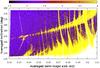 |
Fig. 7 Stability map in semi-major axis vs. inclination for the complete model. The initial eccentricity for all orbits is 0.2. |
We also computed maps similar to Fig. 6 (bottom) with different initial inclinations in Fig. 8. Each map has a different averaged inclination value. From these maps, we can state that the location of the ν⊙ resonance is in very good agreement with the analytical results of Beaugé & Nesvorný (2007) (see their Fig. 9). In particular the location of the resonance noticeably moves to higher proper eccentricity with higher inclination. The map with an initial inclination of 140° is comparatively more chaotic because of the proximity of the orbits with the Lidov-Kozaï resonance. We indicate in the maps the location and sizes of the close-up maps used to investigate the retrograde families in detail.
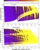 |
Fig. 8 Stability maps in semi-major axis vs. eccentricity of the retrograde region with an initial inclination of 160° (up) and 140° (bottom). The locations and sizes of the close-up maps are shown with black rectangles. |
4.1.2. Ananke, Carme and Pasiphae families
Close-up maps centered on the three retrograde families were made to study them in detail. Except for the semi-major axis and eccentricity, initial orbital elements were chosen equal to those of Ananke, Carme, and Pasiphae with the same method as in Michtchenko & Ferraz-Mello (2001) or Guzzo (2005, 2006). The diffusion in orbital elements of the members of the families is shown on the maps. We note that such a method is only “rigorous” for the study of the satellite used to compute the stability map; however, the proximity in averaged elements of the satellites belonging to a family reduces the dynamical differences and makes an unique map still usable.
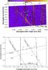 |
Fig. 9 Close-up stability map of the Ananke family along with the chaotic diffusion in orbital elements of the known satellites of the family (up). A sketch of the main dynamical features along with the averaged positions of the known satellites is also shown (bottom). |
Figure 9 is dedicated to the Ananke family area. The top panel is the stability map, while the bottom one shows the main dynamical features in the vicinity of the satellites and explained in the following. First, we observe that the members of the family are spread around the vertical 7:1 MMR with the Sun at a ~ 0.14 AU. The different vertical lines of this resonance, which lies in the range [0.139:0.141], correspond to various combinations of n − 7n⊙ with secular angles of the satellite or the planets and the long-term evolution of some of the real satellites are clearly influenced by these resonances. Of course, other MMRs are clearly seen on the map.
Several slow arguments corresponding to Eq. (2) can be found on the map. The s + 8νGI type resonance family is very important. Indeed, the striking resonance seen on the map close to the satellites corresponds to the argument s + 8νGI + 10g⊙ + 13g6, although we point out that other resonant arguments may be found at the same location. The direction of this resonance on the map indicates the general direction where the frequency of the node s is constant, thus the orbits with s = const. are located on lines parallel to this resonance. In particular, the three satellites Thelxinoe, Iocaste, and Hermippe are placed according to this direction (see Fig. 9 bottom), where the evolution of s + 8νGI is closer to zero. For example, Thelxinoe shows a very slow evolution of s + 8νGI + 23g⊙, while Iocaste is in libration in the resonance s + 8νGI + 20s7 + 3s6 for the first 60 000 years of integration (Fig. 10).
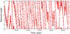 |
Fig. 10 Evolution of the angle s + 8νGI + 20s7 + 3s6 for Iocaste. |
By computing the same map as Fig. 9 along with a Fourier transform to obtain the fundamental frequencies of the fictitious orbits, we found that the argument 4g − s ≃ 0 correspond to a curve that goes through the family, although we did not found a satellite in such a resonance. Combination of the s + 8νGI and 4g − s families in this region implies that g + 2νGI ≃ 0. The remaining satellites of the family follow such a family of resonance. In particular, Fig. 11 shows the time evolution of the resonant angle g + 2νGI + g⊙ + 2g6 + 3g7 and the MEGNO for 2003J16 (gray color in Fig. 9) for 1 million years. The resonant angle librates for 400 000 years then circulates as the orbit shows
clear signs of chaotic behavior. The satellites of the Ananke family show similar evolutions.
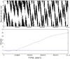 |
Fig. 11 Evolution of the satellite 2003J16. Resonant angle g + 2νGI + g⊙ + 2g6 + 3g7 (up) and MEGNO (bottom). The horizontal line in the bottom figure represents the MEGNO value for quasi-periodic orbits. |
These results can be seen from the frequency analysis of the Ananke family (Table 2), where the periods of the longitude of the pericenter Tϖ of the satellites are about half the period of the Great Inequality (883 years) and the period of precession of the node TΩ is close to  of this value.
We note the presence of chaos due to the overlapping of secular and mean motion resonances, and postulate that the chaos observed for the Ananke family arises mainly from the overlapping of the s + 8νGI secular resonance and the 7:1 MMR, while other weaker resonances of the s + 8νGI family also overlap the 7:1 MMR.
In Fig. 12 is shown the Carme family in detail. The family (except 2000J17) lies between the chaotic 6:1 MMR at a = 0.152 AU (on the left) and the 17:3 MMR at a = 0.157 AU (on the right). The mean motion resonances seem to be more chaotic in this dynamical region and we note that multiplets of mean motion resonances overlap; for example, the vertical chaotic strip which corresponds to the 17:3 MMR contains not only this resonance, but also some multiplets of the 6:1 MMR of the form n − 6n⊙ + g + 2s.
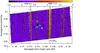 |
Fig. 12 Close-up stability map of the Carme family along with the chaotic diffusion in orbital elements of the known satellites of the family. The positions of the g − νGI and s + 10νGI secular resonances are indicated by the dotted lines. |
The secular resonance g − νGI is present on the map and draws an approximately linear curve from the bottom left to the upper right of the map, passing through the Carme family. This resonance cannot be seen in the small-sized Fig. 12, but enlargement of the figure allows this feature to be detected, thanks to the use of averaged orbital elements. Although none of the members of the family seem to be exactly in the resonance, the averaged positions of some of the satellite are very closed to it and are strongly influenced. For example, the evolution of the angle g − νGI − 3g6 − g8 + g⊙ − s8 can be found alternating from libration to circulation for Kale during the first 7 million years, but a better example is given by the evolution of the angle g − νGI − 2g6 − 2s8 for 2003J9 in Fig. 13, which shows periods of libration up to 30 million years long.
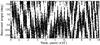 |
Fig. 13 Evolution of the resonant angle g − νGI − 2g6 − 2s8 for 2003J9. |
As for the Ananke family, this influence of the Great Inequality is confirmed by the frequency analysis of the Carme family (Table 2) where the periods of the longitude of the pericenter of the satellites are close to the period of the Great Inequality. In another way, the frequency of precession of the node s for these satellites are very close to a commensurability s + 10νGI. Indeed, we have found that the satellites of the family are strongly influenced by this resonance. They satisfy commensurabilities of the form  (4)with
  . For example, we find a 200 000 year libration of the argument s + 10νGI + l4g6 + 4g8 + 17s8 for Pasithee, and a 450 000 year libration of the angle s + 10νGI + 4g6 + 4s7 + 20s8 + s6 for Kallichore. This resonance does not appear in the stability map (Fig. 12), probably owing to the limited integration time of the map (100 000 years). Indeed, the chaotic diffusion computed for some of the real satellites of the family (100 million years) are clearly shaped in the direction of the resonance. The location of the resonance in Fig. 12 was determined by computing the frequencies of the fictitious orbits of the map.
The Pasiphae family is shown in Fig. 14. We superimposed the chaotic diffusion of the satellites of the Pasiphae family on the map, but also those of a few satellites not belonging to actual, known families: Autonoe, Eurydome, Hegemone and Sponde. We chose these satellites in such a way that their averaged inclination approximately matches that of the stability map at the same values of averaged semi-major axis and averaged eccentricity. Because the secular resonances are very sensitive to inclination and to avoid misinterpretations, we limit the number of satellites shown by allowing differences in averaged inclination of only a few degrees.
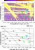 |
Fig. 14 Close-up stability map of the Pasiphae family (up) and sketch of the main resonances (bottom). The chaotic diffusion in orbital elements of the known satellites of the family and Autonoe, Eurydome, Hegemone, and Sponde is also shown. |
In contrast to the two previous retrograde families, the dynamical region of the Pasiphae family is much more chaotic, and the resonant web is clearly visible. For clarity, a separate sketch of some of the mean motion and secular resonances is also displayed with the chaotic diffusion of the satellites in Fig. 14.
The most important features are the two MMRs (6:1 and 23:4) that surround the majority of the satellites, and the secular resonance ν⊙ (S1) that again divides the map horizontally. As said above, the frequency of the longitude of pericenter g goes to zero in this location and changes its sign, thus allowing the ν⊙ resonance, and also resonances of the type  (5)where
  .
.
Many resonances can be found near the location where g ~ 0 and we find resonances involving the Great Inequality (S2) of the type  (6)where j ≥ 2 and
  , while the resonance g + νGI is indicated by S3.
As g increases when the eccentricity is decreased, resonances of the type  (7)where p ≥ 2, are present, like the g + 2νGI resonance indicated by S5. We note that we can also find the 4g + s resonance at approximately the same location, and the resonances 2g + s and 3g + s discussed in Beaugé & Nesvorný (2007) are found at lower eccentricities and thus do not appear on the stability map.
Above the ν⊙ resonance, g has a negative sign and the resonances g − νGI (S6) and g − 2νGI (S4) can be found. While these resonances overlap with the MMR 23:4 close to the pasiphae family, the chaos observed for the real satellites could only originates in the overlap of the ν⊙ resonance with resonances defined by Eqs. (5) and (6), but also with the resonance s + 11νGI (S7), which overlaps the other resonances very close to the averaged position of Pasiphae. Indeed the chaotic evolution of this satellite seems to visit the location of the ν⊙ resonance, as well as the resonances defined by Eqs. (5) and (6).
4.2. The prograde region
Figure 15 show the prograde region. In the same way as with the retrograde families, we computed the stability map using the initial orbital elements of Himalia, with semi-major axis and eccentricity taken as free parameters. As already mentioned in Hinse et al. (2010), we can see that the prograde region, which is closer to the planet than the retrograde one, is much less perturbed and dynamically “active”. Apart from the chaotic resonance located in the right of the stability map, which can be identified as the g + 8νGI + 20g⊙ + 3g6 resonance and its immediate vicinity, no chaotic orbits are found with the MEGNO indicator, which is why we restricted the MEGNO scale on the map in a tiny range of 10-3 around the stable value of 2. Indeed the MEGNO allows us to detect and distinguish resonant and unstable orbits located on border of resonances from quasi-periodic orbits (Cincotta & Simó 2000).
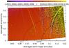 |
Fig. 15 Stability map in semi-major axis/eccentricity of the prograde region. Averaged orbital elements of the known prograde satellites are indicated by green crosses. |
The averaged positions of the six known prograde satellites are indicated on the map with crosses because their chaotic diffusion is hardly visible. The positions of Themisto and Carpo are indicated, but their averaged inclination does not match those of the stability map, which thus cannot be used to determine their stability.
Himalia, Leda, Lysithea, and Elara are located close to the g + s resonance, which can be found near the location given analytically by Beaugé & Nesvorný (2007), as well as the resonance 2g + 3s. These resonances are neither detected by the MEGNO on the stability map nor by a particular pattern that could be visible with the use of the averaged elements. Once again we show the location of these resonances on the stability map by computing the frequencies of the orbits of the map.
On the other hand, several resonances are clearly visible on the stability map. Himalia, Leda, Lysithea, and Elara in particular, are located close to a resonance satisfying g − s + 7νGI ~ 0. This resonance belongs to the family defined by 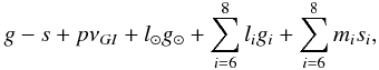 (8)where
  , and where the different possible arguments share the same shape on the stability map. Of this small prograde group, Elara is the closest to the g − s + 7νGI ~ 0 resonance, in semi-major axis, eccentricity, and inclination (we have not found an exact resonant argument satisfying Eq. (8) for this satellite) and is the only object to be detected as having a chaotic orbit. Thus we believe that the chaos of Elara comes from a possible overlapping of the g − s + 7νGI ~ 0 resonance with the g + s resonance, while longer numerical integrations would be necessary to check this hypothesis.
5. Discussion
One of the results presented above is the presence of commensurabilities involving the Great Inequality very close to or within the retrograde satellite families Ananke, Carme, and Pasiphae, as well as for the prograde group. Among these resonances, those involving the frequency of precession of the pericenter g typically have a low order.
Ćuk & Burns (2004) point out that the Great Inequality is dynamically important for the prograde irregular satellites of Saturn. In particular, they show that the fictitious satellites satisfying 2g + νGI + g6 = 0 (which implies Tϖ = 1850 years) are unstable on short timescales. This resonance induces thus a strong instability that could have had a sweeping effect on the objects captured by Saturn in the past (Ćuk & Gladman 2004). The actual Saturnian prograde satellites are not in such a resonance, but are located in inclinations above and below the resonant one.
The situation is not that clear for the Saturnian retrograde satellites, although the authors point out the case of Thrymr, which has a precession period close to that of the Great Inequality. In a general way, by checking the precession values of the irregular satellites of Saturn, Uranus, and Neptune found analytically by Beaugé & Nesvorný (2007), it seems that no important clusterings of satellites occur near commensurabilities involving the Great Inequality, except maybe a group of eight Saturnian satellites including Suttungr and Mundilfari near a 4g − 3νGI commensurability.
On the other hand, some individual satellites are very close to some resonances like Saturn’s 2004S7 (s + 3νGI) and Bergelmir (s + 2νGI), Uranus’ Ferdinand (3g − νGI), or Neptune’s Psamathe (s + νGI). One can see that commensurabilities of type s + pνGI for the satellites of Saturn, Uranus, and Neptune tend to have a lower order than in the case of Jupiter, where the satellites have higher values of s. While numerical simulations are needed, there are thus no a priori reasons to find a smaller importance of the Great Inequality in the dynamical evolution of the retrograde satellites of Saturn, Uranus and Neptune, or even with the so-called “Lesser Inequality” n7 − 2n8 between Uranus and Neptune, for the satellites of these planets.
There is confidence that the irregular satellites of the giant planets were captured during the planetary migration period caused by the gravitational scattering due to the primordial planetesimal disk (Nesvorný et al. 2007; Bottke et al. 2010). Studying the evolution of the various resonances described in this paper during the planetary migration, as considered by the models of Tsiganis et al. (2005) or Hahn & Malhotra (1999), would require careful numerical integrations. These models show that Jupiter and Saturn have migrated inward and outward respectively. In particular, they imply that no drastic change have occurred in the frequency of precession of Jupiter g5 (the amplitude of the g5 mode also changed, see Morbidelli et al. 2009), so we can only expect a very small change in the location of the ν⊙ resonance. This is not the case for resonances involving the Great Inequality. If we use the relation giving the temporal evolution of the semi-major axis a5(t) and a6(t) of Malhotra (1995) and take Jupiter and Saturn in their 1:2 mean motion resonance as initial conditions, we can see that low-order resonances of type jg + kνGI have likely crossed all the maps of Fig. 8 during the planetary migration. Carruba et al. (2004) show that a similar mechanism occurred in the region where satellites are librating in the Lidov-Kozaï resonance. Their results indicate that a powerful sweeping of objects inside the Lidov-Kozaï resonance, and caused by secondary resonances with the Great Inequality, had been acting during the migration of Jupiter and Saturn.
For the mean motion resonances between the satellites and the Sun of type pn = (p + q)n⊙, the change in semi-major axis Δa of their nominal location during this period is given by the simple relation  (9)where Δa5 is the change in semi-major axis of Jupiter (0.2 AU), and m5 and m⊙ are the masses of Jupiter and the Sun. This gives a change of ~ 0.01 AU toward the planet for the MMRs found to be close to the families (6:1, 17:3, 23:4, 7:1).
6. Conclusion
We used long-term numerical integrations of the known Jovian irregular satellites, along with a chaos indicator, to obtain a view of their mean evolution and their chaotic diffusion in the mean orbital elements space. The results show that, while the majority of the satellites show signs of chaos, the Ananke and Carme families only show restricted chaotic diffusion. On the other hand, the Pasiphae family is strongly diffusive. We plan to investigate its evolution in greater detail in future works.
By means of stability maps, we investigated the dynamical background of the prograde and retrograde regions, as well as the families’ regions. The results show that, besides the known secular resonances already studied, resonances that involved the Great Inequality between Jupiter and Saturn are quite numerous in the retrograde region. In particular, one of the most striking things is that the Ananke and Carme families are found very close to resonances of the type jg + ks + pνGI. Whether or not these resonances were important in the past dynamical history of the irregular satellite system is interesting and should be studied.
As previous analytical results by several authors were numerically confirmed in an extensive way, we can state here that, even if the three-body problem gives very good results in defining the dynamic of the satellites and predicting precession frequency values, a better approximation is given when the Sun’s orbit is taken to be quasi-periodic. This modelization must go beyond the classical Laplace-Lagrange secular approximation, as the effect of the Great Inequality must be taken into account and its related frequency itself should be present in the system.
The methods and numerical investigations presented here can be applied straighforwardly to the similar populations of irregular satellites orbiting other giant planets. Of particular interest is the case of Saturn, where resonances involving the Great Inequality were found to be very important in the dynamics of the satellites, but also in the case of Uranus and Neptune where a reduced number of satellites is known, leading to an interest in the sizes of the stable and chaotic zones around these two planets.
Because some of the satellites seems to follow a “stable chaotic” behavior, it would be interesting to check whether their orbits fulfill the conditions for applying the Nekhoroshev theorem (Nekhoroshev 1977), in order to use its spectral formulation (Guzzo 2002; Pavlović & Knežević 2009 and references therein), and thus study their stability over longer timespans.
Online material
Results of the 100 million year integration of the satellites.
Results of the frequency analysis of the satellites.
Acknowledgments
The authors would like to thank the referee for important comments that improved the presentation of this paper. J.F. is also grateful to Tobias C. Hinse for useful discussions on the dynamics of irregular satellites.
References
- Applegate, J. H., Douglas, M. R., Gursel, Y., Sussman, G. J., & Wisdom, J. 1986, AJ, 92, 176 [NASA ADS] [CrossRef] [Google Scholar]
- Barrio, R., Borczyk, W., & Breiter, S. 2009, Chaos Solitons Fractals, 40, 1697 [NASA ADS] [CrossRef] [Google Scholar]
- Beaugé, C., & Nesvorný, D. 2007, AJ, 133, 2537 [NASA ADS] [CrossRef] [Google Scholar]
- Beaugé, C., Nesvorný, D., & Dones, L. 2006, AJ, 131, 2299 [NASA ADS] [CrossRef] [Google Scholar]
- Benettin, G., Galgani, L., & Strelcyn, J.-M. 1976, Phys. Rev. A, 14, 2338 [NASA ADS] [CrossRef] [Google Scholar]
- Bottke, W. F., Nesvorný, D., Vokrouhlický, D., & Morbidelli, A. 2010, AJ, 139, 994 [NASA ADS] [CrossRef] [Google Scholar]
- Breiter, S., Melendo, B., Bartczak, P., & Wytrzyszczak, I. 2005, A&A, 437, 753 [NASA ADS] [CrossRef] [EDP Sciences] [Google Scholar]
- Callegari Jr., N., & Yokoyama, T. 2010, Planet. Space Sci., 58, 1906 [NASA ADS] [CrossRef] [Google Scholar]
- Carpino, M., Milani, A., & Nobili, A. M. 1987, A&A, 181, 182 [NASA ADS] [Google Scholar]
- Carruba, V., Burns, J. A., Nicholson, P. D., & Gladman, B. J. 2002, Icarus, 158, 434 [NASA ADS] [CrossRef] [Google Scholar]
- Carruba, V., Nesvorný, D., Burns, J. A., Ćuk, M., & Tsiganis, K. 2004, AJ, 128, 1899 [NASA ADS] [CrossRef] [Google Scholar]
- Cincotta, P. M., & Simó, C. 2000, A&ASS, 147, 205 [NASA ADS] [CrossRef] [EDP Sciences] [Google Scholar]
- Cincotta, P. M., Giordano, C. M., & Simó, C. 2003, Phys. D, 182, 151 [NASA ADS] [CrossRef] [Google Scholar]
- Correa Otto, J., Leiva, A. M., Giuppone, C. A., & Beaugé, C. 2009, MNRAS, 403, 3, 1959 [Google Scholar]
- Ćuk, M., & Burns, J. A. 2004, AJ, 128, 2518 [NASA ADS] [CrossRef] [Google Scholar]
- Ćuk, M., & Gladman, B. J. 2006, Icarus, 183, 362 [NASA ADS] [CrossRef] [Google Scholar]
- Érdi, B., Dvorak, R., Sándor, Z., Pilat-Lohinger, E., & Funk, B. 2004, MNRAS, 351, 1043 [NASA ADS] [CrossRef] [Google Scholar]
- Ferraz-Mello, S., Michtchenko, T. A., & Beaugé, C. 2005, Lect. Notes Phys. (Berlin: Springer Verlag), 683, 219 [Google Scholar]
- Fouchard, M., Lega, E., Froeschlé, C., & Froeschlé, C. 2002, Celest. Mech. & Dyn. Astr., 83, 205 [Google Scholar]
- Froeschlé, C., Gonczi, R., & Lega, E. 1997, Planet. Space Sci., 45, 881 [NASA ADS] [CrossRef] [Google Scholar]
- Froeschlé, C., Guzzo, M., & Lega, E. 2000, Science, 289, 2108 [NASA ADS] [CrossRef] [PubMed] [Google Scholar]
- Frouard, J., Fouchard, M., & Vienne, A. 2010, A&A, 515, A54 [NASA ADS] [CrossRef] [EDP Sciences] [Google Scholar]
- Gottwald, G. A., & Melbourne, I. 2009, Nonlinearity, 22, 1367 [NASA ADS] [CrossRef] [MathSciNet] [Google Scholar]
- Goździewski, K., Breiter, S., & Borczyk, W. 2008, MNRAS, 383, 989 [NASA ADS] [CrossRef] [Google Scholar]
- Guzzo, M. 2002, Celest. Mech. & Dyn. Astr., 83, 303 [NASA ADS] [CrossRef] [Google Scholar]
- Guzzo, M. 2005, Icarus, 174, 273 [NASA ADS] [CrossRef] [Google Scholar]
- Guzzo, M. 2006, Icarus, 181, 475 [NASA ADS] [CrossRef] [Google Scholar]
- Hahn, J. M., & Malhotra, R. 1999, AJ, 117, 3041 [NASA ADS] [CrossRef] [Google Scholar]
- Hénon, M. 1969, A&A, 1, 223 [NASA ADS] [Google Scholar]
- Hénon, M. 1970, A&A, 9, 24 [NASA ADS] [Google Scholar]
- Hinse, T. C., Christou, A. A., Alvarellos, J. L. A., & Goździewski, K. 2010, MNRAS, 404, 837 [NASA ADS] [CrossRef] [Google Scholar]
- Kaiser, J. F., & Reed, W. A. 1977, Rev. Sci. Instrum., 48, 1447 [NASA ADS] [CrossRef] [Google Scholar]
- Knežević, Z., & Milani, A. 2000, Celest. Mech. & Dyn. Astr., 78, 17 [Google Scholar]
- Laskar, J. 1993, Celest. Mech. Dyn. Astron., 56, 191 [Google Scholar]
- Laskar, J. 2005, in Hamiltonian systems and Fourier analysis: new prospects for gravitational dynamics, ed. Benest et al. (Cambridge Sci. Publ.), 99 [Google Scholar]
- Laskar, J., & Robutel, P. 1995, Celest. Mech. Dyn. Astron., 62, 193 [NASA ADS] [CrossRef] [MathSciNet] [Google Scholar]
- Laskar, J., & Robutel, P. 2001, Celest. Mech. Dyn. Astron., 80, 39 [NASA ADS] [CrossRef] [Google Scholar]
- Lega, E., Guzzo, M., & Froeschlé, C. 2003, Phys. D, 182, 179 [Google Scholar]
- Malhotra, R. 1995, AJ, 110, 420 [NASA ADS] [CrossRef] [Google Scholar]
- Michtchenko, T. A., & Ferraz-Mello, S. 2001, AJ, 122, 474 [NASA ADS] [CrossRef] [Google Scholar]
- Mikkola, S., & Innanen, K. 1999, Celest. Mech. & Dyn. Astr., 74, 59 [Google Scholar]
- Morbidelli, A. 2002, Modern celestial mechanics, aspects of solar system dynamics (London: Taylor & Francis) [Google Scholar]
- Morbidelli, A., & Nesvorný, D. 1999, Icarus, 139, 295 [NASA ADS] [CrossRef] [Google Scholar]
- Morbidelli, A., Brasser, R., Tsiganis, K., Gomes, R., & Levison, H. F. 2009, A&A, 507, 1041 [NASA ADS] [CrossRef] [EDP Sciences] [Google Scholar]
- Nekhoroshev, N. N. 1977, Uspekhi. Mat. Nauk, 32, 5 [Google Scholar]
- Nesvorný, D., Alvarellos, J. L. A., Dones, L., & Levison, H. F. 2003, AJ, 126, 398 [NASA ADS] [CrossRef] [Google Scholar]
- Nesvorný, D., Vokrouhlický, D., & Morbidelli, A. 2007, AJ, 133, 1962 [NASA ADS] [CrossRef] [Google Scholar]
- Pavlović, R., & Knežević, Z. 2009, Publ. Astron. Obs. Belgrade, 86, 139 [NASA ADS] [Google Scholar]
- Quinn, T. R., Tremaine, S., & Duncan, M. 1991, AJ, 101, 2287 [NASA ADS] [CrossRef] [Google Scholar]
- Robutel, P., & Gabern, F. 2006, MNRAS, 372, 1463 [NASA ADS] [CrossRef] [Google Scholar]
- Robutel, P., & Laskar, J. 2001, Icarus, 152, 4 [NASA ADS] [CrossRef] [Google Scholar]
- Saha, P., & Tremaine, S. 1993, Icarus, 106, 549 [NASA ADS] [CrossRef] [Google Scholar]
- Šidlichovský, M., & Nesvorný, D. 1996, Celest. Mech. & Dyn. Astr., 65, 137 [Google Scholar]
- Skokos, C. 2010, Lect. Notes Phys. (Berlin: Springer Verlag), 790, 63 [NASA ADS] [CrossRef] [Google Scholar]
- Skokos, C., Bountis, T. C., & Antonopoulos, C. 2007, Phys. D, 231, 30 [CrossRef] [Google Scholar]
- Tancredi, G., Sánchez, A., & Roig, F. 2001, AJ, 121, 1171 [NASA ADS] [CrossRef] [Google Scholar]
- Tsiganis, K., Gomes, R., Morbidelli, A., & Levison, H. F. 2005, Nature, 435, 459 [NASA ADS] [CrossRef] [PubMed] [Google Scholar]
- Whipple, A. L., & Shelus, P. J. 1993, Icarus, 101, 265 [NASA ADS] [CrossRef] [Google Scholar]
- Yokoyama, T., Santos, M. T., Cardin, G., & Winter, O. C. 2003, A&A, 401, 763 [NASA ADS] [CrossRef] [EDP Sciences] [Google Scholar]
- Yokoyama, T., Vieira Neto, E., Winter, O. C., Sanchez, D. M., & de Oliveira Brasil, P. I. 2008, Math. Probl. Eng., doi: 10.1155/2008/251978 [Google Scholar]
All Tables
All Figures
|
Fig. 1 Estimations of the MLE of seven satellites obtained from their MEGNO evolutions, in function of the integration time. |
| In the text | |
|
Fig. 2 Evolution of the osculating eccentricity of Pasithee over 50 000 years. Also shown is the corresponding online filtered eccentricity obtained using the Kaiser Window. |
| In the text | |
|
Fig. 3 Evolution of the resonant angle ϖ − ϖ⊙ of the satellites (from top to bottom): Cyllene, Helike, Hegemone, and 2003J02. |
| In the text | |
|
Fig. 4 Evolutions of the osculating and averaged eccentricity of Sinope over 100 Myr. The averaged evolution is computed using Eq. (1). |
| In the text | |
|
Fig. 5 Chaotic diffusion of the retrograde satellites over 100 Myr in semi-major axis/eccentricity (top) and semi-major axis/inclination (bottom). The colors used to distinguish the satellites are conserved between the two figures. Ellipses indicate the known retrograde families. See the online version for the color figures of the paper. |
| In the text | |
|
Fig. 6 Stability maps in semi-major axis vs eccentricity of the retrograde region for different models: R3BP (up), R3BPQP (middle), and complete model (bottom). The initial inclination is 150°. See text for comments. |
| In the text | |
|
Fig. 7 Stability map in semi-major axis vs. inclination for the complete model. The initial eccentricity for all orbits is 0.2. |
| In the text | |
|
Fig. 8 Stability maps in semi-major axis vs. eccentricity of the retrograde region with an initial inclination of 160° (up) and 140° (bottom). The locations and sizes of the close-up maps are shown with black rectangles. |
| In the text | |
|
Fig. 9 Close-up stability map of the Ananke family along with the chaotic diffusion in orbital elements of the known satellites of the family (up). A sketch of the main dynamical features along with the averaged positions of the known satellites is also shown (bottom). |
| In the text | |
|
Fig. 10 Evolution of the angle s + 8νGI + 20s7 + 3s6 for Iocaste. |
| In the text | |
|
Fig. 11 Evolution of the satellite 2003J16. Resonant angle g + 2νGI + g⊙ + 2g6 + 3g7 (up) and MEGNO (bottom). The horizontal line in the bottom figure represents the MEGNO value for quasi-periodic orbits. |
| In the text | |
|
Fig. 12 Close-up stability map of the Carme family along with the chaotic diffusion in orbital elements of the known satellites of the family. The positions of the g − νGI and s + 10νGI secular resonances are indicated by the dotted lines. |
| In the text | |
|
Fig. 13 Evolution of the resonant angle g − νGI − 2g6 − 2s8 for 2003J9. |
| In the text | |
|
Fig. 14 Close-up stability map of the Pasiphae family (up) and sketch of the main resonances (bottom). The chaotic diffusion in orbital elements of the known satellites of the family and Autonoe, Eurydome, Hegemone, and Sponde is also shown. |
| In the text | |
|
Fig. 15 Stability map in semi-major axis/eccentricity of the prograde region. Averaged orbital elements of the known prograde satellites are indicated by green crosses. |
| In the text | |
Current usage metrics show cumulative count of Article Views (full-text article views including HTML views, PDF and ePub downloads, according to the available data) and Abstracts Views on Vision4Press platform.
Data correspond to usage on the plateform after 2015. The current usage metrics is available 48-96 hours after online publication and is updated daily on week days.
Initial download of the metrics may take a while.