| Issue |
A&A
Volume 531, July 2011
|
|
|---|---|---|
| Article Number | A170 | |
| Number of page(s) | 4 | |
| Section | Astrophysical processes | |
| DOI | https://doi.org/10.1051/0004-6361/201117063 | |
| Published online | 08 July 2011 | |
The role of magnetic helicity for field line diffusion and drift
1
Zentrum für Astronomie und Astrophysik, Technische Universität Berlin, Hardenbergstraße 36, 10623 Berlin, Germany
e-mail: This email address is being protected from spambots. You need JavaScript enabled to view it.
2
Institut für Geowissenschaften, Naturwissenschaftliche Fakultät III, Martin-Luther-Universität Halle, 06099 Halle, Germany
e-mail: This email address is being protected from spambots. You need JavaScript enabled to view it.
Received: 11 April 2011
Accepted: 8 June 2011
Abstract
Aims. This paper discusses the systematic drift of magnetic field lines under the influence of asymmetric turbulence where the asymmetry is caused by Alfvén wave helicity.
Methods. The basic method of investigation is numerically tracing random magnetic field lines to discuss the average displacement of field lines owing to the asymmetric turbulence.
Results. The main result is that as long as one has any non-zero degree of asymmetric turbulence, there is a systematic drift of field lines on average; an effect not seen when the turbulence is taken to be symmetric. This result implies that diffusion of field lines takes place relative to the mean drift and so alters the consequences for discussions of field line diffusion.
Key words: plasmas / magnetic fields / turbulence / waves
© ESO, 2011
1. Introduction
The structure of magnetic field lines plays an important role for charged particles such as cosmic rays or solar wind particles. Turbulent magnetic fields lead to scattering and deflection of the particles both in the interstellar and the interplanetary medium. In general, magnetic field lines are randomly fluctuating and have to be described as stochastic (Jokipii & Parker 1969). Therefore, it is necessary to use statistical quantities such as the mean square displacement, ⟨ (Δr ⊥ )2 ⟩ , where Δr ⊥ = (x − x0,y − y0) with (x0, y0) the initial position of the field line in the direction perpendicular to the background field, and angular brackets ⟨ · ⟩ denote ensemble averages.
Discussing magnetic field line random walk (FLRW) in two or three dimensions (e.g., Jokipii & Parker 1969; see also Isichenko 1992; Bakunin 2010, for an introduction) is important in the astrophysical context because field line displacement can be used as an intermediate step to investigate particle scattering (Matthaeus et al. 2003; Shalchi & Kourakis 2007b; Tautz et al. 2008) via the compound diffusion approach (e.g., Kóta & Jokipii 2000; Webb et al. 2006). For FLRW, several analytical theories have been proposed to describe the random walk of stochastic magnetic field lines (Matthaeus et al. 1995; Zimbardo et al. 2000; Ruffolo et al. 2006; Shalchi & Kourakis 2007a; Shalchi et al. 2009; Shalchi & Weinhorst 2009; Shalchi & Qin 2010). Conventionally, several approximations are made to facilitate the calculations. For example, in many analytical theories it is assumed that field line separation is a diffusive process characterized by a finite diffusion coefficient and accordingly requiring ⟨ (Δr ⊥ )2 ⟩ ∝ Δz. However, this depends sensitively on the geometry and the spectral properties assumed for the turbulence (Shalchi & Kourakis 2007a; Shalchi & Qin 2010).
Recently, Tautz & Lerche (2011) re-investigated FLRW from first principles and showed that it is not permitted to neglect the turbulent field component parallel to the background field because this can lead to a non-vanishing expectation value of the separation distance perpendicular to the symmetry axis, i.e., ⟨ Δr ⊥ ⟩ ≠ 0, which appears as an additional force acting on particles that follow these field lines. A prerequisite is non-axisymmetric turbulence (Ruffolo et al. 2006; Weinhorst et al. 2008), which can be identified with a non-vanishing magnetic helicity (e.g., Schlickeiser 1989; Dung & Schlickeiser 1990b,a).
Physically, the study of non-axisymmetric turbulence is motivated by the following examples (cf. Ruffolo et al. 2006, 2008): (i) early measurements in the solar system revealed a 4:3 ratio of solar wind fluctuation energy in the azimuthal direction relative to the radial and the z directions (Belcher & Davids 1971); (ii) the solar wind near Earth has a two-dimensional (2D) turbulence component that is symmetric with respect to the mean field, while another component has wave vectors along the radial direction. But the mean magnetic field follows a spiral structure, thus breaking the axisymmetry (Saur & Bieber 1999); (iii) non-axisymmetric fluctuations may be important in enhanced latitudinal transport of cosmic rays at high heliographic latitudes (Jokipii et al. 1995; Burger & Hattingh 1998). Theoretically, therefore, the result has far-reaching consequences for our understanding of the diffusion of these field lines as well as for particle motion in these magnetic fields, which now must diffuse relative to ⟨ Δr ⊥ ⟩ instead of with respect to the direction of the background field, B0.
In this research note, therefore, numerical test-particle simulations will be performed to investigate the effect of drifting magnetic field lines in non-axisymmetric turbulent magnetic structures. For both magnetostatic and Alfvénic turbulence, cases with and without magnetic helicity are compared to work out the field line drift effect. Because Alfvén waves are believed to contribute substantially to the observed heliospheric magnetic turbulence (Jokipii 1973), this provides a good example for a numerical study.
The paper is organized as follows: Sect. 2 describes the simulation setup and the procedure used for the numerical calculation of field line mean coordinates and field line diffusion coefficients. In Sect. 3 two different sets of simulation results are shown that underline the presence of a field line drift. Section 4 provides a short summary and a discussion of the results.
2. Simulation design
In the Padian code (Tautz 2010a), magnetic turbulence is generated through the superposition of a large number (usually 102–103) of plane waves (Giacalone & Jokipii 1999; Tautz 2010a) with random polarization and phase angles.
The turbulent magnetic field can be written in the form  (1)where N is the number of the sampling points in wavenumber space. The primed coordinates are calculated from a rotation matrix with random angles, and
  is the unit polarization vector in the x′-y′ plane. The βn are random phase angles.
For one of the simulation sets, magnetostatic turbulence is used. For the other simulation sets, propagating Alfvén waves with ω = vAk ∥ are used (Michałek 2001; Tautz 2010b), with the Alfvén speed  , where ρ is the particle density. Circular (or elliptic) and linear polarized waves are obtained by specifying the x and y components of the unit vector so that one has either a rotating or a constant direction of the magnetic field vector.
Furthermore, the turbulence power spectrum G needs to be specified, which defines the distribution of turbulence energy per wave number interval (Shalchi & Weinhorst 2009) ![Mathematical equation: \begin{equation} \label{eq:spect} G(k)\propto\frac{\left(\ell_0 k\right)^q}{\bigl[1+\left(\ell_0k\right)^2\bigr]^{(s+q)/2}}, \end{equation}](/articles/aa/full_html/2011/07/aa17063-11/aa17063-11-eq23.png) (2)where q and s are the energy range and the inertial range spectral indices, respectively. The turbulence bend-over scale, ℓ0, marks the transition between energy and inertial ranges and serves as a reference length. For q = 0 a spectrum with a constant energy range is obtained, which will be used in the present article. With s = 5 / 3, a Kolmogorov-type power law is obtained in the inertial range, i.e., for k ≫ ℓ-1.
(2)where q and s are the energy range and the inertial range spectral indices, respectively. The turbulence bend-over scale, ℓ0, marks the transition between energy and inertial ranges and serves as a reference length. For q = 0 a spectrum with a constant energy range is obtained, which will be used in the present article. With s = 5 / 3, a Kolmogorov-type power law is obtained in the inertial range, i.e., for k ≫ ℓ-1.
For each turbulence realization, i.e., each different set of random numbers for Eq. (1), the magnetic field line equation ![Mathematical equation: \begin{equation} \label{eq:Beq} \dd[\f r]s=\frac{\f B\bigl(\f r(s)\bigr)}{\abs{\f B}}=\frac{B_0\ez+\delta\f B\bigl(\f r(s)\bigr)}{\abs{\f B}}, \end{equation}](/articles/aa/full_html/2011/07/aa17063-11/aa17063-11-eq30.png) (3)is numerically integrated using either a Bulirsch-Stoer (Stoer & Bulirsch 2002) method or the Dorman-Prince 853 (Hairer et al. 1993) method, each with adaptive step size. The latter is based on the Runge-Kutta technique but has additional, embedded error estimation methods (Press et al. 2007). From Eq. (3)the three-dimensional field line r(s) is obtained, where s is a trace parameter of the space curve.
(3)is numerically integrated using either a Bulirsch-Stoer (Stoer & Bulirsch 2002) method or the Dorman-Prince 853 (Hairer et al. 1993) method, each with adaptive step size. The latter is based on the Runge-Kutta technique but has additional, embedded error estimation methods (Press et al. 2007). From Eq. (3)the three-dimensional field line r(s) is obtained, where s is a trace parameter of the space curve.
 |
Fig. 1 Turbulent field lines as obtained from the Padian simulation code for isotropic magnetostatic and axisymmetric turbulence. Shown is the projection on the z-y plane of field lines distributed along the x axis with initially z(x0) = 0. |
The mean perpendicular coordinates, ⟨ Δx ⟩ and ⟨ Δy ⟩ , are obtained by averaging over a large number of field lines with different initial positions. For the simulations shown here, typically 100 field lines are distributed over a range of 200ℓ0, each being integrated in 100 different turbulence realizations. In Fig. 1 some sample field lines are shown to illustrate that while some field lines have a large perpendicular displacement Δr ⊥ ~ Δz, the mean value ⟨ Δr ⊥ ⟩ is approximately zero. This is different for a non-vanishing magnetic helicity, i.e., a non-axisymmetric turbulence. The general effect of these turbulent structures, therefore, leads to a non-vanishing perpendicular displacement of the field lines, i.e., ⟨ Δr ⊥ ⟩ ≠ 0.
Furthermore, the (running) perpendicular field line diffusion coefficients can then be obtained by calculating  (4)Note that in contradiction to the term “diffusion” coefficient, κFL does not necessarily have a finite value in the limit of large |z| → ∞ as would be required for a diffusive process. Instead, a number of articles (Shalchi & Kourakis 2007a,c; Tautz et al. 2008; Shalchi & Qin 2010) have shown that often super- or sub-diffusion is found, i.e., (d / dz)κFL > 0 or < 0, respectively.
3. Results
In this section, results from the two different sets of numerical simulations are shown, the first of which uses isotropic magnetostatic turbulence, whereas the second operates in isotropic turbulence composed of circular or linearized Alfvén waves.
3.1. Isotropic magnetostatic turbulence
In Tautz et al. (2008) it has been shown that for the field line diffusion coefficient in isotropic turbulence the quasi-linear theory provides a good description. For the spectrum from Eq. (2)with q = 0, the perpendicular mean square displacement of the magnetic field lines can be calculated as 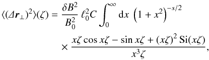 (5)where ζ = z / l0 and where Si denotes the sine integral function (Gradshteyn & Ryzhik 2000). Furthermore, C ≈ 0.11886 is a normalization constant that depends on s.
Using a Taylor expansion of the expression in the second line of Eq. (5)and the limit of large |z| ≫ ℓ0, a simplified result can be obtained, which reads ![Mathematical equation: \begin{equation} \label{eq:Dx_fl2} \langle(\De\f r\se)^2\rangle(\zeta)\simeq\frac{\delta B^2}{B_0^2}\,\ell_0^2C\,\frac{\pi\zeta}{2}\left[1+\frac{1}{s}+\ln\!\left(\frac{4\zeta}{3\pi}\right)\right]\cdot \end{equation}](/articles/aa/full_html/2011/07/aa17063-11/aa17063-11-eq48.png) (6)
(6)
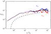 |
Fig. 2 Perpendicular field line diffusion coefficient, κFL, for isotropic magnetostatic turbulence with vanishing magnetic helicity (i.e., axisymmetric). Shown are the simulation results for the x and y directions (blue and red lines, respectively), the averaged value (black) as well as the perpendicular diffusion coefficient. The dashed and dotted lines illustrate the quasi-linear result from Eqs. (5)and (6), respectively. |
In Fig. 2 the quasi-linear perpendicular field line diffusion coefficient in isotropic turbulence from Eq. (6)is shown as a function of the distance parallel to the background magnetic field, thereby illustrating the logarithmic super-diffusion of the running perpendicular field line diffusion coefficient. Furthermore, the corresponding simulation results are also shown in Fig. 2. Bearing in mind that quasi-linear theory involves severe approximations and is valid only for large |z| ≫ ℓ0, an overall agreement between the analytical theory and the numerical result can be confirmed, although the simulations exhibit strong fluctuations. Furthermore, no qualitative difference is found for non-axisymmetry.
In Fig. 3 the x and y components together with the averaged value of the mean perpendicular coordinate are shown for the axisymmetric case as well as for two non-axisymmetric cases. The latter are obtained by confining the direction of the wave vectors in Eq. (1)to a more or less narrow angle in the x-y direction; for Fig. 3, the value range in φ ∈ [ − π / 2,π / 2 ] and φ ∈ [ − π / 8,π / 4 ] . This illustrates a clearly visible systematic drift of the magnetic field lines in different directions; this effect is not exhibited for the axisymmetric case. That one has ⟨ Δr ⊥ ⟩ = (⟨ Δx ⟩ + ⟨ Δy ⟩ ) / 2 ≈ 0 in panel (b) of Fig. 3 for the averaged perpendicular drift is a mere coincidence. Because here the turbulence is artificially confined to a cone in the x-z directions, the x drift behaves differently from the y drift.
3.2. Alfvénic turbulence
In contrast to magnetostatic isotropic turbulence, where all directions of the turbulent wave vector have equal probability, Alfvénic turbulence is centered around the direction of the background field, which is the direction of wave propagation. In that sense, the turbulence is no longer isotropic (even though it is often being called isotropic; see Michałek 2001; Schlickeiser 2002). In a sense, such a turbulence model is more comparable to the slab model, which has been used for a long time for reasons of mathematical simplification (e.g., Jokipii 1966; Shalchi et al. 2007). Superposed with its counterpart, which is the 2D model, the composite slab/2D model has been widely used in cosmic ray transport theory (see, e.g., Bieber et al. 1994). To some extent, the composite model can even be physically motivated by solar wind observations (Matthaeus et al. 1990), which confirms the existence of an elongated structure in the correlation function.
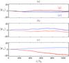 |
Fig. 3 Mean perpendicular coordinate in isotropic magnetostatic turbulence. In panel a) the axisymmetric case is shown, whereas in panels b) and c) the turbulent wave vectors are confined to a cone with the opening angle |


The advantage of the Alfvén wave model is that one can easily switch on (i) the magnetic helicity, σ, by restricting the Alfvén waves to either linear polarization waves or by using circular polarized waves with only one handedness; (ii) the cross helicity, Hc, by controlling the ratio of forward and backward moving waves.
In Fig. 4 the field line diffusion coefficient. κFL, is shown, illustrating that the behavior is changed qualitatively owing to the magnetic helicity. Without magnetic helicity, κFL is weakly subdiffusive, while diffusion is recovered for circular polarized Alfvén waves. This is different from the magnetostatic turbulence in Sect. 3.1.
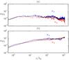 |
Fig. 4 Perpendicular field line diffusion coefficient, κFL, for isotropic Alfvénic turbulence. In panel a) linear polarized Alfvén waves with vanishing cross helicity were used; hence the turbulence is axisymmetric. In panel b) circular polarized Alfvén waves were used that are all of the same handedness so that the magnetic helicity is maximal. The colors are the same as in Fig. 2. |
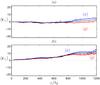 |
Fig. 5 Mean perpendicular coordinate in Alfvénic turbulence. Panels a) and b) correspond to the cases shown in Fig. 4. |
The comparison of the mean perpendicular coordinate for both cases is shown in Fig. 5, where for a non-vanishing magnetic helicity, a strong drift motion of the field lines can be observed. This agrees with the prediction of Tautz & Lerche (2011), who showed that as soon as the turbulence is no longer axisymmetric, a mean perpendicular displacement of the field lines is found.
4. Summary and conclusion
The effect of drifting magnetic field lines due to a non-vanishing magnetic helicity in turbulent magnetic fields was investigated using a numerical Monte-Carlo simulation code. As has been shown recently, the assumption δBz ≈ 0 can lead to incorrect results if the turbulence is not axisymmetric. Non-axisymmetric magnetostatic turbulence was realized by confining the wave vectors of the Fourier modes to a cone in the x-z plane with opening angles between π / 4 and π / 2, thereby breaking the symmetry around the axis of the background magnetic field. In a second simulation set, Alfvén waves were used in a second simulation set, where (i) linear polarization corresponds to axisymmetry; (ii) circular polarization with only one handedness introduces a non-zero magnetic helicity and thus breaks the axisymmetry. The results show a strong transverse drift motion of the field lines, an effect not incorporated at all when the turbulence is assumed to be axisymmetric.
The simulation results exhibit strong fluctuations so that even in axisymmetric cases, the mean perpendicular displacement, ⟨ Δr ⊥ ⟩ , is not precisely zero. However, as soon as the magnetic helicity does not vanish, a systematic deviation from zero was found in all cases1. Therefore, the results are significant, indicating that a field line drift is indeed found in non-axisymmetric turbulence. The use of turbulence that is asymmetric, which more closely mirrors reality than an assumed perfectly symmetric situation, brings to light new effects of field line drift that have to be accounted for in discussions of field line diffusion and that then alter the perception of the underlying physical behavior in these turbulent systems. Because measurements indicate that magnetic turbulence in the solar wind has indeed a non-axisymmetric component (e.g., de Koning & Bieber 2003), these results may be important for the interpretation of energetic particle events (e.g., Schlickeiser et al. 2009). Future work should, therefore, investigate the quantitative difference of the effect in relativistic solar wind turbulence (Matthaeus et al. 1990).
Note that magnetic helicity is not mirror symmetric. According to Eq. (26) in Tautz & Lerche (2011), the sign of ⟨ Δr ⊥ ⟩ is changed if the helicity is reversed, i.e., if Alfvén waves with circular polarization of opposite sign are used.
References
- Bakunin, O. G. 2010, Turbulence and Diffusion (Berlin, Heidelberg: Springer) [Google Scholar]
- Belcher, J. W., & Davids, L. 1971, J. Geophys. Res., 76, 3534 [NASA ADS] [CrossRef] [Google Scholar]
- Bieber, J. W., Matthaeus, W. H., Smith, C. W., et al. 1994, ApJ, 420, 294 [Google Scholar]
- Burger, R. A., & Hattingh, M. 1998, ApJ, 505, 244 [NASA ADS] [CrossRef] [Google Scholar]
- de Koning, C. A., & Bieber, J. W. 2003, in Proceedings of the 28th International Cosmic Ray Conference, ed. T. Kajita, Y. Asaoka, A. Kawachi, Y. Matsubara, & M. Sasaki, 3713 [Google Scholar]
- Dung, R., & Schlickeiser, R. 1990a, A&A, 240, 537 [NASA ADS] [Google Scholar]
- Dung, R., & Schlickeiser, R. 1990b, A&A, 237, 504 [NASA ADS] [Google Scholar]
- Giacalone, J., & Jokipii, J. R. 1999, ApJ, 520, 204 [Google Scholar]
- Gradshteyn, I. S., & Ryzhik, I. N. 2000, Table of Integrals, Series, and Products (London: Academic Press) [Google Scholar]
- Hairer, E., Nørsett, S. P., & Wanner, G. 1993, Solving Ordinary Differential Equations I, Nonstiff Problems, 2nd edn. (New York: Springer) [Google Scholar]
- Isichenko, M. B. 1992, Rev. Mod. Phys., 64, 961 [NASA ADS] [CrossRef] [Google Scholar]
- Jokipii, J. R. 1966, ApJ, 146, 480 [Google Scholar]
- Jokipii, J. R. 1973, ApJ, 182, 585 [NASA ADS] [CrossRef] [Google Scholar]
- Jokipii, J. R., & Parker, E. N. 1969, ApJ, 155, 777 [NASA ADS] [CrossRef] [Google Scholar]
- Jokipii, J. R., Kóta, J., Giacalone, J., Horbury, T. S., & Smith, E. J. 1995, Geophys. Res. Lett., 22, 3385 [NASA ADS] [CrossRef] [Google Scholar]
- Kóta, J., & Jokipii, J. R. 2000, ApJ, 531, 1067 [NASA ADS] [CrossRef] [Google Scholar]
- Matthaeus, W. H., Goldstein, M. L., & Aaron, R. D. 1990, J. Geophys. Res., 95, 20673 [Google Scholar]
- Matthaeus, W. H., Gray, P. C., Pontius Jr., D. H., & Bieber, J. W. 1995, Phys. Rev. Lett., 75, 2136 [Google Scholar]
- Matthaeus, W. H., Qin, G., Bieber, J. W., & Zank, G. P. 2003, ApJ, 590, L53 [Google Scholar]
- Michałek, G. 2001, A&A, 376, 667 [NASA ADS] [CrossRef] [EDP Sciences] [Google Scholar]
- Press, W. H., Teukolsky, S. A., Vetterling, W. T., & Flannery, B. P. 2007, Numerical Recipes (Cambridge: University Press) [Google Scholar]
- Ruffolo, D., Chuychai, P., & Matthaeus, W. H. 2006, ApJ, 644, 971 [NASA ADS] [CrossRef] [Google Scholar]
- Ruffolo, D., Chuychai, P., Wongpan, P., et al. 2008, ApJ, 686, 1231 [NASA ADS] [CrossRef] [Google Scholar]
- Saur, J., & Bieber, J. W. 1999, J. Geophys. Res., 104, 9975 [Google Scholar]
- Schlickeiser, R. 1989, ApJ, 336, 243 [NASA ADS] [CrossRef] [Google Scholar]
- Schlickeiser, R. 2002, Cosmic Ray Astrophysics (Berlin: Springer) [Google Scholar]
- Schlickeiser, R., Artmann, S., & Dröge, W. 2009, Open Plasma Phys. J., 2, 1 [NASA ADS] [CrossRef] [Google Scholar]
- Shalchi, A., & Kourakis, I. 2007a, Phys. Plasmas, 14, 092903 [NASA ADS] [CrossRef] [Google Scholar]
- Shalchi, A., & Kourakis, I. 2007b, A&A, 470, 405 [NASA ADS] [CrossRef] [EDP Sciences] [Google Scholar]
- Shalchi, A., & Kourakis, I. 2007c, Phys. Plasmas, 14, 112901 [NASA ADS] [CrossRef] [Google Scholar]
- Shalchi, A., & Qin, G. 2010, Astrophys. Space Sci., 330, 279 [NASA ADS] [CrossRef] [Google Scholar]
- Shalchi, A., & Weinhorst, B. 2009, Adv. Space Res., 43, 1429 [NASA ADS] [CrossRef] [Google Scholar]
- Shalchi, A., Tautz, R. C., & Schlickeiser, R. 2007, A&A, 475, 415 [NASA ADS] [CrossRef] [EDP Sciences] [Google Scholar]
- Shalchi, A., le Roux, J. A., Webb, G. M., & Zank, G. P. 2009, Phys. Rev. E, 80, 066408 [NASA ADS] [CrossRef] [Google Scholar]
- Stoer, J., & Bulirsch, R. 2002, Introduction to Numerical Analysis, 3rd edn. (New York: Springer) [Google Scholar]
- Tautz, R. C. 2010a, Computer Phys. Commun., 81, 71 [Google Scholar]
- Tautz, R. C. 2010b, Plasma Phys. Contr. Fusion, 52, 045016 [Google Scholar]
- Tautz, R. C., & Lerche, I. 2011, Phys. Lett. A, 375, 2587 [NASA ADS] [CrossRef] [Google Scholar]
- Tautz, R. C., Shalchi, A., & Schlickeiser, R. 2008, ApJ, 672, 642 [NASA ADS] [CrossRef] [Google Scholar]
- Webb, G. M., Zank, G. P., Kaghashvili, E. K., & le Roux, J. A. 2006, ApJ, 651, 211 [NASA ADS] [CrossRef] [Google Scholar]
- Weinhorst, B., Shalchi, A., & Fichtner, H. 2008, ApJ, 677, 671 [NASA ADS] [CrossRef] [Google Scholar]
- Zimbardo, G., Veltri, P., & Pommois, P. 2000, Phys. Rev. E, 61, 1940 [NASA ADS] [CrossRef] [Google Scholar]
All Figures
|
Fig. 1 Turbulent field lines as obtained from the Padian simulation code for isotropic magnetostatic and axisymmetric turbulence. Shown is the projection on the z-y plane of field lines distributed along the x axis with initially z(x0) = 0. |
| In the text | |
|
Fig. 2 Perpendicular field line diffusion coefficient, κFL, for isotropic magnetostatic turbulence with vanishing magnetic helicity (i.e., axisymmetric). Shown are the simulation results for the x and y directions (blue and red lines, respectively), the averaged value (black) as well as the perpendicular diffusion coefficient. The dashed and dotted lines illustrate the quasi-linear result from Eqs. (5)and (6), respectively. |
| In the text | |
|
Fig. 3 Mean perpendicular coordinate in isotropic magnetostatic turbulence. In panel a) the axisymmetric case is shown, whereas in panels b) and c) the turbulent wave vectors are confined to a cone with the opening angle |
| In the text | |
|
Fig. 4 Perpendicular field line diffusion coefficient, κFL, for isotropic Alfvénic turbulence. In panel a) linear polarized Alfvén waves with vanishing cross helicity were used; hence the turbulence is axisymmetric. In panel b) circular polarized Alfvén waves were used that are all of the same handedness so that the magnetic helicity is maximal. The colors are the same as in Fig. 2. |
| In the text | |
|
Fig. 5 Mean perpendicular coordinate in Alfvénic turbulence. Panels a) and b) correspond to the cases shown in Fig. 4. |
| In the text | |
Current usage metrics show cumulative count of Article Views (full-text article views including HTML views, PDF and ePub downloads, according to the available data) and Abstracts Views on Vision4Press platform.
Data correspond to usage on the plateform after 2015. The current usage metrics is available 48-96 hours after online publication and is updated daily on week days.
Initial download of the metrics may take a while.