| Issue |
A&A
Volume 531, July 2011
|
|
|---|---|---|
| Article Number | A102 | |
| Number of page(s) | 9 | |
| Section | Astronomical instrumentation | |
| DOI | https://doi.org/10.1051/0004-6361/201116918 | |
| Published online | 21 June 2011 | |
Data-reduction techniques for high-contrast imaging polarimetry
Applications to ExPo
Sterrekundig Instituut, Universiteit Utrecht PO Box 80000 3508 TA Utrecht The Netherlands
e-mail: H.CanovasCabrera@uu.nl
Received: 18 March 2011
Accepted: 10 May 2011
Context. Imaging polarimetry is a powerful tool for detecting and characterizing exoplanets and circumstellar environments. Polarimetry allows a separation of the light coming from an unpolarized source such as a star and the polarized source such as a planet or a protoplanetary disk. Future facilities like SPHERE at the VLT or EPICS at the E-ELT will incorporate imaging polarimetry to detect exoplanets. The Extreme Polarimeter (ExPo) is a dual-beam imaging polarimeter that can currently reach contrast ratios of 105, enough to characterize circumstellar environments.
Aims. We present the data-reduction steps for a dual-beam imaging polarimeter that can reach contrast ratios of 105.
Methods. The data obtained with ExPo at the William Herschel Telescope (WHT) are analyzed. Instrumental artifacts and noise sources are discussed for an unpolarized star and for a protoplanetary disk (AB Aurigae).
Results. The combination of fast modulation and dual-beam techniques allows us to minimize instrumental artifacts. A proper data processing and alignment of the images is fundamental when dealing with high contrasts. Imaging polarimetry proves to be a powerful method to resolve circumstellar environments even without a coronagraph mask or an adaptive optics system.
Key words: instrumentation: polarimeters / polarization / techniques: polarimetric / methods: data analysis / circumstellar matter
© ESO, 2011
1. Introduction
The direct detection and characterization of exoplanets is one of the main goals of the next generation of instruments and telescopes, such as the E-ELT (Hook 2009). Despite the increasing amount of detected exoplanets (e.g., http://www.exoplanet.eu/), only a few of them have been directly imaged (Marois et al. 2008; Kalas et al. 2008; Lagrange et al. 2010; Todorov et al. 2010).
Polarization is a powerful tool for detecting and characterizing circumstellar environments, such as protoplanetary disks, debris disks, and exoplanets (Kuhn et al. 2001; Stam et al. 2005, 2006). While the light coming from the star is largely unpolarized, the scattered light from exoplanets and circumstellar environments is highly (linearly) polarized. This makes it easy to separate the planet signal from the unpolarized starlight, and reach the required high contrast ratios.
Future exoplanet instruments such as SPHERE (Thalmann et al. 2008), GPI (Graham et al. 2007) or EPICS (Kasper et al. 2010) will include imaging polarimetry, spectropolarimetry, or both, to characterize exoplanets. To reach the high contrast ratios that are necessary to detect an exoplanet, these instruments will combine coronagraphs, adaptive optics, and polarimetry. The combination of the firsts two elements can reduce the stellar light by a factor of 106 (Martinez et al. 2010), while polarimetry alone can reach contrast ratios of 105 (Rodenhuis et al., in prep.). The identification of instrumental artifacts and spurious signals that appear at these extremely high ratios is fundamental for understanding the data produced by the new generation of exoplanet imagers.
ExPo is a dual-beam imaging polarimeter that combines speckle imaging with dual-beam techniques, currently reaching contrast ratios of 105 without a coronagraph or adaptive optics system (Rodenhuis et al. 2008; 2011, in prep.). The sensitivity reached by this instrument allows us to image circumstellar environments such as protoplanetary disks or dust shells with unprecedented accuracy (e.g. Canovas et al. 2011a,b, in prep.)
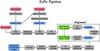 |
Fig. 1 Pipeline Block Diagram. |
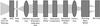 |
Fig. 2 Schematic layout of the instrument in the Nasmyth focus of a telescope. |
In this paper we present the data-reduction approach for high dynamic range polarimetry. The whole data-reduction process is shown in Fig. 1. Results show that the dual-beam technique effectively minimizes systematic errors, leading to sensitive polarization measurements of different circumstellar environments.
In the following sections, the instrument is briefly described, followed by the analysis of the instrumental artifacts. The image-reduction process and a discussion of first results are presented at the end. Preliminary results of the well-known protoplanetary disk AB Aurigae and the diskless star HD 12815 are shown.
2. Instrument description
ExPo is a dual-beam imaging polarimeter that currently reaches contrast ratios of 105. It is designed to characterize circumstellar environments, such as the disks around Herbig Ae/Be and T Tauri stars. ExPo is currently a visitor instrument at the William Herschel Telescope (WHT), where it has been used for four successful observing campaigns.
ExPo has a wavelength range from 400 − 900 nm, and its field of view is 20′′ × 20′′. It works with exposure times of 0.028 seconds to minimize the effects of atmospheric seeing. Systematic errors are minimized by modulating two opposite polarization states. The combination of dual-beam, short exposures times and polarization modulation allows us to reach contrast ratios of 105 without the aid of adaptive optics (AO) or coronagraphs.
As a dual-beam instrument, the incoming beam of light is divided into two orthogonally linearly polarized beams. As a result of this, two simultaneous images with opposite polarization states can be recorded on the CCD at the same time.
The schematic layout of the instrument is shown in Fig. 2. The light beam enters the instrument from the left. The dispersion introduced by the atmosphere (e.g., Wynne 1993) is reduced by an atmospheric dispersion corrector (ADC). The field stop prevents beam overlap on the detector. The filter wheel contains broadband and narrowband filters as well as an opaque filter to obtain dark measurements. The polarization compensator minimizes the instrumental polarization introduced by the telescope. The light beam is currently modulated by a single ferroelectric liquid crystal (FLC), which switches between two states (A and B) with orthogonal polarization states. Future versions of this instrument may use an achromatic 3-FLCs Pancharatnam modulator (Pancharatnam 1955; Keller 2002), but this will not influence the data-reduction approach described here. The beamsplitter divides the incoming light into two beams (left and right) with perpendicular polarization states. These two beams are finally imaged onto the EM-CCD camera, which records two simultaneous images with orthogonal polarization states. During the observation, the whole instrument remains static, with only the FLC switching from one state to the other.
2.1. ExPo images
With the FLC in two different states, two different frames (A and B) are recorded. A total of four images (i.e., two images per frame, corresponding to the left and right beams) are produced for each FLC cycle: AL,AR,BL,BR, where the subscripts L and R stand for left and right, respectively. Owing to the FLC modulation, AL and BR contain the same polarization information, as happens to AR and BL. To account for all components of these images, we use the following notation:
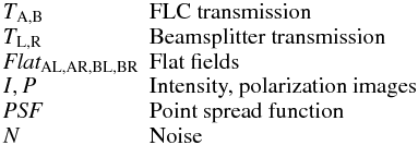 where TA,B accounts for the FLC transmission in its two possible states, and TL,R accounts for any transmission difference between the two beams. FlatAL,AR,BL,BR accounts for the different flat fields on the left and right sides of the CCD for the A and B images. The noise term includes the read-out and the photon noise. The polarization image includes any polarized light that enters the instrument, including sky polarization and polarization introduced by the telescope. The PSF can be expressed as the convolution of the “optics” and (PSFOpt) and “seeing” (S) terms of the PSF (e.g. Roddier 2004):
 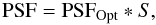 (1)where PSFOpt accounts for the static optical elements of the instrument and telescope, and S accounts for the dynamic atmosphere. Any small imperfection in the beamsplitter or difference in the optical path between the two beams will translate into different PSFOpt for the left and right images: PSFL and PSFR. On the other hand, the atmosphere will change with time, so S will also change for the A and B frames: SA and SB. Taking all of this into account, the four images recorded by the CCD in one FLC cycle can be described by
 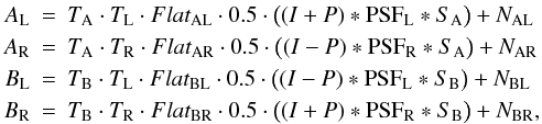 (2)where AL stands for the left image taken when the FLC is in its A state, and so on. NAL refers to the noise associated with this image. Symbols “·” and “*” stand for multiplication and convolution, respectively. The factor 0.5 comes from the beamsplitter: the total incoming beam is divided into two. A “pure” intensity image can then be generated by adding the left and right beams.
Once a data set is recorded, the FLC is rotated by 22.5°, and a new data set is acquired. Because ExPo does not have a derotator, the field rotation will rotate not only the image, but also the polarization plane of the incoming light. To avoid this, the images are calibrated according to the reference system of the observed target and are then transformed to the reference system of the instrument. The Stokes parameters Q and U are obtained after combining and calibrating (Rodenhuis et al., in prep.) four datasets with the FLC rotated by 0°, 22.5°, 45° and 67.5° (e.g. Patat & Romaniello 2006). Two FLC positions (0° and 22.5° or 45° and 67.5°) are necessary to produce calibrated images, so two redundant data sets are obtained after calibrating. Random errors (e.g., uncorrected cosmic rays, FLC ghosts) are removed by comparing these two data sets.
3. Image preparation
In this section we describe the initial reduction steps that must be applied to the raw data. Once the images are corrected for dark, flat, and smearing effects, they are ready to be aligned and combined as explained in Sects. 4 and 5.
3.1. Dark reduction
A dark image is an image taken with a given exposure time and with the CCD shutter closed. However, this is not possible because of the short exposure times required by ExPo, as we will explain in the next subsection, and the CCD shutter must remain open during the whole observation. An opaque filter is placed in the filter wheel to measure dark frames.
Every dark frame is checked to detect and remove cosmic rays (CR). They are identified as pixels showing values higher than a threshold value. This threshold is defined according to the characteristics of the dark observation, i.e., dark frames obtained with different CCD gain values will require different threshold values to detect the CR events. This process produces good results when reducing dark frames. Another approach is used when reducing the final science images, as is explained in Sect. 3.4. Finally, a very low-noise master dark is generated by combining at least 8000 dark frames (equivalent to a total integration time of roughly 4 min).
3.2. Smearing and second-order corrections
Owing to the short exposure times used by ExPo, the CCD runs in frame-transfer mode, which means that the detector is reading and recording frames at the same time. To achieve this, the CCD chip is split in half: one half for exposing and another half for reading. Once an image is recorded on the “exposing” half, it is shifted to the read-out area. The shutter remains open during the whole process, and this, unfortunately, introduces spurious effects that must be removed in the initial reduction of the raw images.
Each time a frame is transferred to the read-out area of the CCD, there is some leftover charge. As a result of this, an extra background is added to the next recorded frame. Moreover, if the observed target is too bright, a streak in the direction of the charge shifting will appear when exposing for a long time, or averaging many short-exposure images.
Owing to the field mask, some areas of the CCD are not illuminated (Fig. 3). Any signal measured in these non-illuminated regions must come either from the extra background mentioned above or from the read-out noise. The information contained in these “dark” pixels is used to remove these two effects. An example of this is shown in Fig. 4: the spurious signal is first measured outside of the field mask, and then subtracted from the raw image.
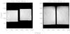 |
Fig. 3 Normalized flat fields with two different field masks. |
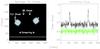 |
Fig. 4 Left: raw image, plotted at very high contrast. Two spurious ghosts can be seen above the star (discussed below in Sect. 6.4). The horizontal white line represents the plot that is shown on the right. Right: the black line shows the horizontal cut before the correction, the green line shows the smearing correction effect described in Sect. 3.2. |
3.3. Flat reduction
A set of dome flats is taken at the beginning and the end of each observing night. A minimum number of 100 frames are recorded for each of the four FLC positions (0°,22.5°,45°,67.5°). Every frame is then corrected for dark and smearing effects. As with the images, it is convenient to distinguish between FlatAL, FlatAR, FlatBL and FlatBR. Any polarization introduced by the dome lights, beamsplitter, and FLC transmission differences disappears when one normalizes each of these flats independently. All flat field images are combined to generate four master flats.
The analysis of the flat fields shows that the CCD has no dead pixels.
3.4. Cosmic ray correction
Before the images are combined and analyzed, they are corrected for cosmic rays. A standard ExPo data set comprises 20 000 images (around 10 min exposure time) per FLC position. The CR contribution cannot be neglected because we are dealing with contrast ratios of ≈ 105. Owing to the nature of the ExPo images, with very short exposure times and a FOV of 20′′ × 20′′, it is not trivial to distinguish between a real speckle and a CR. Standard CR rejection methods are based on comparing an average image with the individual ones, and then applying a sigma-rejection algorithm. However, the speckle pattern disappears in the average; the average and individual images are indeed quite different. A different approach, based on the advantage of having two simultaneous images in the same frame, is used in this analysis. A box of 5 × 5 pixels is extracted around the brightest pixel of the left and right images. The standard deviations (σ) of these two boxes are then compared. Experimental results show that if the brightest pixel corresponds to a CR and not to a speckle, its associated σ will be at least three times greater than the σ of a true speckle. Cosmic rays are detected and corrected according to this threshold: if one of the boxes contains a CR, all its pixels are set to the mean value of the whole image.
If both the left and right images are affected by CRs, this method will still work because the probability that the cosmic rays have the same standard deviation is very low. Fainter CR can be divided into two categories: those that fall inside the speckle pattern and those that fall outside of it. The former are, in practice, impossible to distinguish from true speckles. The latter are removed from the final images at the end of the analysis. Figure 5 shows an example of this process: one uncorrected CR appears in one set but not on the other, so it can be easily identified and removed from the final image.
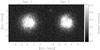 |
Fig. 5 Polarized images of AB Aurigae (seeing was ~1.4′′). Set 1 shows a calibrated image generated with the FLC placed at 0° and 22.5°. Set 2 shows the polarized image generated after placing the FLC at 45° and 67.5°. The white circle shows the position of a cosmic ray that does not appear in the first image. |
4. Image alignment
Once these corrections are applied, the images are aligned before they are combined. During the image acquisition, the telescope guides on the observed target (i.e., there is no reference star to be tracked). As a result of this, the accuracy of the guiding decreases, specially in the fainter (mv ≥ 9) targets. Because of the small field of view of ExPo, any small telescope misalignment can shift the image center by several pixels. Additionally, owing to the short exposures used, the PSF is a speckle pattern. All these contributions make image alignment one of the main sources of error in the processing of ExPo data. To reduce misalignment effects, two centering algorithms were tested: brightest speckle and template cross-correlation.
The brightest speckle-method (or shift-and-add method) is used in lucky imaging (e.g., Law et al. 2006). The images are aligned according to the position of the brightest speckle in every image.
The template cross-correlation method first requires a starting template or reference image. Once the template is provided, each single image is cross-correlated with it. The image center is now defined as the position of the maximum value of this operation. Different templates such as a simulated Gaussian-shaped point spread function (PSF) or an average speckle-centered real PSF were used in these calculations.
Once the images are centered, and before they are combined, they are again aligned to minimize any other source of misalignment, such as sub-pixel or flat-field gradients. These effects are corrected with a custom version of the drizzle code of Fruchter & Hook (2002). In this code, each pixel is expanded into several pixels, making it possible to shift and align images with sub-pixel accuracy.
The analysis shows that the best results are obtained when combining these three methods. First, a template is generated by centering each left and right image according to the brightest speckle. An average non-Gaussian shaped PSF is generated after combining all these images. Then, this PSF is used as the input template for the second method: each individual image is now cross-correlated with this template. Finally, each “right” image is aligned with respect to the “left” one by using the drizzle code. Each pixel is subdivided into nine sub-pixels, which results in an alignment accuracy of a third of a pixel. Any shift introduced by the FLC is also corrected by this centering process.
To check how misalignment affects the data reduction, several unpolarized (diskless) stars were analyzed. In these cases, no polarization pattern is expected to be measured. The accuracy of the alignment can be quantified in terms of the standard deviation σ of this pattern. Figure 6 shows the polarization pattern measured for the unpolarized star HD 122815. The top row shows the difference between the template-center and the speckle-center. The bottom row shows the same result, but now including sub-pixel alignment with a third of a pixel accuracy. The combination of template center plus sub-pixel alignment shows almost no structure at all (Fig. 6, lower-left corner).
From Fig. 6 it is clear that most of the misalignment disappears when aligning the images according to the cross-correlation method. No significant improvement is detectable when aligning with sub-pixel accuracy because of the lack of structure in a diskless star.
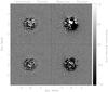 |
Fig. 6 Polarized (uncalibrated) results for a diskless (unpolarized) star: HD 122815. Four different alignment approaches are shown. Left column: images are aligned with a template. Right column: images re aligned according to the brightest speckle (shift-and-add). Top row: No sub-pixel alignment. Bottom row: sub-pixel alignment. Color bar: amount of (uncalibrated) polarization, P. |
5. Image combination
As described by Bagnulo et al. (2009), there are two methods of combining images produced with a dual-beam polarimeter to produce polarization images: one based on the image ratios and the other based on the image differences. For ExPo, these two approaches can be expressed in terms of Eq. (2) as  (3)for the double-ratio method, and as
  (4)for the double-difference method. Both methods were investigated. The results prove that better results are obtained when applying the double-difference method instead of the double-ratio explained in detail in Keller (1996) and Donati et al. (1997). This result is shown in Fig. 7, where the same data set was reduced applying the double-differences method (left) and the double-ratio method (right). This can be explained by the difference of the speckle pattern for each image. Even though AL and AR are recorded simultaneously, they show small differences in their speckle patterns from instrumental effects. Owing to the huge dynamic range of our images, the slightest difference between two images will produce a big effect when calculating a ratio. However, the difference method is less sensitive to this. Therefore, this method was chosen for ExPo.
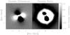 |
Fig. 7 AB Aurigae images obtained after applying the double difference (left) and double ratio (right). Color Bar: amount of (uncalibrated) polarization, P. |
At this point the dual-beam + beam-exchange technique shows its advantages. The combination of the four images generated in each FLC cycle minimizes the systematic errors. Following the notation introduced in Sect. 2, all terms that appear when developing the equations are listed in Table 1.
Notation used during the development of the image analysis.
Once the images are corrected for dark, flat, and smearing effects, the following differences can be defined:  where δI and δP refer to differences between the left and right beams. The difference between TL and TR produces a bias between left and right images, while the difference between PSFL and PSFR differentially distorts the images. If the beamsplitter does not produce two identical beams (i.e., from optical imperfections) δI will be non-zero. Because ExPo looks for polarized intensities of P ≈ 10-5I, this term should be on the order of ≈ 10-4 or smaller, as will be explained in the next paragraphs. As soon as this condition is not satisfied, the polarization values will be affected by the uncorrected intensity differences.
To evaluate the effect of δI on the polarimetry results, two average intensity “left” and “right” images were produced by averaging left and right beams: IL = AL + BL,IR = AR + BR. Both images were aligned with a third of a pixel accuracy, then normalized, and finally subtracted. The noise contribution can be neglected in this calculation because its contribution is several orders of magnitude below the intensity level. The result is described by  (7)where δ′I and δ′P refer to any difference between the A and B frames. The difference between TA and TB will affect the whole image like a bias value, and the difference between SA and SB will affect the image shape. The later will be averaged out when combining enough images, i.e., the seeing effect will affect the A and B frames in the same way. Ferroelectric liquid crystal transmission differences are not higher than 10-3 for our current FLC (Rodenhuis et al., in prep.), therefore δ′I ≈ 10-3, and δ′P will be very close to unity δP ≈ 1. Taking all of this into account, the first term of Eq. (7) is much larger than the second term: I ∗ δ′P ≫ P ∗ δ′I, so Eq. (7) becomes
  (8)Figure 8 illustrates this result for the diskless star HD 122815, observed with the FLC oriented at 0°. The image is scaled to its maximum, i.e., the beam differences have an amplitude of ≈ ± 4 × 10⁻⁴, which means that this is the magnitude of δI. Similar values are found when repeating this experiment for different FLC orientations.
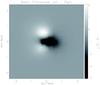 |
Fig. 8 Normalized difference between left and right beams. The asymmetrical pattern around the center means shape differences (i.e., PSFL and PSFR produce different patterns). The color bar is in units of 10-4, meaning that this is the magnitude of the beam differences. |
As can be clearly seen from these results, beamsplitter imperfections are an important effect that needs to be taken into account when dealing with contrast ratios of 104 or higher. Any differences in the PSF of each beam can modify the final result when aiming for such high contrast ratios. This contribution is, however, minimized when working with the double-difference method: 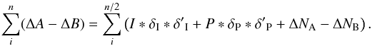 (9)In this case, the four images produced in each FLC cycle are first combined, and then averaged over the whole data set. Now the intensity term is convolved with the convolution of δI and δ′I. The latter will have a magnitude of δI ∗ δ′I ≈ 10-7, so the intensity will be decreased by this factor. Both δP and δ′P are close to unity, so their convolution will be also close to unity. The polarization term is then neither increased nor decreased. Finally, the noise term is not modulated by any delta factor. Its contribution is minimized by the double-difference and it will be averaged out. This term will define the maximum contrast attainable with ExPo.
Figure 9 summarizes the previous results for both a diskless star (HD 122815) and a protoplanetary disk (AB Aurigae). The first two columns starting from the left show the result given by Eqs. (5) and (6), respectively, when applied to these two targets. The result of a single-beam experiment is shown in the third column. In this case, the images produced by just one beam (the right one) are shown for comparison. The result of the double-difference described by Eq. (9) is shown in the right column. In the first and second columns the polarization pattern is contaminated by the intensity term described by δI, and the third column shows that the images are more noisy. The fourth column has no artifacts, showing a clean polarization pattern, with the lowest noise level.
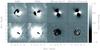 |
Fig. 9 Uncalibrated polarized image. Top rows: AB Aurigae. Bottom rows: unpolarized star. Color bar: (uncalibrated) polarization, P (arbitrary units). The results plotted in the left and center columns are contaminated by instrumental artifacts. These artifacts are minimized when applying the double-difference, as is shown in the right column. |
6. Additional corrections
6.1. Instrumental polarization
The polarized light measured by ExPo not only contains the polarized light coming from the circumstellar environment, but also telescope polarization (Miller 1963) and interstellar polarization (Hiltner 1949). Moreover, any small difference between the beamsplitter transmission coefficients (TA,TB) or the FLC transmission coefficients (TL,TR) introduces an artificial polarization signature. All these contributions are proportional to the intensity of the incoming light, so their effects can be measured by measuring the degree of polarization at the center of the (largely unpolarized) star. The polarization compensator used by ExPo minimizes these effects, but there is always some leftover instrumental polarization. Taking into account that AL + AR ≈ TA·SA ∗ I ∗ δP, and BL + BR ≈ TB·SB ∗ I ∗ δP, the polarization degree at the star’s center for the A frame can be described as 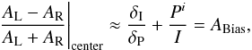 (10)and for the B frame:
 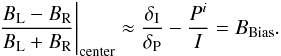 (11)Pi refers to any polarization feature that does not come from the circumstellar environment. As explained in Rodenhuis et al. (in prep.), the polarization compensator is working for all observations (including unpolarized diskless stars), and it is impossible to set a true zero or reference level for our polarimetric observations. Therefore, all calculations are based on the assumption that the starlight is unpolarized. However, this is not true if there is strong inner disk polarization (Min et al., in prep.). In these cases, a degree of polarization on the order of a few per cent is expected to be measured at the star’s position. On the other hand, the expected instrumental polarization is a few percent as well, so in practice it is impossible to distinguish inner disk polarization from instrumental polarization. The ABias and BBias are then subtracted from the degree of polarization for the A and B frames:
 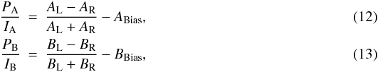 where dPA and dPB are the instrumental polarization-corrected degree of polarization for the A and B frames, respectively. The (uncalibrated) polarization image PA is then calculated as the product of the degree of polarization times the intensity:
 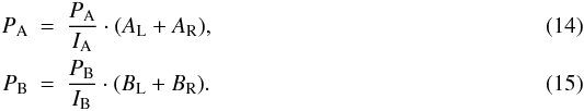 Figure 11 shows the effect of this correction. An artificial bias appears in the polarization images when the IP correction is not applied. If the star is unpolarized (bottom row), a bias level appears as a consequence of the imperfect compensation. In the case of AB Aur (top row) the polarization pattern is distorted when no correction is applied.
 |
Fig. 10 Polarization degree for the unpolarized (diskless) star HD122815 (left), and for AB Aurigae (right). |
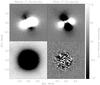 |
Fig. 11 Effect of the instrumental polarization (IP) on the final images. Top: AB Aurigae. Bottom: unpolarized star. Color bar: polarization (P), arbitrary units. |
6.2. Field rotation
All alt-azimuth telescopes are affected by field rotation. This term describes the amount of sky rotation, and it depends on the altitude (h) and azimuth (a) of the observed target, as well as on the latitude (φ) of the observer. It will reach its maximum value when pointing toward the zenith, and it will be almost negligible when pointing to very low altitudes. If the observations are made at the Nasmyth focus, an extra rotation must be taken into account, caused by the relative rotation between the telescope tube and the Nasmyth platform (see Marois et al. 2006; Joos 2007, Chap. 4): 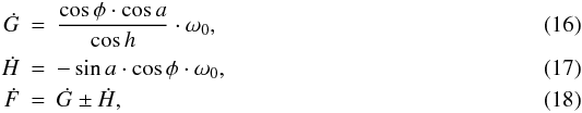 were ω0 is the sidereal rate. Ġ represents the rotation rate caused by the sky movement, and Ḣ accounts for the rotation rate caused by the telescope movement. Equation (18) is the total amount of field rotation rate at the Nasmyth platform. The ± is related to the two platforms at the telescope. In the case of ExPo, the instrument has been placed at the “B” platform of the William Herschel Telescope, so the “+” applies.
While most of the instruments incorporate a de-rotator to remove this effect, the design of ExPo does not include one. It is necessary to calculate Ḟ and then numerically rotate each observed target. Owing to the short exposure time of the ExPo images, the amount of de-rotation between one image and the next image is too small to correct (≤0.5°), so rotating each frame individually is not necessary. A rotation per image blocks is performed instead. Ḟ is assumed to be constant within a certain interval. If the observed target is not close (≤15°) to the Zenith, this interval can be set to 30 s. Otherwise, shorter time intervals must be taken to minimize errors. Different rotation routines were tested. To test this, different template images were first rotated and then de-rotated by using different codes. The standard deviation σ of the difference between the original template and the de-rotated version is a measurement of the accuracy of the rotation procedure. This analysis shows that the best results are obtained when the image is first resampled to one fifth of a pixel. The rotation is then performed with the IDL routine rot, using cubic interpolation, with the interpolation parameter set to − 0.7.
6.3. Sky-background polarization
The polarization of the sky (Bailey et al. 2008) is variable, depending on the position of the target as well as the position of the Moon (because scattered moonlight is polarized). Unlike the instrumental polarization discussed in Sect. 6.1, this contribution does not depend on the brightness of the observed target, but it behaves like a polarization bias over the whole image. Therefore, the background polarization cannot be calculated by measuring the degree of polarization at the star’s center. The background polarization is subtracted at the very last stage of the data analysis by measuring the polarization in the sky regions of the image. The median value of at least four different sky regions is calculated and subtracted from the reduced polarization images.
6.4. Ghosts
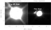 |
Fig. 12 Intensity images of the same star observed without (left) and with (right) Hαcont filter. The images are plotted at different contrast to enhance the ghost image. The diffraction caused by the telescope spiders is clearly visible in the left image. |
Three different sources of optical ghosts are identified in ExPo: the filters, the beamsplitter and the FLC. While the latter produces ghosts that move according to the FLC angle, the ghosts produced by filters and the beamsplitter remain in a fixed position (an example of these ghosts can be seen in Fig. 12). Filter ghosts are minimized by tilting the filters. All these ghosts appear are contrast ratios of 10-4.
To analyze the effects caused by the ghosts on the polarized images, the mean and standard deviation (σ) was calculated around the position of the ghosts and around sky (empty) regions in the polarization images. This test was performed for several (ghost-affected) images, with the result that it is impossible to distinguish between ghosts and sky regions when looking at the polarized images, i.e., ghosts do not contribute to the polarization image any more than the sky background. However, special care has to be taken when looking at the degree of polarization of the images. In this case, because the ghost appears in intensity (at contrast ratios of ~10-4), it can contribute to the degree of polarization.
7. Discussion
Flat-field errors (i.e., pixel-to-pixel sensitivity variations) are not limiting ExPo. Because each image is shifted individually before averaging, flat-field effects are averaged out. However, flat-field effects might play an important role when an AO system is added to the instrument. In this case, the PSF is expected to remain in a fixed position on the CCD, with no need to re-center the images.
Brightest-speckle alignment is not as good as template-alignment for our images. This result, which disagrees with previous work (Law 2006; Christou 1991), can be explained by the characteristics of this instrument. The small field of view used by ExPo combined with the four different PSFs generated in each FLC cycle makes a big difference with respect to the standard lucky-imaging observations. The speckle pattern produced by a single star is distributed over several pixels, and the beam differences make this pattern to be slightly different in the left and right images, even though they correspond to simultaneous observations. As a result of this, the brightest speckle on the left image is not necessarily the same as the brightest speckle on the right image. Therefore, the template center method produces better results than the speckle center method. However, in case of good seeing (below 0.7′′), both methods converge, leading to very similar results. This can be explained by taking into account that in those cases, the PSF peak is concentrated in very few pixels, so the region covered by the speckle pattern is very small. Under these conditions, the center defined by the template-center method and the brightest speckle are about the same.
While theoretically both the ratio and the difference method should produce similar results, this analysis shows that the first one fails when applied to a dual-beam imaging polarimeter like ExPo. The photon noise variance is signal-dependent, i.e., it is proportional to the amount of photons in each image. On the other hand, each image produced by this instrument is affected by a different combination of beamsplitter and FLC transmission coefficients, which means that the total amount of light in each of the four images produced in one FLC cycle is slightly different. This also applies to the photon noise, resulting in different levels of noise in each image. The double-difference minimizes this effect, while the dual-ratio can increase it. This is a particular result for this experiment, but it can be generalized to any dual-beam polarimeter.
Numerical simulations show that the bias correction described in Sect. 6.1 must be applied even when there is no instrumental polarization (Min et al., in prep.). The strong polarization produced by the inner rim of a protoplanetary disk dominates the polarized intensity, making it much harder to detect the remaining circumstellar polarization.
As mentioned in Sect. 2, future versions of ExPo may make use of 3 FLCs in a Pancharatnam configuration to minimize the chromatic effects introduced by the current single-FLC configuration. This change will not affect the current data-reduction process, but it will improve the instrument polarimetric performance.
The inclusion of an AO system in ExPo will lead to a much sharper PSF. The amount of speckles in these new PSFs will be considerably smaller than in our current PSFs. Real speckle-sized polarized features (i.e., exoplanets) might be removed as a result of the current CR rejection algorithm. One possible solution to this problem might be a new technique based on the comparison of the two differences (ΔA and ΔB) described by Eqs. (5) and (6). A polarized speckle-sized feature such as an exoplanet is expected to appear in both images at the same coordinates, while in case of a CR, it will appear in only one of these differences.
Chromatic effects introduced by the FLC and the BS are out of the scope of this paper, but must be taken into account in future instruments such as SPHERE or EPICS.
Finally, lucky-imaging techniques (i.e., frame selection) do not produce significant improvements in our observations because the standard exposure time for a target is around one hour (around 20 min per FLC position). In this regime, the amount of “lucky images” is not enough to produce a good signal-to-noise ratio.
8. Conclusion
Dual-beam polarimeters are becoming more and more popular among the astronomical community, such as the ones described by Packham et al. (2005), Masiero et al. (2008) and Nagaraju et al. (2008). The high contrast ratios achieved by polarimetry make this technique a promising tool to characterize exoplanets as well as circumstellar environments.
ExPo can currently reach contrast ratios of 105 at a four-meter class telescope by means of polarimetry. As we showed in this analysis, instrumental artifacts can be minimized by properly combining the data produced by a dual-beam instrument. The template-centering method produces better results than the speckle-centering method. The main limitations of the instrument are the beamsplitter imperfections and the FLC transmission differences, as explained in Sect. 5. Future versions of this instrument will include an adaptive optics system as well as a coronagraph, which will require new approaches to the data reduction.
Acknowledgments
We are grateful to the staff at the William Herschel Telescope for their support when commissioning of ExPo. We also thank the referee for his/her useful comments and recommendations.
References
- Bagnulo, S., Landolfi, M., Landstreet, J. D., et al. 2009, PASP, 121, 993 [NASA ADS] [CrossRef] [Google Scholar]
- Bailey, J., Ulanowski, Z., Lucas, P. W., et al. 2008, MNRAS, 386, 1016 [NASA ADS] [CrossRef] [Google Scholar]
- Christou, J. C. 1991, PASP, 103, 1040 [NASA ADS] [CrossRef] [Google Scholar]
- Donati, J., Semel, M., Carter, B. D., Rees, D. E., & Collier Cameron, A. 1997, MNRAS, 291, 658 [NASA ADS] [CrossRef] [MathSciNet] [Google Scholar]
- Fruchter, A. S., & Hook, R. N. 2002, PAJP, 114 [Google Scholar]
- Graham, J. R., Macintosh, B., Doyon, R., et al. 2007, in BAAS, 38, 968 [Google Scholar]
- Hiltner, W. A. 1949, Science, 109, 165 [NASA ADS] [CrossRef] [Google Scholar]
- Hook, I. 2009, in Science with the VLT in the ELT Era, ed. A. Moorwood, Astrophys. Space Sci. Proc. (The Netherlands: Springer), 225 [Google Scholar]
- Joos, F. 2007, Ph.D. Thesis, Eidgenoessische Technische Hochschule Zuerich, Switzerland [Google Scholar]
- Kalas, P., Graham, J. R., Chiang, E., et al. 2008, Science, 322, 1345 [NASA ADS] [CrossRef] [PubMed] [Google Scholar]
- Kasper, M., Beuzit, J., Verinaud, C., et al. 2010, SPIE Conf. Ser., 7735 [Google Scholar]
- Keller, C. U. 1996, Sol. Phys., 164, 243, [NASA ADS] [CrossRef] [Google Scholar]
- Keller, C. U. 2002, Instrumentation for Astrophysical Spectropolarimetry [Google Scholar]
- Kuhn, J. R., Potter, D., & Parise, B. 2001, ApJ, 553, L189 [NASA ADS] [CrossRef] [Google Scholar]
- Lagrange, A.-M., Bonnefoy, M., Chauvin, G., et al. 2010, Science, 329, 57 [NASA ADS] [CrossRef] [PubMed] [Google Scholar]
- Law, N. M. 2006, Ph.D. Thesis, Cambridge University [Google Scholar]
- Law, N. M., Mackay, C. D., & Baldwin, J. E. 2006, A&A, 446, 739 [NASA ADS] [CrossRef] [EDP Sciences] [Google Scholar]
- Marois, C., Lafrenière, D., Doyon, R., Macintosh, B., & Nadeau, D. 2006, ApJ, 641, 556 [Google Scholar]
- Marois, C., Macintosh, B., Barman, T., et al. 2008, Science, 322, 1348 [NASA ADS] [CrossRef] [PubMed] [Google Scholar]
- Martinez, P., Carpentier, E. A., & Kasper, M. 2010, PASP, 122, 916 [NASA ADS] [CrossRef] [Google Scholar]
- Masiero, J., Hodapp, K., Harrington, D., & Lin, H. 2008, in Astronomical polarimetry 2008, Science from small to large telescope, ed. P. Bastien, ASP Conf. Ser., in press [arXiv:0809.4313] [Google Scholar]
- Miller, R. H. 1963, Appl. Opt., 2, 61 [NASA ADS] [CrossRef] [Google Scholar]
- Nagaraju, K., Sankarasubramanian, K., Rangarajan, K. E., et al. 2008, BASI, 36, 99 [NASA ADS] [Google Scholar]
- Packham, C., Hough, J. H., & Telesco, C. M. 2005, in Astronomical Polarimetry: Current Status and Future Directions, ed. A. Adamson, C. Aspin, C. Davis, & T. Fujiyoshi, ASP Conf. Ser., 343, 38 [Google Scholar]
- Pancharatnam, S. 1955, Proc. Math. Sci., 41, 130 [Google Scholar]
- Patat, F., & Romaniello, M. 2006, PASP, 118, 146 [NASA ADS] [CrossRef] [Google Scholar]
- Roddier, F. 2004, Adap. Opt. Astron., ed. F. Roddier [Google Scholar]
- Rodenhuis, M., Canovas, H., Jeffers, S. V., & Keller, C. U. 2008, SPIE Conf. Ser., 7014 [Google Scholar]
- Stam, D. M., Hovenier, J. W., & Waters, L. B. M. F. 2005, in Astronomical Polarimetry: Current Status and Future Directions, ed. A. Adamson, C. Aspin, C. Davis, & T. Fujiyoshi, ASP Conf. Ser., 343, 207 [Google Scholar]
- Stam, D. M., Laan, E., Selig, A., Hoogeveen, R., & Hasekamp, O. 2006, in European Planetary Science Congress 2006, 607 [Google Scholar]
- Thalmann, C., Schmid, H. M., Boccaletti, A., et al. 2008, SPIE Conf. Ser., 7014 [Google Scholar]
- Todorov, K., Luhman, K. L., & McLeod, K. K. 2010, ApJ, 714, L84 [NASA ADS] [CrossRef] [Google Scholar]
- Wynne, C. G. 1993, MNRAS, 262, 741 [NASA ADS] [Google Scholar]
All Tables
All Figures
|
Fig. 1 Pipeline Block Diagram. |
| In the text | |
|
Fig. 2 Schematic layout of the instrument in the Nasmyth focus of a telescope. |
| In the text | |
|
Fig. 3 Normalized flat fields with two different field masks. |
| In the text | |
|
Fig. 4 Left: raw image, plotted at very high contrast. Two spurious ghosts can be seen above the star (discussed below in Sect. 6.4). The horizontal white line represents the plot that is shown on the right. Right: the black line shows the horizontal cut before the correction, the green line shows the smearing correction effect described in Sect. 3.2. |
| In the text | |
|
Fig. 5 Polarized images of AB Aurigae (seeing was ~1.4′′). Set 1 shows a calibrated image generated with the FLC placed at 0° and 22.5°. Set 2 shows the polarized image generated after placing the FLC at 45° and 67.5°. The white circle shows the position of a cosmic ray that does not appear in the first image. |
| In the text | |
|
Fig. 6 Polarized (uncalibrated) results for a diskless (unpolarized) star: HD 122815. Four different alignment approaches are shown. Left column: images are aligned with a template. Right column: images re aligned according to the brightest speckle (shift-and-add). Top row: No sub-pixel alignment. Bottom row: sub-pixel alignment. Color bar: amount of (uncalibrated) polarization, P. |
| In the text | |
|
Fig. 7 AB Aurigae images obtained after applying the double difference (left) and double ratio (right). Color Bar: amount of (uncalibrated) polarization, P. |
| In the text | |
|
Fig. 8 Normalized difference between left and right beams. The asymmetrical pattern around the center means shape differences (i.e., PSFL and PSFR produce different patterns). The color bar is in units of 10-4, meaning that this is the magnitude of the beam differences. |
| In the text | |
|
Fig. 9 Uncalibrated polarized image. Top rows: AB Aurigae. Bottom rows: unpolarized star. Color bar: (uncalibrated) polarization, P (arbitrary units). The results plotted in the left and center columns are contaminated by instrumental artifacts. These artifacts are minimized when applying the double-difference, as is shown in the right column. |
| In the text | |
|
Fig. 10 Polarization degree for the unpolarized (diskless) star HD122815 (left), and for AB Aurigae (right). |
| In the text | |
|
Fig. 11 Effect of the instrumental polarization (IP) on the final images. Top: AB Aurigae. Bottom: unpolarized star. Color bar: polarization (P), arbitrary units. |
| In the text | |
|
Fig. 12 Intensity images of the same star observed without (left) and with (right) Hαcont filter. The images are plotted at different contrast to enhance the ghost image. The diffraction caused by the telescope spiders is clearly visible in the left image. |
| In the text | |
Current usage metrics show cumulative count of Article Views (full-text article views including HTML views, PDF and ePub downloads, according to the available data) and Abstracts Views on Vision4Press platform.
Data correspond to usage on the plateform after 2015. The current usage metrics is available 48-96 hours after online publication and is updated daily on week days.
Initial download of the metrics may take a while.