| Issue |
A&A
Volume 531, July 2011
|
|
|---|---|---|
| Article Number | A87 | |
| Number of page(s) | 12 | |
| Section | Extragalactic astronomy | |
| DOI | https://doi.org/10.1051/0004-6361/201116687 | |
| Published online | 20 June 2011 | |
Is the far border of the Local Void expanding?⋆,⋆⋆
1 Okayama Astrophysical Observatory, National Astronomical Observatory of JapanHonjo, Kamogata, Asakuchi Okayama 719-0232 Japan
This email address is being protected from spambots. You need JavaScript enabled to view it.
2 Observatoire de Paris – Meudon, GEPI, 92195 Meudon Cedex, France
Received: 10 February 2011
Accepted: 14 April 2011
Abstract
Context. According to models of evolution in the hierarchical structure formation scenarios, voids of galaxies are expected to expand. The Local Void (LV) is the closest large void, and it provides a unique opportunity to test observationally such an expansion. It has been found that the Local Group, which is on the border of the LV, is running away from the void center at ~260 km s-1.
Aims. In this study we investigate the motion of the galaxies at the far-side border of the LV to examine the presence of a possible expansion.
Methods. We selected late-type, edge-on spiral galaxies with radial velocities between 3000 km s-1 and 5000 km s-1, and carried out HI 21 cm line and H-band imaging observations. The near-infrared Tully-Fisher relation was calibrated with a large sample of galaxies and carefully corrected for Malmquist bias. It was used to compute the distances and the peculiar velocities of the LV sample galaxies. Among the 36 sample LV galaxies with good quality HI line width measurements, only 15 galaxies were selected for measuring their distances and peculiar velocities, in order to avoid the effect of Malmquist bias.
Results. The average peculiar velocity of these 15 galaxies is found to be  km s-1, which is not significantly different from zero.
Conclusions. Due to the intrinsically large scatter of Tully-Fisher relation, we cannot conclude whether there is a systematic motion against the center of the LV for the galaxies at the far-side boundary of the void. However, our result is consistent with the hypothesis that those galaxies at the far-side boundary have an average velocity of ~260 km s-1 equivalent to what is found at the position of the Local Group.
Key words: galaxies: distances and redshifts / large-scale structure of Universe
Based on data taken at Nançay radiotelescope operated by Observatoire de Paris, CNRS and Université d’Orléans, Infrared Survey Facility (IRSF) which is operated by Nagoya university under the cooperation of South African Astronomical Observatory, Kyoto University, and National Astronomical Observatory of Japan.
This publication makes use of data products from the Two Micron All Sky Survey, which is a joint project of the University of Massachusetts and the Infrared Processing and Analysis Center/ California Institute of Technology, funded by the National Aeronautics and Space Administration and the National Science Foundation.
Present address: Subaru Telescope, National Astronomical Observatory of Japan, 650 North A’ohoku Place, Hilo, HI 96720, USA.
© ESO, 2011
1. Introduction
Deep extended galaxy surveys have shown that the large-scale distribution of galaxies consists in matter concentrations, such as clusters, filaments, and walls, and also in vast regions devoid of galaxies, i.e. the voids. These voids occupy the largest volumes in the Universe, according to Ceccarelli et al. (2006), and the radii of the voids those authors find in the 2dF galaxy redshift survey range from 5 to 25 h-1 Mpc (h = H0/100).
Voids are expected to expand, since galaxies undergo a gravitational pull at their borders from the objects located outside them. Sheth & van de Weygaert (2004) have developed a model of the evolution of voids, which indeed leads to an expansion of the surviving voids at the present time. On the other hand, Ceccarelli et al. (2006) have modeled the velocity field around the voids found in their study, and show that the expansion velocity is maximum at the edge of the voids and is proportional to the void radius, for instance reaching 210 km s-1 for a void with a radius of 12.5 h-1 Mpc.
It is also possible to directly measure the expansion velocities at the edge of a peculiar void, namely the Local Void (LV), taking advantage of its being very close to us. The LV was discovered by Tully & Fisher (1987) from their survey of galaxies with redshift lower than 3000 km s-1. Its structure has been investigated by Nakanishi et al. (1997) from a visual search of IRAS galaxies behind the Milky Way, since the major part of this void is at galactic latitude |b| < 15°. They localize its center at ℓ = 60°, b = −15°, cz = 2500 km s-1, and they find that it extends to cz = 5000 km s-1. On the other hand, the Local Group and neighboring galaxies are located at the boundary of the LV, as shown by Tully et al. (2008).
By accurate measurements of distances of 200 galaxies within 10 Mpc carried out with the Hubble Space Telescope, Tully et al. (2008) find that the Local Group and its neighboring galaxies are running away from the center of the LV with a velocity of 259 km s-1. This proves the expansion of the LV at our location and also solves the problem of the so-called “Local Velocity Anomaly” appearing in the motion of the LG relative to the CMB (Faber & Burstein 1988; Burstein 2000).
In the present study, we intend to determine the peculiar velocities of galaxies located at the edge of the LV opposite to us (cz ~ 3000−5000 km s-1) in order to check whether the LV also undergoes an observable expansion in that region. The peculiar velocities are computed from the distances of the galaxies measured by means of the near-infrared Tully-Fisher relation (hereafter IRTFR) using near-infrared and HI 21-cm observations.
The organization of the paper is the following. Section 2 presents the sample of the LV galaxies observed. And then the IR and HI measurements are described and the data of interest are given. In Sect. 3, the IRTFR in H-band is determined from a calibration sample and corrected for Malmquist bias. In Sect. 4 we compute the distances of the LV galaxies from the IRTFR and derive their peculiar velocities after correction of the observed radial velocities from infall into some nearby mass concentrations. Concluding remarks are given in Sect. 5.
2. Observations
2.1. The sample selection
We selected uniquely spiral galaxies for the HI and IR observations, since the TF relation is only valid for them. These objects were chosen as located at the edge of the LV opposite to us and slightly beyond, at galactic coordinates: 30° < l < 70°, |b| < 20° (i.e., around the North Supergalactic Pole), and with recession velocities cz < 5000 km s-1 (see the maps by Nakanishi et al. 1997). In addition to the galaxies in the literature (most of them are listed in the UGC catalog, Nilson 1973), we executed the redshift measurement observations for some galaxies that were discovered in a systematic optical search by Roman et al. (2000). The observations were done in July and October 2000 using the New Cassegrain Spectrograph attached to the 188 cm reflector of the Okayama Astrophysical Observatory, National Astronomical Observatory of Japan. In Table 1 we list these new radial velocities. Among these galaxies with new radial velocity measurements, those at cz < 5000 km s-1 were added to the sample, except UGC 11417, which does not satisfy the limit of the axial ratio (less than 0.71; see below).
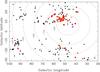 |
Fig. 1 Spatial distribution of the Local Void sample galaxies in galactic coordinates. Small filled circles represent galaxies in the IRAS PSCz catalog (Saunders et al. 2000) with radial velocity between 3000 km s-1 and 5000 km s-1. Larger circles are the Local Void sample galaxies in this study (50 galaxies, see Sect. 2.1). Filled circles are for the 36 galaxies included in the final sample (see Sect. 2.3), while open circles are those not in the final sample. Dashed lines indicate latitudes in the supergalactic coordinates, and the cross shows the position of the North supergalactic pole. The position opposite to the Local Velocity Anomaly defined by Burstein (2000) is indicated by a blue asterisk. |
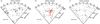 |
Fig. 2 Distribution of the Local Void sample galaxies in the galactic longitude – radial velocity planes. a)−c) display the galaxies with galactic latitude −30° < b < 0°, 0° < b < 20° and 20° < b < 40°, respectively. The meaning of symbols are the same as in Fig. 1: filled circles represent galaxies in the IRAS PSCz catalog (Saunders et al. 2000) with radial velocities. Larger circles are the 50 Local Void sample galaxies in this study. Larger filled circles are for the 36 galaxies included in the final sample, and open circles are those not in the final sample. |
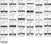 |
Fig. 3 The HI 21 cm line profiles of the 30 Local Void galaxies detected with Nançay radiotelescope and of the possibly detected one (UGC 11198). The horizontal axis is the radial velocity in km s-1 and the vertical axis is the flux density in mJy. The hanning and boxcar smoothing are applied and the subtraction of the polynomial fitted baseline is made. |
Use of the TF relation needs the determination of the maximal rotational velocity Vm of each galaxy, and Vm is obtained from the width W of the 21-cm HI profile by Vm ~ W/(2sini), where i is the inclination of the galaxy. To obtain accurate Vm, we only kept galaxies with i > 45deg, i.e., galaxies with axial ratios in the three-band coadded images in the Two Micron All Sky Survey (2MASS; Skrutskie et al. 2006), named “sup-ba” in the extended source catalog (XSC) less than 0.71 (assuming an intrinsic axis ratio of 0.2 for a spiral galaxy viewed edge-on).
Moreover, we need good S/N in the HI profiles to obtain good HI widths, hence accurate distances by the TF relation. Since the HI fluxes of the spiral galaxies are proportional to the square of their apparent diameters, such an accuracy is obtained by selecting only galaxies with sufficiently large apparent diameters. Taking into account the sensitivity of the Nançay radiotelescope, we kept mainly galaxies having an extinction-corrected major axis larger than one arcmin.
Finally, our observational sample comprises 50 galaxies with measured redshifts. In Figs. 1 and 2 we show the spatial distribution of these galaxies. It is shown in these figures that the sample galaxies well represent the population of the far-side boundary of the LV.
List of galaxies with new heliocentric radial velocity Vh measurements in km s-1 in the catalog of Roman et al. (2000).
2.2. HI 21-cm line observations
The 21-cm line observations of the LV galaxies were carried out with the Nançay radiotelescope. This instrument is a meridian one, with a half-power beam width at 21-cm of 3.6 arcmin (E-W) × 22 arcmin (N-S) at zero declination (nearly the same value for our galaxies, declinations of which are between + 10deg and + 25deg). The system temperature is 35 K. We used a bandwidth of 25 MHz covered by 2048 channels of the spectrometer, resulting in a velocity resolution of 2.6 km s-1. The observations were performed in an on-off mode, and the integration time on each galaxy generally ranged from 1 to 2 h.
Forty-three galaxies of our sample were observed between the years 2000 and 2004, leading to 30 detections, one possible detection and 12 non-detections. The line profiles of the detected galaxies were reduced using a hanning and boxcar smoothing, leading to a final velocity resolution of 2.6 × 4 = 10.4 km s-1. The line profiles of the detected galaxies and of the possibly detected one (UGC 11198) are shown in Fig. 3, after the hanning and boxcar smoothing and the subtraction of the polynomial fitted baseline. The parameters of interest derived from the profile were obtained, namely the widths W20 and W50 of the profile at 20% and 50% of the peak intensity, the heliocentric velocity Vh, and the HI flux FH. All these quantities are given in Table 2, with other data for the galaxies that are useful for the present study. For five galaxies (UGC 11254, UGC 11285, CGMW5-05908, UGC 11323, and UGC 11426), observations were disturbed by the Sun. However, the line widths can be measured correctly. On the other hand, the profiles of IRAS 18340+1016 and NGC 6930 are confused, and their line widths cannot be measured, so these two galaxies are not listed in Table 2.
The list of the 12 undetected galaxies is the following: CGCG 114−006, CGCG 172−027, CGCG 201−043, CGMW5− 05619, FGC 2187, NGC 6586, NGC 6641, NGC 6658, UGC 11301, UGC 11353, UGC 11368, and UGC 11369.
Description of Table 2: Col. (1) Name of the galaxy. (2) Equatorial coordinates α, δ (2000). (3) Galactic coordinates ℓ, b. (4) Heliocentric radial velocity Vh in km s-1. (5) Major and minor axes ac and bc in arcmin measured at the isophotal level of 25 mag/arcsec2 in the B-band, and corrected for inclination and for galactic extinction (those data come from Hyperleda database). (6) Position angle in degrees, from UGC or 2MASS XSC when the galaxy is not included in the UGC. (7) Galactic dust attenuation in V-band, from the map by Schlegel et al. (1998). (8) and (9) Widths W20 and W50 of the HI line in km s-1 at 20% and 50% of its maximum height, respectively, uncorrected for velocity resolution, with their uncertainties (after Fouqué et al. 1990). (10) Measured HI flux FH, in Jy × km s-1, with its uncertainty: 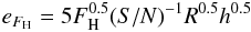 (1)where S/N is at the point of the profile of maximum intensity, R the resolution in km s-1, and h the peak intensity of the HI line (after Fouqué et al. 1990). (11) HI flux FH,c corrected for beam attenuation; f0 is the correction factor such that FH,c = f0FH. f0 is given by
  (2)where DH is the HI diameter of the galaxy, within which half of the HI mass is contained; DHEW is the projection of this diameter in the east-west direction, expressed in arcmin. One has DH = ac (after Hewitt et al. 1983). If θ is the position angle of the galaxy, its east-west corrected diameter is given by
  (3)Corrections for beam attenuation are small, only 3% on an average, except for NGC 6674 and IRAS 18575+1845, where they reach 20−30%. (12) Notes.
2.3. The final sample of galaxies measured in the HI line and selected for use in the IR TF relation
First we add to our initial sample of 30 detected galaxies 18 other galaxies located on the opposite border of the LV and measured elsewhere in the HI line (three of them, namely FCG 2187, UGC 11301 and UGC 11369 have not been detected by us). Thus we have a sample of 48 galaxies measured in the HI line at our disposal. One can note that 17 among our 30 detected galaxies have also been detected elsewhere (thus only 13 are newly measured by us).
In order to use the IRTFR in the best conditions, we need to have the best profile width W20. Thus we suppress all the cases of inaccurate W, of possible confusion, and of too narrow a profile corresponding to dwarf galaxies for which the TFR does not work correctly. There are 12 such galaxies, namely: UGC 11150, UGC 11253, UGC 11371, UGC 11552, IRAS 18340+1016, NGC 6930 (profile confusion), CGMW5−06653, CGCG 143−017, UGC 11333, UGC 11369 (too narrow or asymmetrical profile), CGMW5−05908 (W20 not accurate enough), and FCG 2187 (uncertain detection).
On the other hand, for galaxies measured by us and elsewhere as well, we have examined the two profiles obtained. If they were of equivalent quality, we took the average of the two values for W20 (after correction for velocity resolution). If one profile was much better than the other one, its W20 value was preferred.
Summary of the results of our HI 21 cm line observations with the Nançay radiotelescope.
Our final sample comprises 36 galaxies, namely, 19 galaxies for which our W20 or average of ours and others have been taken, four galaxies measured by us and others and for which the other W20 have been preferred, and 13 galaxies measured only elsewhere. The final values of W20 were corrected for velocity resolution R by  (Bottinelli et al. 1990). For our own measurements, the correction is −4.7 km s-1. These corrected W20 values are used to compute the widths corrected for inclination and redshift:
  used in IRTFR. The
  values are presented in Table 3.
Summary of the near-infrared photometry and corrected HI line widths for the final Local Void sample galaxies.
Description of Table 3: (1) name of the galaxy. (2) Equatorial coordinates α, δ (2000). (3) Galactic coordinates ℓ, b. (4) Heliocentric radial velocity Vh in km s-1. (5) Inclination of the galaxy in degrees. (6) H-band 20 mag/arcsec2 isophotal elliptical magnitude and its error. (7) H-band magnitude corrected for galactic and internal extinctions. (8) Source of H-band photometry. “UH88” and “IRSF” stand for photometry based on our own observations with the UH 2.2 m telescope and the IRSF 1.4 m telescope, respectively. “2MAS” stands for data taken from the 2MASS XSC. (9) Logarithm of the width of the HI line at 20% of its maximum height, corrected for velocity resolution, inclination, and redshift, in km s-1. (10) Logarithm of the maximum of the rotation velocity in km s-1, derived from log Wc. See text for details. (11) Source of HI line width data. “Nançay”: our own measurements. “Springob”: Springob et al. (2005). “LEDA”: the on-line galaxy database HyperLEDA (Paturel et al. 2003a). “Mean”: the average value of measurements by our observations at Nançay, HyperLEDA, and Springob et al. (2005) (when available).
2.4. Near-IR (H-band) observations and data reduction
Near-infrared (H-band) imaging observations were carried out using two facilities. One is the Quick Near-Infrared Camera (QUIRC) equipped to the University of Hawaii 2.2 m telescope (UH88) at Mauna Kea, Hawaii, and the other one is the near-infrared Simultaneous Infrared Imager for Unbiased Survey (SIRIUS: Nagashima et al. 1999; Nagayama et al. 2003) on board the Infrared Survey Facility (IRSF) telescope in the South African Astronomical Observatory (SAAO) at Sutherland, South Africa.
Observations with UH88/QUIRC were carried out in 2001 July 7−9 and August 4−5 (UT). The condition was mostly photometric throughout observing dates. QUIRC has a HAWAII 1024 × 1024 HgCdTe array with pixel scale of 0.19″/pixel, yielding a field-of-view of 193″ × 193″. Total on-source integration times range from 600 s to 1200 s, depending on the apparent surface brightness of objects.
Observations with IRSF/SIRIUS were made during 2003 March 31−April 4 and 2004 March 14−22. Although the SIRIUS camera has a capability of obtaining J, H, and Ks images simultaneously, in the present analysis only H-band images are used for the H-band Tully-Fisher relation. The field of view and the pixel scale of SIRIUS are  × and
× and  , respectively. Total on-source integration times are 900 s for UGC 11001 and CGMW5−06881, and 1200 s for UGC 11003.
Basic data reduction, including dark subtraction, flat-fielding, image alignment, and stacking, was done in a standard way using IRAF. Since the LV region is close to the Galactic plane, it is crowded with foreground stars. It is quite important to remove these stars before executing the photometry of target galaxies, for precise measurement of their apparent magnitude. For faint stars we did PSF fitting using Moffat profile for each star and subtracted them from reduced images. For bright stars their profiles are saturated, and we could not execute profile fitting. In that case we removed these stars by interpolation of counts from surrounding pixels using an IRAF task “IMEDIT”. After the removal of foreground stars, isophotal ellipses with H = 20 mag/arcsec2 were defined for each galaxy, and we calculated counts within the ellipse. Photometric zero points were derived for each night using near-infrared standard stars.
For 15 objects in our sample we could not obtain our own H-band imaging data. For these objects we used data in the 2MASS XSC. We used 20 mag/arcsec2 isophotal elliptical aperture magnitude (h_m_i20e) in the catalog. With the galaxies for which we obtained imaging data with UH88 and IRSF, we checked the consistency of the photometry between ours and the 2MASS XSC. For galaxies with relatively fewer foreground stars in the aperture (which can disturb the automated photometric procedure adopted in the 2MASS XSC), we found that the difference between our isophotal magnitudes and those in 2MASS XSC is less than 0.1 mag in most cases. In Table 3 we list the results of H-band photometry for the final sample galaxies.
3. Near-infrared Tully-Fisher relation
We use the Tully-Fisher relation (TFR) to compute the distances of the LV sample galaxies. We first proceed here to determine the TFR in the H-band. Generally speaking, the Tully-Fisher relation (TFR) is an empirical linear relationship between the logarithm of the maximum rotational velocity Vm of any spiral galaxy and its absolute magnitude M, namely,  (4)where a and b are constant quantities in a given system of magnitudes (Tully & Fisher 1977), and Vm can be determined from the width W of the 21-cm HI line or from the optical rotation curve. This relationship is a powerful and accurate distance indicator for the spiral galaxies and has been extensively used for such a purpose (e.g., Sakai et al. 2000). In the present study it is critically important to use near-infrared wavelength photometry data, since the LV region is close to the Galactic plane, and the effect of Galactic extinction is significantly reduced in near-infrared wavelengths compared to optical wavelengths.
3.1. H-band TFR calibration sample
As a first step, we determine the parameters of the corresponding IRTFR. For such a purpose, we have to use a sample of spiral galaxies having known distances, H-band magnitudes mH and rotational velocities Vm measured in the same systems as those of LV sample galaxies. As a matter of fact, one can use two possible samples: either a sample of nearby galaxies having accurate distances measured from Cepheids or TRGB or a larger sample of more remote galaxies, distances of which are determined from their redshifts after correction for attracting various galaxy concentrations. After having tested the two calibration methods, we concluded that the second one gives more secure results, mainly due to the large size of the available sample and because nearby galaxies with large angular dimensions do not have accurate isophotal H-band magnitudes in the 2MASS XSC. This calibration method does not give the zero point of the IRTFR, since the absolute magnitudes are computed using the Hubble law, and thus the zero point depends on the Hubble constant. But this is convenient for computing the peculiar velocities of the LV galaxies, as shown in Sect. 4. Hereafter, we use H0 = 70 km s-1 Mpc-1.
The galaxies of the calibration sample satisfy the same conditions as those of the LV sample (see Sect. 2.1 and below), and their parameters used for the calibration have been computed in the same way as those of the LV sample (see Sect. 4.1 for details of the corrections on radial velocities). Thus no systemactic difference is introduced between the two samples.
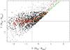 |
Fig. 4 TFR residuals (Y = MTF − Mkin) against the normalized distance modulus (X) for the calibration sample. Small open circles represent the entire sample galaxies, and larger open circles show the average values of Y in 0.1 mag. step. Black filled circles are galaxies kept after the removal of outliers in the TFR plot. Larger filled circles with error bars show the average values for them. The vertical dashed line at X = −0.5 indicates the upper limit of “bias-free” region. The thick green line shows the analytical curve giving the expected ⟨ Y ⟩ computed from the dispersion of our IRTFR. See text for details. |
The parameters needed for the calibration are the H-band magnitude mH, the maximum rotational velocity Vm, and the distance D for each sample galaxy. Our calibration sample is an all-sky sample of edge-on galaxies with uniform H-band photometry and accurate maximum rotational velocities. We use the 2MASS XSC for mH and HyperLEDA (Paturel et al. 2003a) for Vm and recession velocities. We put the following conditions on galaxies to be selected for the calibration sample.
-
1.
Their recession velocities Vr are lower than 8000 km s-1, allowing accurate correction for infall in nearby clusters.
-
2.
In order to obtain an accurate distance from Vr, we only keep galaxies having uncertainties on Vr less than 100 km s-1. Moreover, we reject all the nearby galaxies having Vr < 1000 km s-1; indeed, they are generally members of groups, and the internal motions in groups, about 80 km s-1 on the line-of-sight, introduce an additional scatter on their distances derived from the redshifts. For the same reason, we eliminate all the galaxies located within the two important clusters of galaxies having Vr < 6000 km s-1, namely all the 45 galaxies at less than 15° and 3° from the centers of the Virgo and Coma clusters, respectively.
-
3.
The uncertainties on Vm are lower than 20 km s-1; indeed, due to the high value of the slope of the IRTFR, those uncertainties are the main source of the observational dispersion of the IRTFR. Thanks to this condition, the dispersion on the IRTFR due to the measurement uncertainties is only 0.14 mag. in absolute magnitude, negligible compared to the intrinsic one (~0.3 mag, see Sect. 3.2).
-
4.
Similar to the LV galaxies, axial ratios are lower than 0.714, and the morphological types are between 3(Sb) and 8(Sdm).
-
5.
H-band magnitudes are taken from the 2MASS XSC. We use 20 mag/sq′′ isophotal elliptical aperture magnitudes (h_m_i20e) as we did for the LV galaxies. H-band apparent magnitudes were corrected for inclination and internal extinction, as well for extinction by our Galaxy. For internal extinction correction, we first derived the amount of extinction in I-band following Tully et al. (1998):
 (5)where
  is the line width at 20% corrected for inclination in km s-1 and r is the axis ratio. AI was converted to H-band extinction by AH = 0.5 AI (Sakai et al. 2000). Amount of galactic extinction toward the direction of each sample galaxy was estimated using the extinction map by Schlegel et al. (1998), and AH/E(B − V) = 0.58 was assumed.
 -
6.
In order to correct the IRTFR for the Malmquist bias, we need our sample to be complete in mH (Theureau et al. 2007). We determine the completeness limit ml by plotting log [N(≤ mH)] versus mH, where N(≤ mH) is the number of sample galaxies with an H-band magnitude lower than mH. For an homogeneous distribution of galaxies, whatever the luminosity function, the completeness to ml is equivalent to the fact that log [N(≤ mH)] follows the linear relation:
![Mathematical equation: \begin{equation} \log [N({\leq} m_H)] = 0.6\, m_H + C, \label{eq_logN} \end{equation}](/articles/aa/full_html/2011/07/aa16687-11/aa16687-11-eq249.png) (6)for any mH ≤ mlim, C being a constant. (For mH > mlim, log [N(≤ mH)] increases more slowly than this linear relation.) For our sample, we obtain mlim = 11.0.
(6)for any mH ≤ mlim, C being a constant. (For mH > mlim, log [N(≤ mH)] increases more slowly than this linear relation.) For our sample, we obtain mlim = 11.0.
Thus our final sample comprises all the galaxies figuring both in 2MASS and HyperLEDA and satisfying the conditions 1 to 6. The number of galaxies in the sample is 1463.
3.2. The unbiased IRTFR
Now we proceed to the determination of the unbiased IRTFR, following the iterative method devised by Theureau et al. (2007). At each iteration, we compute a new IRTFR; the determination of the IRTFR requires the computation of the absolute H-band magnitudes of the galaxies, which is carried out from their redshifts, corrected for non-Hubble motions in the same way as those of the galaxies of the LV sample (see Sect. 4.1).
In a first step, we determine the IRTFR from our entire calibration sample, limited however to MH ≤ −22.1. That cut is made since we found that the slope of the IRTFR changes at this value, being steeper at MH > −22.1. Moreover, all the LV galaxies with mH ≤ 11.0 are in that part of the IRTFR, for which the cut does not introduce any classical Malmquist bias. The bulk of the calibration galaxies (94%) remains in the sample after this cut. We obtain the best-fit coefficients for the IRTFR:  (7)with Vm in km s-1.
This relation is biased since the sample is not complete in a definite interval of absolute magnitudes, but only in apparent magnitudes. For a given sample galaxy, one can determine MTF from Eq. (7), and also its kinematical absolute H-band magnitude Mkin from the corrected redshift. The quantity Y = MTF − Mkin exhibits the Malmquist bias, through the uncertainties and the intrinsic dispersion of the IRTFR, since ⟨ Y ⟩ > 0 for our sample (Fig. 4).
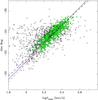 |
Fig. 5 TFR for the calibration sample. Open circles represent the entire calibration sample galaxies, and filled circles are for the “bias-free” subsample, after removal of outliers in the TFR. The dashed line is the best-fit for the entire sample (Eq. (7)), and the solid line is the best-fit result of the first iteration on the unbiased subsample (Eq. (8)). The dotted line is the result of the second iteration, which is not significantly different from the result of the first iteration. The dot-dashed line displays the TFR by Masters et al. (2008) after conversions in HI line widths and H-band magnitude systems (Eq. (9)). |
On the other hand, Teerikorpi (1975) has shown that the Malmquist bias depends only on the normalized distance modulus  , where
  is the H-band absolute magnitude of the galaxy considered as derived from the unbiased IRTFR, and Mlim the H-band absolute magnitude cut off corresponding to the limiting apparent magnitude mlim. We compute Mlim using the corrected redshift of the galaxy; for , we take the value of MTF obtained from the biased IRTFR (Eq. (7)) as a first approximation.
The plot Y(X) is shown in Fig. 4; the absence of bias for a given value of X is characterized by ⟨ Y(X) ⟩ = 0. One can see that in our sample there is a region free of bias, at X ≤ −0.5; for X > −0.5 the bias increases monotonically, reaching about 1 at X = 1. Thus, in the second iterative step, we keep only the calibration galaxies having X ≤ −0.5, in the region free of bias, and with those 584 galaxies we obtain  (8)as a new IRTFR1.
In Fig. 5 we show this fit as a solid line over the TFR distribution of the calibration sample. However, this IRTFR may not be completely bias free, since the X used was not equal to  , but to MTF − Mlim. So, in a third iterative step, we draw the new plot (X, Y) and select the galaxies in the corresponding region bias-free to compute the next IRTFR. We find that the IRTFR does not change significantly. Thus the unbiased adopted IRTFR is given by Eq. (8). The corresponding average dispersion of MTF(Vm) around the relation is σ = 0.31. In Fig. 4 the data points and average values for the sample galaxies after the removal of outliers in the TFR plot are shown as filled circles. Also in Fig. 4 the analytic function of ⟨ Y(X) ⟩ described by Theureau et al. (2007) is plotted for this sample, and it agrees very well with the data.
Note that Masters et al. (2008) have derived an IRTFR in the H-band from a sample of 2MASS calibration galaxies carefully chosen, having total extrapolated H-band magnitudes MHtot and accurate HI profile widths W50 at 50% of the peak intensity. After corrections for various statistical biases, they obtain the IRTFR in H-band as MHtot versus the width  corrected for inclination. Accounting for the relation between W50 and W20 (Paturel et al. 2003b) and the average difference MHtot − MHiso = −0.15 between total H-band magnitudes and our isophotal ones, their relation becomes
  (9)This relation leads to MH larger than ours by 0.08 ± 0.05 mag in the range 2.2 ≤ log Vm ≤ 2.5 corresponding to our LV galaxies of interest having mH ≤ 11.0. Thus the agreement is excellent, as that of the scatter of the MTF at a given Vm, which is 0.37 in Masters et al. (2008) compared to our value of 0.31.
4. Non-Hubble residual peculiar velocities of the LV sample galaxies
The non-Hubble residual peculiar velocity Vp of a galaxy is defined by  (10)where H0 is the Hubble constant, D the distance of the galaxy computed here from the IRTFR (thus independently of the redshift) and Vcorr is the measured radial velocity of the object referred to the centroid of the Local Group (LG) and corrected for the known local non-Hubble motions which include different velocities for the LG and the galaxy considered. We will use the IRTFR in Eq. (8). H0D does not depend on the value of H0 adopted if H0 is the same as the one used for the determination of the IRTFR (in this case 70 km s-1 Mpc-1).
4.1. Computation of Vcorr
To obtain Vcorr, first we convert the measured heliocentric radial velocities Vh to radial velocities VLG referred to the centroid of the LG using the equation of Tully et al. (2008):  (11)Then the known local non-Hubble motions we have to correct VLG for are the following:
(1): The repulsion of the LG from the center of the LV, recentlyevidenced convincingly by Tullyet al. (2008) thanks to veryaccurate distance measurements of galaxies located at lessthan 10 Mpcfrom us, based on the measurements of apparentbrightness of TRGB stars. The repulsion velocityof the structure at the boundary of the LV (namedthe “Local Sheet”, which includes the LG) isreported to be259 km s-1 toward ℓ = 210°, b = −2°. We are looking at a similar repulsion for our sample galaxies. Those objects and the LG are located nearly at opposite borders of the LV, and we need to correct the radial velocity of sample galaxies for this LG motion against the LV. By including the motion of the centroid of the LG within the Local Sheet (66 km s-1 towards ℓ = 11°, b = 22°; Tully et al. 2008)2, one finds that the centroid of the LG has a velocity of 202 km s-1 toward ℓ = 215°, b = 5° with respect to the LV. This results in corrections of ~− 180 km s-1 for radial velocities of our sample galaxies.
(2): The infalls towards three nearby mass concentrations, namely the Virgo cluster, the Great Attractor (GA) and the Shapley supercluster. Such corrections are necessary since the infall velocities are quite different for the sample galaxies and for the LG. The infall corrections have been carried out following Mould et al. (2000). In brief, those authors use a simple multi-attractor model; they assume the flows to be independent, thus the respective velocity infalls add to each other. The infall velocity Vf towards each attractor at the level of the LG is known. If one assumes that the attractor has the spherical symmetry with a density profile ρ(r) ∝ r−γ, then the infall velocity V(r) is: V(r) ∝ r1−γ, and one can compute the projected velocity component Vinf on the line-of-sight of the galaxy oriented towards the galaxy, of the infall velocity of the object caused by the attractor, as seen from the infalling LG, namely,  (12)where θ is the angle between the directions of the galaxy and of the attractor as seen from us, r0 is the distance of the object, ra is the distance of the attractor, and r0a is the distance between the galaxy and the attractor:
  .
.
Coordinates of the attractors and Vf values are taken from Mould et al. (2000); we have adopted for ra: 17.4 Mpc, 65.8 Mpc and 190.3 Mpc for Virgo, GA and Shapley supercluster, respectively, corresponding to H0 = 70 km s-1 Mpc-1 for velocities of the attractors corrected for infalls. The distances r0 of the LV galaxies have been computed from their redshifts referred to the centroid of the LG.
The values of Vinf for our galaxies are on the order of 50 km s-1 Mpc-1, 200 km s-1 Mpc-1, and 20 km s-1 Mpc-1 for Virgo, GA, and Shapley infalls, respectively. Taking the repulsion of the LG from the center of the LV into account, the total corrections to VLG, δVLG = δVLV − Vinf are in fact quite small, about a few tens of km s-1. If the infall corrections for these nearby mass concentrations are not applied, the peculiar velocities for most of the galaxies in the final sample are ~100−300 km s-1 smaller than when using these corrections. Those velocities are near the expected LV expansion, thus infall corrections have to be applied here.
The corrected velocities are given in Table 4.
Distances and peculiar velocities for the “unbiased” Local void sample galaxies.
4.2. Distances of the LV galaxies
We compute the distances of the LV galaxies using the IRTFR corrected for Malmquist bias (determined in Sect. 3.2). In order not to introduce any other bias, we have to treat our LV sample exactly as the calibration sample, in particular to limit it to mH ≤ 11.0 and MH ≤ −22.1, and also compute Vm the same way. Only 15 galaxies among the 36 of our LV sample have mH ≤ 11.0, and it happens that all those 15 are in the part log Vm ≥ 2.10, which corresponds to MH ≤ −22.1.
4.2.1. Determination of the maximum rotational velocity Vm
The HyperLEDA extragalactic database provides the maximum rotational velocity Vm for a number of galaxies. We have used these Vm values for those eight galaxies in our LV sample for which we took HyperLEDA 21-cm data. For the other LV galaxies, Vm was determined using the tight correlation between Vm and obtained from the calibration galaxies, namely,  (13)where is obtained from the HI profile width at 20% of the peak value corrected for resolution by
  (14)where i is the inclination of the galaxy and z the redshift. Taking the apparent axis values obtained with super-coadded image in 2MASS using J, H and K-bands, we derive i from the apparent axis ratio r by
  (15)where r0 is the intrinsic minor to major axis ratio for spiral galaxies. Following many previous studies on TFR (e.g., Tully & Fisher 1977; Sakai et al. 2000; Masters et al. 2008), we take r0 = 0.2.
4.2.2. Computation of the distances and correction for Malmquist bias
The distance modulus μ of any galaxy of our LV sample is given by  (16)where
  and
and  are the apparent and absolute H-band magnitudes corrected for galactic and internal extinction, respectively. In Table 4 we show the distances for the 15 galaxies with mH < 11.0. The photometric data are either from our own observations or from 2MASS XSC when our data are not available, as shown in Table 3. We also show the case where only 2MASS XSC photometry is used. Using only 2MASS photometry eliminates a possibility of systematic difference between data based on different facilities, but since the LV is located at low Galactic latitudes, the 2MASS photometry would suffer from contamination by foreground stars. In our own photometry we carefully removed foreground stars (Sect. 2.4), so this effect should be alleviated.
As explained above (Sect. 3.2), is determined from the value of the absolute magnitude MTF(Vm) given by the IRTFR free of Malmquist bias. However, there is a bias in the LV sample since it is limited in apparent magnitude. For a given Vm, the less luminous galaxies are not included in the sample, and this causes the average absolute magnitude ⟨ M ⟩ at Vm to be biased toward being more luminous than the true value. This effect is shown in Fig. 4 for the case of the calibration sample. In this figure, X is a normalized distance modulus MTF − Mlim where Mlim = mlim − μkin is an absolute magnitude cut off, μkin the distance modulus computed from the radial velocity, and Y a normalized magnitude MTF − Mkin, where Mkin is the absolute magnitude corresponding to mH: Mkin = mH − μkin. As discussed in Sect. 3.2, there is a bias in ⟨ Y ⟩ at X > −0.5, and thus in order to use galaxies with X > −0.5 to derive the average peculiar velocity, we need to correct the bias by applying the correction to the absolute magnitude obtained from IRTFR:  . The value of ⟨ Y(X) ⟩ is computed analytically from the TF dispersion, following Theureau et al. (2007).
Among the 15 galaxies with mH ≤ 11.0, there are six galaxies with X > −0.5. Correction factors for the distances are less than 8%, except for UGC 11426 where it is 26%.
4.3. Residual peculiar velocities of the LV galaxies
We compute the residual peculiar velocities Vp with Eq. (10), using the distance D determined in the previous section. “Bias-corrected” distances are used for the galaxies with X > −0.5. The calculated Vp are shown in Table 4. In the results based on UH88/IRSF/2MASS photometry, 10 galaxies have negative values of Vp, five have positive ones. In Fig. 6 we show the distribution of Vp against the radial velocities Vcorr. There appears to be no significant correlation between the radial velocities and the peculiar velocities.
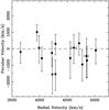 |
Fig. 6 Corrected radial velocities and peculiar velocities of the “unbiased” Local Void sample galaxies. For galaxies with the normalized distance modulus X = MTF − Mlim > −0.5, the bias corrections were applied (see text for details). |
Accounting for the uncertainties on each Vp as listed in Table 4, we obtain the average value of Vp: ⟨ Vp ⟩ is −419 + 208−251 km s-1 for the case with UH88/IRSF/2MASS photometry, and ⟨ Vp ⟩ is −319 + 204−246 km s-1 for the case with 2MASS XSC photometry alone. Thus ⟨ Vp ⟩ is not significantly different from a zero value. The values within a 3σ error range from −1172 km s-1 to 205 km s-1 for UH88/IRSF/2MASS photometry. If the LV has a general expansion, one may think that the expansion at the far boundary of the LV we investigate is comparable to that of the Local Sheet, i.e., 259 km s-1 (Tully et al. 2008), and it is slightly out of but very close to the 3σ error range of our results. Due to the size of the error, we cannot evidence such an expansion of the far-side boundary of the LV. The size of the errors in our peculiar velocities comes mainly from the intrinsic scatter of the IRTFR (σ = 0.31 in absolute magnitude). There are some other sources, such as the uncertainties on the widths of the HI line profiles, uncertainty in H-band photometry, and in radial velocities, but they are less than the effect of the scatter of the TFR.
One can note that the dispersion of the Vp around their average is also about 200 km s-1, as for the expected uncertainty, which shows that there is no systematic variations in Vp among our sample galaxies.
5. Summary and conclusions
The LV, the nearest void of galaxy distribution from us, is expected to undergo a general expansion, as in any void of galaxies, due to the lack of matter within it. Tully et al. (2008) show that the Local Group and galaxies near the Local Group, i.e., the Local Sheet at the edge of the LV, move away from the center of the LV with a velocity of 259 km s-1.
In the present study, we investigated the peculiar velocities of the galaxies located at the opposite edge of the LV with respect to the Local Group to see if they show an expansion from the center of the LV, by using the IR Tully-Fisher relation to compute their distances. The sample galaxies have an edge-on spiral morphology and radial velocities between 3000 km s-1 and 5000 km s-1. Gathering 19 HI line width measurements by ourselves and those in the literature leads to a final number of sample galaxies of 36. We also made H-band photometry for the majority of the sample galaxies. To derive the IR Tully-Fisher relation, we used a large sample of galaxies having maximum rotational velocities in HyperLEDA (Paturel et al. 2003a) and H-band isophotal magnitudes in 2MASS XSC, complete to mH = 11.0. The IRTFR free from the Malmquist bias was obtained from that sample, and then was used to compute the distances of the 15 LV galaxies having mH ≤ 11.0. After the corrections for the infall motions toward the nearby clusters/concentrations and the motion of the Local Group away from the center of the LV, the residual peculiar velocities Vp for the 15 LV galaxies have been obtained. The average value after the correction for the Malmquist bias (which is thought to affect Vp of some of the sample galaxies) is  km s-1. This is not significantly different from zero, and it does not reject the possibility that these galaxies have a motion against the LV equivalent to that of the Local Sheet (259 km s-1).
Padilla et al. (2005) made a Λ CDM numerical simulation on the properties of dark matter halos and galaxies around voids and find a linear relation between the maximum outflow velocity vmax and the distance from the center of the void rvoid: vmax = v0rvoid, where the best-fit value of v0 is 14.5 km s-1 h Mpc-1. If we adopt the radius of the void to be 2500 km s-1 and h = 0.7, this gives the vmax of 360 km s-1. Such a value is significantly higher than the motion of 259 ± 25 km s-1 of the Local Sheet away from the LV, and at 3.7σ from our  . Thus it does not seem
to account correctly for the expansion of the LV. However, the geometry of the LV is more complex than a simple sphere, consisting in a void within two large voids (Tully et al. 2008). Thus the maximum velocity Padilla et al. (2005) measured in their simulated voids might not be fully appropriate for the comparison with the expansion velocity of the LV.
Finally, the uncertainty ~200 km s-1 of our is not sufficient for proving the expansion found by Tully et al. (2008) for the Local Sheet. Smaller uncertainty would be achieved if we were able to use more galaxies – i.e., using galaxies with apparent magnitude fainter than mH = 11.0. However, since the number of galaxies at the far-side of the LV, which can be used for IRTFR, would not exceed ~50, we may need an alternative, more accurate distance estimator to conclusively know whether the opposite edge of the LV undergoes an expansion.
Note that Eq. (8) can be written as MTF = −8.58log Vm−4.06 + 5log (H0/70) if we take a different value for H0.
There is an error in the calculation of the galactic longitude of this motion in Tully et al. (2008) (i.e., ℓ of  ) in their Table 3.
Acknowledgments
We thank staff members of the telescope facilities used in this work (Okayama Astrophysical Observatory, Nançay radiotelescope, the Infrared Survey Facility, and the University of Hawaii 2.2 m telescope) for their support during observations. We would like to thank the referee (B. Tully) for helpful comments that improved the paper. II is grateful to M. Saitō who raised the initial idea of this work, A. T. Roman for his participation in the observations in Okayama, and K. Nakanishi and K. Ohta for supporting observations and giving thoughtful suggestions. II was supported by a Research Fellowship of the Japan Society for the Promotion of Science (JSPS) for Young Scientists during parts of this research.
References
- Bottinelli, L., Gouguenheim, L., Fouqué, P., & Paturel, G. 1990, A&AS, 82, 391 [NASA ADS] [Google Scholar]
- Burstein, D. 2000, in Cosmic Flows Workshop, ed. S. Courteau, & J. Willick, ASP Conf. Ser., 201, 178 [Google Scholar]
- Ceccarelli, L., Padilla, N. D., Valotto, C., & Lambas, D. G. 2006, MNRAS, 373, 1440 [NASA ADS] [CrossRef] [Google Scholar]
- Faber, S. M., & Burstein, D. 1988, Motions of galaxies in the neighborhood of the local group, ed. V. C. Rubin, & G. V Coyne, 115 [Google Scholar]
- Fouqué, P., Durand, N., Bottinelli, L., Gouguenheim, L., & Paturel, G. 1990, A&AS, 86, 473 [NASA ADS] [Google Scholar]
- Hewitt, J. N., Haynes, M. P., & Giovanelli, R. 1983, AJ, 88, 272 [NASA ADS] [CrossRef] [Google Scholar]
- Masters, K. L., Springob, C. M., & Huchra, J. P. 2008, AJ, 135, 1738 [NASA ADS] [CrossRef] [Google Scholar]
- Mould, J. R., Huchra, J. P., Freedman, W. L., et al. 2000, ApJ, 529, 786 [NASA ADS] [CrossRef] [Google Scholar]
- Nagashima, C., Nagayama, T., Nakajima, Y., et al. 1999, in Star Formation 1999, Proc. Star Formation 1999, held in Nagoya, Japan, June 21−25, ed. T. Nakamoto, Nobeyama Radio Observatory, 397 [Google Scholar]
- Nagayama, T., Nagashima, C., Nakajima, Y., et al. 2003, in Instrument Design and Performance for Optical/Infrared Ground-based Telescopes, ed. M. Iye, & A. F. M. Moorwood, Proc. SPIE, 4841, 459 [Google Scholar]
- Nakanishi, K., Takata, T., Yamada, T., et al. 1997, ApJS, 112, 245 [NASA ADS] [CrossRef] [Google Scholar]
- Nilson, P. 1973, Uppsala general catalogue of galaxies, ed. P. Nilson, Uppsala Astronomiska Observatoriums Annaler [Google Scholar]
- Padilla, N. D., Ceccarelli, L., & Lambas, D. G. 2005, MNRAS, 363, 977 [NASA ADS] [CrossRef] [Google Scholar]
- Paturel, G., Petit, C., Prugniel, P., et al. 2003a, A&A, 412, 45 [NASA ADS] [CrossRef] [EDP Sciences] [Google Scholar]
- Paturel, G., Theureau, G., Bottinelli, L., et al. 2003b, A&A, 412, 57 [NASA ADS] [CrossRef] [EDP Sciences] [Google Scholar]
- Roman, A. T., Iwata, I., & Saitō, M. 2000, ApJS, 127, 27 [NASA ADS] [CrossRef] [Google Scholar]
- Sakai, S., Mould, J. R., Hughes, S. M. G., et al. 2000, ApJ, 529, 698 [NASA ADS] [CrossRef] [Google Scholar]
- Saunders, W., Sutherland, W. J., Maddox, S. J., et al. 2000, MNRAS, 317, 55 [NASA ADS] [CrossRef] [Google Scholar]
- Schlegel, D. J., Finkbeiner, D. P., & Davis, M. 1998, ApJ, 500, 525 [NASA ADS] [CrossRef] [Google Scholar]
- Sheth, R. K., & van de Weygaert, R. 2004, MNRAS, 350, 517 [NASA ADS] [CrossRef] [Google Scholar]
- Skrutskie, M. F., Cutri, R. M., Stiening, R., et al. 2006, AJ, 131, 1163 [NASA ADS] [CrossRef] [Google Scholar]
- Springob, C. M., Haynes, M. P., Giovanelli, R., & Kent, B. R. 2005, ApJS, 160, 149 [Google Scholar]
- Teerikorpi, P. 1975, A&A, 45, 117 [NASA ADS] [Google Scholar]
- Theureau, G., Hanski, M. O., Coudreau, N., Hallet, N., & Martin, J.-M. 2007, A&A, 465, 71 [NASA ADS] [CrossRef] [EDP Sciences] [Google Scholar]
- Tully, R. B., & Fisher, J. R. 1977, A&A, 54, 661 [NASA ADS] [Google Scholar]
- Tully, R. B., & Fisher, J. R. 1987, Nearby Galaxies Atlas, ed. R. B. Tully, & J. R. Fisher (Cambridge University Press) [Google Scholar]
- Tully, R. B., Pierce, M. J., Huang, J., et al. 1998, AJ, 115, 2264 [NASA ADS] [CrossRef] [Google Scholar]
- Tully, R. B., Shaya, E. J., Karachentsev, I. D., et al. 2008, ApJ, 676, 184 [NASA ADS] [CrossRef] [Google Scholar]
All Tables
List of galaxies with new heliocentric radial velocity Vh measurements in km s-1 in the catalog of Roman et al. (2000).
Summary of the results of our HI 21 cm line observations with the Nançay radiotelescope.
Summary of the near-infrared photometry and corrected HI line widths for the final Local Void sample galaxies.
All Figures
|
Fig. 1 Spatial distribution of the Local Void sample galaxies in galactic coordinates. Small filled circles represent galaxies in the IRAS PSCz catalog (Saunders et al. 2000) with radial velocity between 3000 km s-1 and 5000 km s-1. Larger circles are the Local Void sample galaxies in this study (50 galaxies, see Sect. 2.1). Filled circles are for the 36 galaxies included in the final sample (see Sect. 2.3), while open circles are those not in the final sample. Dashed lines indicate latitudes in the supergalactic coordinates, and the cross shows the position of the North supergalactic pole. The position opposite to the Local Velocity Anomaly defined by Burstein (2000) is indicated by a blue asterisk. |
| In the text | |
|
Fig. 2 Distribution of the Local Void sample galaxies in the galactic longitude – radial velocity planes. a)−c) display the galaxies with galactic latitude −30° < b < 0°, 0° < b < 20° and 20° < b < 40°, respectively. The meaning of symbols are the same as in Fig. 1: filled circles represent galaxies in the IRAS PSCz catalog (Saunders et al. 2000) with radial velocities. Larger circles are the 50 Local Void sample galaxies in this study. Larger filled circles are for the 36 galaxies included in the final sample, and open circles are those not in the final sample. |
| In the text | |
|
Fig. 3 The HI 21 cm line profiles of the 30 Local Void galaxies detected with Nançay radiotelescope and of the possibly detected one (UGC 11198). The horizontal axis is the radial velocity in km s-1 and the vertical axis is the flux density in mJy. The hanning and boxcar smoothing are applied and the subtraction of the polynomial fitted baseline is made. |
| In the text | |
|
Fig. 4 TFR residuals (Y = MTF − Mkin) against the normalized distance modulus (X) for the calibration sample. Small open circles represent the entire sample galaxies, and larger open circles show the average values of Y in 0.1 mag. step. Black filled circles are galaxies kept after the removal of outliers in the TFR plot. Larger filled circles with error bars show the average values for them. The vertical dashed line at X = −0.5 indicates the upper limit of “bias-free” region. The thick green line shows the analytical curve giving the expected ⟨ Y ⟩ computed from the dispersion of our IRTFR. See text for details. |
| In the text | |
|
Fig. 5 TFR for the calibration sample. Open circles represent the entire calibration sample galaxies, and filled circles are for the “bias-free” subsample, after removal of outliers in the TFR. The dashed line is the best-fit for the entire sample (Eq. (7)), and the solid line is the best-fit result of the first iteration on the unbiased subsample (Eq. (8)). The dotted line is the result of the second iteration, which is not significantly different from the result of the first iteration. The dot-dashed line displays the TFR by Masters et al. (2008) after conversions in HI line widths and H-band magnitude systems (Eq. (9)). |
| In the text | |
|
Fig. 6 Corrected radial velocities and peculiar velocities of the “unbiased” Local Void sample galaxies. For galaxies with the normalized distance modulus X = MTF − Mlim > −0.5, the bias corrections were applied (see text for details). |
| In the text | |
Current usage metrics show cumulative count of Article Views (full-text article views including HTML views, PDF and ePub downloads, according to the available data) and Abstracts Views on Vision4Press platform.
Data correspond to usage on the plateform after 2015. The current usage metrics is available 48-96 hours after online publication and is updated daily on week days.
Initial download of the metrics may take a while.