| Issue |
A&A
Volume 531, July 2011
|
|
|---|---|---|
| Article Number | A167 | |
| Number of page(s) | 10 | |
| Section | The Sun | |
| DOI | https://doi.org/10.1051/0004-6361/201116536 | |
| Published online | 08 July 2011 | |
Kink oscillations of flowing threads in solar prominences
1
Centre for Plasma Astrophysics, Department of MathematicsKatholieke Universiteit Leuven, Celestijnenlaan 200B, 3001 Leuven, Belgium
e-mail: roberto.soler@wis.kuleuven.be
2
Solar Physics Group, Departament de Física, Universitat de les Illes Balears, 07122 Palma de Mallorca, Spain
Received: 18 January 2011
Accepted: 16 June 2011
Context. Recent observations by Hinode/SOT show that MHD waves and mass flows are simultaneously present in the fine structure of solar prominences.
Aims. We investigate standing kink magnetohydrodynamic (MHD) waves in flowing prominence threads from a theoretical point of view. We model a prominence fine structure as a cylindrical magnetic tube embedded in the solar corona with its ends line-tied in the photosphere. The magnetic cylinder is composed of a region with dense prominence plasma, which is flowing along the magnetic tube, whereas the rest of the flux tube is occupied by coronal plasma.
Methods. We use the WKB approximation to obtain analytical expressions for the period and the amplitude of the fundamental mode as functions of the flow velocity. In addition, we solve the full problem numerically by means of time-dependent simulations.
Results. We find that both the period and the amplitude of the standing MHD waves vary in time as the prominence thread flows along the magnetic structure. The fundamental kink mode is a good description for the time-dependent evolution of the oscillations, and the analytical expressions in the WKB approximation are in agreement with the full numerical results.
Conclusions. The presence of flow modifies the period of the oscillations with respect to the static case. However, for realistic flow velocities this effect might fall within the error bars of the observations. The variation of the amplitude due to the flow leads to apparent damping or amplification of the oscillations, which could modify the real rate of attenuation caused by an additional damping mechanism.
Key words: Sun: filaments, prominences / Sun: oscillations / Sun: corona / magnetohydrodynamics (MHD) / waves
© ESO, 2011
1. Introduction
Recent observational evidence of ubiquitous periodically varying features in the solar corona (e.g., Tomczyk et al. 2007; Jess et al. 2009; Tomczyk & McIntosh 2009; Wang et al. 2009) has raised the debate on whether these observations are caused by magnetohydrodynamic (MHD) waves or by quasi-periodic flows (see, e.g., De Pontieu & McIntosh 2010). There seem to be strong theoretical arguments supporting the wave interpretation (e.g., Erdélyi & Fedun 2007; Van Doorsselaere et al. 2008; Terradas et al. 2010; Verth et al. 2010). However, waves and flows are not mutually exclusive and, in fact, both phenomena have been simultaneously observed in the fine structure of solar prominences (e.g., Okamoto et al. 2007). This offers us the opportunity to study the interaction between waves and flows in the solar atmosphere.
The fine structure of solar prominences is clearly visible in the high-resolution Hα and Ca II H-line images from the Solar Optical Telescope (SOT) aboard the Hinode satellite (e.g., Okamoto et al. 2007; Berger et al. 2008; Chae et al. 2008; Ning et al. 2009; Schmieder et al. 2010; Chae 2010). When observed above the limb, vertical structures are commonly seen in quiescent prominences (e.g., Berger et al. 2008; Chae et al. 2008; Chae 2010), while horizontal threadlike structures are usually observed in active region prominences (e.g., Okamoto et al. 2007). Although it is apparently difficult to reconcile both pictures, some authors (e.g., Schmieder et al. 2010) have suggested that vertical threads might actually be a pile up of horizontal threads which appear as vertical structures when projected on the plane of the sky. This idea is consistent with Hα observations of filaments on the solar disk from the Swedish Solar Telescope (e.g., Lin et al. 2008, 2009), in which the filament fine structure is seen as thin and long dark ribbons. On the other hand, other authors (e.g., Chae 2010) have argued that vertical threads are real and are an indication of the existence of vertical magnetic fields in quiescent prominences. Thus, it remains unclear whether all prominences have the same magnetic structure or, on the contrary, the magnetic field in quiescent prominences is predominantly vertical and active region prominences have horizontal fields. A recent review on the properties of prominence threads can be found in Lin (2010).
There are many evidences of transverse oscillations of the fine structures of both active region and quiescent prominences, which have been interpreted in terms of kink MHD waves (see the recent reviews by Ballester 2006; Oliver 2009; Arregui & Ballester 2010). The reported periods are usually in a narrow band between 2 and 10 minutes, while the oscillations are typically damped after a few periods. In addition, flows and mass motions in prominences have been also reported (e.g., Zirker et al. 1998; Wang 1999; Kucera et al. 2003; Lin et al. 2003; Ahn et al. 2010). The typical flow velocities are less than 30 km s-1 in quiescent prominences, although larger values up to 40–50 km s-1 have been observed in active region prominences.
The work of Okamoto et al. (2007) is an example of simultaneous transverse oscillations and mass flows in prominence fine structures observed with Hinode/SOT. In the present paper we focus on the theoretical analysis of the event reported by Okamoto et al. (2007). Similar observations of simultaneous flows and oscillations have been reported by Ofman & Wang (2008) in coronal loops and by Cao et al. (2010) in filament footpoints. Also, the recent work by Antolin & Verwichte (2011) on observations of transverse oscillations of loops with coronal rain is relevant for our present theoretical investigation. Okamoto et al. (2007) observed an active region prominence formed by a myriad of horizontal magnetic flux tubes which are partially outlined by threads of cool and dense prominence plasma. The magnetic tubes are probably rooted in the solar photosphere. Although only the part of the tubes filled with prominence material can be seen in the Ca II H-line images, the length of the whole magnetic tube must be much longer than the length of the prominence threads, which is roughly between 3000 km and 16 000 km. Okamoto et al. (2007) detected that some threads were flowing along the magnetic tubes and simultaneously oscillating in the vertical direction. The mean period of the oscillations was 3 min and the apparent flow velocity on the plane of sky was around 40 km s-1. The oscillations were in phase along the whole length of the threads, and the wavelength was estimated to be at least 250 000 km.
The event observed by Okamoto et al. (2007) was studied from a theoretical point of view by Terradas et al. (2008), who interpreted the observations in terms of standing kink MHD modes supported by the magnetic structure (see, e.g., Edwin & Roberts 1983; Díaz et al. 2002; Goossens et al. 2009; Soler et al. 2010). An interpretation of the observations by Okamoto et al. (2007) in terms of kink modes was also suggested by Erdélyi & Fedun (2007) and Van Doorsselaere et al. (2008). Terradas et al. (2008) used the observed wave properties provided by Okamoto et al. (2007) to perform a seismological estimation of a lower bound of the prominence Alfvén speed. The time-dependent numerical simulations by Terradas et al. (2008) suggested that the influence of the flow on the period was small. Nevertheless, the precise effect of the flow was not assessed in their work because a detailed parametric study was not performed. The purpose of this paper is to advance the analysis of the event observed by Okamoto et al. (2007) by combining both analytical and numerical methods. In the analytical part, we use the WKB approximation to assess the effect of the flow on the period and the amplitude of the transverse oscillations. Expressions of these quantities as functions of the relevant parameters of the model are obtained. In the numerical part, we go beyond the WKB approximation and solve the full time-dependent problem. The implications of our results for the magneto-seismology of prominences are also discussed.
This paper is organized as follows. Section 2 contains the model configuration and the basic governing equations. The analytical investigation of standing kink MHD waves in flowing prominence threads using the WKB approximation is included in Sect. 3, while the full numerical solution of the time-dependent problem is performed in Sect. 4. Finally, our results are discussed in Sect. 5.
2. Model and basic equations
The background model in which the waves are superimposed is schematically shown in Fig. 1. It is composed of a straight and cylindrical magnetic flux tube of radius R and length L, whose ends are fixed at two rigid walls representing line-tying at the solar photosphere. The z-axis is chosen so that it coincides with the axis of the tube, and the photospheric walls are located at z = ± L/2. The magnetic tube is partially filled with prominence plasma of density ρp, while the rest of the tube, i.e., the evacuated part, is occupied by less dense plasma of density ρe. The density of the external plasma is the density of the coronal medium, ρc. The length of the prominence region (thread) is Lp. The thread flows along the tube as a block with constant speed v0. The magnetic field is B = Bez, with B homogeneous. As the β = 0 approximation is used in the present work, with β the ratio of the gas pressure to the magnetic pressure, the plasma temperature is irrelevant for the study of kink MHD waves supported by the model. In the absence of flow, standing kink MHD waves supported by the present model were investigated by Joarder et al. (1997) and Díaz et al. (2001) in Cartesian geometry, and by Díaz et al. (2002), Dymova & Ruderman (2005), Díaz et al. (2010), and Soler et al. (2010) in cylindrical geometry.
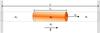 |
Fig. 1 Sketch of the prominence fine structure model adopted in this work. |
We adopt the TT approximation, which is valid for R/L ≪ 1 and R/Lp ≪ 1. To check whether or not this approximation is reasonable in the context of prominence threads, we take into account that the values of R and Lp reported by the observations (e.g., Lin 2004; Okamoto et al. 2007; Lin et al. 2008) are in the ranges 50 km ≲ R ≲ 300 km and 3000 km ≲ Lp ≲ 28 000 km, respectively, and assume L ~ 105 km as a typical length for the magnetic tube. We obtain R/Lp and R/L in the ranges 3 × 10⁻³ ≲ R/Lp ≲ 0.1 and 5 × 10⁻⁴ ≲ R/L ≲ 3 × 10⁻³, meaning that the use of the TT approximation is justified in prominence fine structures. In the case v0 = 0, the basic equation governing linear kink MHD waves of the flux tube in the TT approximation was derived by Dymova & Ruderman (2005) in their Eq. (21). In the absence of flow, the TT approximation was used by Dymova & Ruderman (2005), Díaz et al. (2010), and Soler et al. (2010). The results of these works fully agree with the general results beyond the TT approximation by Joarder et al. (1997), Díaz et al. (2001), and Díaz et al. (2002).
In the presence of flow, an intuitive generalization of Eq. (21) of Dymova & Ruderman (2005) was performed by Terradas et al. (2008) in their Eq. (2). Mathematically, Morton & Erdélyi (2010a) also considered the variation of density with time and obtained a similar expression in their Eq. (18). We refer the reader to Terradas et al. (2008) and Morton & Erdélyi (2010a) for a detailed derivation of the basic equation. In the mathematical derivation of Morton & Erdélyi (2010a) it is assumed that the difference of the flow velocity between the internal and external plasma is small, i.e., much smaller than the Alfvén velocity. So, we restrict our present investigation to values of the flow velocity that satisfy v0/vAp ≪ 1, where  is the prominence Alfvén speed. Assuming B = 50 G and ρp = 10-10 kg m-3 as realistic values of the magnetic field strength and density in active region prominences, we obtain vAp ≈ 446 km s-1. Since the flow velocities on the plane of sky estimated by Okamoto et al. (2007) are in the interval between 15 km -1 to 46 km s-1 (see their Table 1), the restriction v0/vAp ≪ 1 is satisfied for realistic parameters in prominences.
Thus, the governing equation we study in the present work is 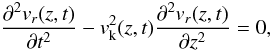 (1)which has to be solved along with the condition of line-tying at the photosphere expressed as vr(± L/2,t) = 0, and a given initial condition at t = 0. In Eq. (1), vr(z,t) is the radial velocity perturbation at the tube boundary and vk(z,t) is the kink speed, which in our model is a function of z and t, namely
 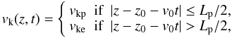 (2)where
 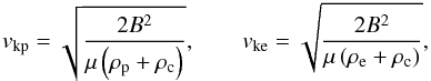 (3)with μ the magnetic permittivity, and z0 corresponds to the position of the center of the prominence thread with respect to the center of the magnetic tube at t = 0. Note that z0 < 0 if the thread is initially located on the left-hand side of the center of the tube, whereas z0 > 0 if the thread is initially located on the right-hand side. We see that the flow does not explicitly appear in Eq. (1) since it is enclosed in the definition of vk(z,t) given in Eq. (2). Terradas et al. (2008) performed time-dependent simulations and solved Eq. (1) numerically. Here, our aim is to solve Eq. (1) by using both analytical and numerical methods.
3. Analytical investigation: WKB approximation
We solve Eq. (1) analytically by using the Wentzel-Kramers-Brillouin (WKB) approximation (see, e.g., Bender & Orszag 1978, for details about the method). The WKB approximation has been recently applied to the investigation of MHD waves in cooling coronal loops (Morton et al. 2010; Morton & Erdélyi 2010a,b). In particular, the work by Morton & Erdélyi (2010a) is especially relevant for the present investigation as they studied kink oscillations of coronal loops with variable background.
The WKB approximation is an approximate method to study waves in a changing background whose properties are smooth functions of space and/or time. In the present application of the WKB approximation we assume that the time scale related to the waves, e.g., the period, is much shorter than the time scale related to the changes of the background configuration. Under these conditions, it is possible to define a time-dependent frequency which slowly varies because of the changing background. To apply the WKB approximation we define the parameter δ as  (4)The validity of the WKB approximation is restricted to small values of δ so as Pδ ≪ 1, where P is the period of the oscillations. In the observations by Okamoto et al. (2007), the mean flow velocity and period are v0 ≈ 40 km s-1 and P ≈ 3 min. For L ~ 105 km these values result Pδ ≈ 0.072, meaning that the condition of applicability of the WKB approximation is fulfilled in the case of transverse oscillations of flowing threads.
Using the parameter δ we define the dimensionless time, t1, as  (5)and we express the solution to Eq. (1) in the following form
  (6)with Q1(z,t1) and Ω1(t1) functions to be determined. Next, we combine Eqs. (1) and (6), and separate the different terms according to their order with respect to δ. As δ is small, the dominant terms are those with the lowest order in δ. We obtain two equations for Q1(z,t1) and Ω1(t1) taking the terms with
  and
and  , namely
  Equations (7) and (8) are equivalent to Eqs. (24) and (25) of Morton & Erdélyi (2010a), respectively.
Now, we define the time-dependent frequency,  , as
, as  (9)which allows us to rewrite Eq. (7) as follows
  (10)Equation (10) has to be solved taking into account the boundary conditions Q1(± L/2,t1) = 0 due to photospheric line-tying. By solving Eq. (10), the dependence on z of function Q1(z,t1) can be obtained. In addition, since
  is a piecewise constant function of z (see Eq. (2)), the analytical solutions to Eq. (10) are trigonometric functions with time-dependent arguments. Thus, the general solution to Eq. (10) satisfying the boundary conditions at z = ± L/2 is
 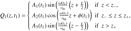 (11)where A1(t1), A2(t1), and A3(t1) are time-dependent coefficients, φ(t1) is a time-dependent phase, and z − and z + denote the locations of the interfaces between the prominence thread and the evacuated regions, namely
 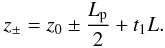 (12)The locations of the interfaces change as the dense thread moves along the magentic tube. Q1 must satisfy appropriate boundary conditions at z = z ± . Since the interfaces correspond to contact discontinuities (see Goedbloed & Poedts 2004), the boundary conditions are
 ![\begin{equation} \left[\left[Q_1 \right]\right] = 0, \quad \left[\left[ \frac{\pd Q_1 }{\pd z} \right]\right] = 0,\label{eq:boundary} \end{equation}](/articles/aa/full_html/2011/07/aa16536-11/aa16536-11-eq75.png) (13)where [ [X ] ] stands for the jump of the quantity X at z = z ± .
(13)where [ [X ] ] stands for the jump of the quantity X at z = z ± .
Applying the conditions of Eq. (13) on the solutions given by Eq. (11), we arrive at the following equation ![\begin{eqnarray} && \frac{\cke}{\ckp} \tan \left[ \frac{\omega\left( t_1 \right)}{\cke} \left( z_0 - \frac{L-\lp}{2} + t_1 L \right) \right] \nonumber \\ &=& \frac{\ckp + \cke \cot \left( \frac{\omega\left( t_1 \right)}{\ckp} \lp \right) \tan \left[ \frac{\omega\left( t_1 \right)}{\cke} \left(z_0 + \frac{L-\lp}{2} + t_1 L \right) \right] }{\ckp \cot \left( \frac{\omega\left( t_1 \right)}{\ckp} \lp \right) - \cke \tan \left[ \frac{\omega\left( t_1 \right)}{\cke} \left(z_0 + \frac{L-\lp}{2} + t_1 L \right) \right]}\cdot \label{eq:disper} \end{eqnarray}](/articles/aa/full_html/2011/07/aa16536-11/aa16536-11-eq79.png) (14)Equation (14) is the time-dependent dispersion relation. For fixed t1, the solution of Eq. (14) is . Note that, although Eq. (14) is written in a more compact form, it is consistent with dispersion relations previously obtained for normal modes in the static case, i.e., v0 = 0. Equation (14) with v0 = 0 is equivalent to Eq. (11) of Soler et al. (2010) if the substitutions
(14)Equation (14) is the time-dependent dispersion relation. For fixed t1, the solution of Eq. (14) is . Note that, although Eq. (14) is written in a more compact form, it is consistent with dispersion relations previously obtained for normal modes in the static case, i.e., v0 = 0. Equation (14) with v0 = 0 is equivalent to Eq. (11) of Soler et al. (2010) if the substitutions  and
and  are performed in their expression. Also for v0 = 0, Eq. (14) is similar to Eq. (17) of Joarder & Roberts (1992) and Eq. (A5) of Oliver et al. (1993) obtained in Cartesian geometry.
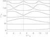 |
Fig. 2 Dimensionless frequency, ωτAp, versus time in units of the internal Alfvén travel time, τAp = L/vAp. Results corresponding to the fundamental mode and the lowest seven harmonics obtained by numerically solving Eq. (14) for a flowing thread with Lp/L = 0.1, v0/vAp = 0.05, and z0/L = −0.25. The vertical dotted line denotes the time when the prominence thread is centered within the flux tube. |
We have solved Eq. (14) by standard numerical techniques. The frequencies of the fundamental mode and of the lowest seven harmonics with respect to z are displayed as functions of time in Fig. 2 for a particular set of parameters. We find that the dispersion diagram is symmetric with the time when the thread is located at the center of the magnetic tube (denoted by a vertical dotted line in Fig. 2) as point of symmetry. The fundamental mode and the first harmonic are smooth functions of time. The other harmonics displayed in Fig. 2 show a complicated set of couplings and avoided crossings. The reason for this behavior is that the fundamental mode and the first harmonic correspond to global oscillations of the flux tube because both the prominence and the evacuated parts of the tube are disturbed. On the contrary, high harmonics correspond to modes more confined within one of these regions. Thus, the collection of modes and their properties are similar to those studied by Joarder & Roberts (1992) and Oliver et al. (1993) in slab geometry.
3.1. Approximation to the fundamental mode frequency
From hereon we restrict our analysis to the fundamental mode of oscillation, whose frequency is the lowest order solution to Eq. (14). To obtain an approximation to the frequency, we perform a Taylor expansion of Eq. (14) and neglect terms with  and higher orders in ω. The following expression is obtained
 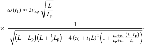 (15)The effect of the flow is contained in the denominator of the right-hand side of Eq. (15). We see that the effect of the flow on the frequency is more complicated than a simple Doppler shift. There are two reasons that cause this dependence. On the one hand, our model is a complicated structure in the sense that only the dense prominence material is moving. It is well known that a wave propagating in a uniform magnetic tube with a constant siphon flow is affected by a constant Doppler shift of the frequency due to the flow. However, the effect of the flow is not so simple in more complicated configurations. Even in the case of a flux tube with a constant flow within the tube but no flow in the exterior of the tube the wave frequencies suffer corrections due to the flow that are not simple frequency shifts (see, e.g., Nakariakov & Roberts 1995; Terra-Homem et al. 2003). Our configuration is very different from the typical uniform magnetic flux tube with a siphon flow, so that the frequency is also modified by the change of position of the dense plasma within the magnetic tube. On the other hand, we are dealing with standing modes, not propagating waves. For standing modes in flux tubes Terradas et al. (2011) have shown that flow produces a spatially dependent phase shift along the magnetic tube. In our case, this phase shift is contained in the time-dependent phase φ(t1) of Eq. (11).
For typical prominence and coronal densities, ρp ≫ ρc and ρp ≫ ρe. Therefore, the term with the ratio of densities in the denominator of Eq. (15) can be neglected. Then, Eq. (15) simplifies to  (16)In the absence of flow, i.e., t1 = 0, and for z0 = 0, Eq. (16) loses its time dependence and becomes,
  (17)Equation (17) is consistent with the approximation of the normal mode frequency obtained by Díaz et al. (2010, Eq. (8a)). For Lp ≪ L we can approximate
  , and Eq. (17) reduces to the expression found by Soler et al. (2010, Eq. (17)). Although the case Lp → L is very unrealistic in prominences because the observed lengths of prominence threads correspond to Lp/L ≪ 1, it is instructive to take into account this limit. For Lp → L the frequency given in Eq. (17) tends to infinity. The reason is that the fundamental kink mode behaves as a hybrid mode like those described by Oliver et al. (1993) in a Cartesian slab (see also the string modes investigated by Joarder & Roberts 1992). Equations (15)–(17) are approximations of the hybrid mode frequency. As explained by Oliver et al. (1993), hybrid modes owe their existence to the presence of both the dense part and the evacuated part of the tube. In the limit Lp → L the evacuated part is absent and the hybrid kink mode disappears. Thus for Lp → L the fundamental kink mode is not the hybrid mode but the first internal mode with frequency
  (18)Since Lp/L ≪ 1 in prominences, the fundamental mode in a realistic thread is the hybrid mode and Eqs. (15)–(17) apply.
We plot in Fig. 3 the solution of Eq. (14) for the fundamental mode as a function of time, along with the analytical approximation given by Eq. (16). Equation (14) has been solved by using standard numerical methods to obtain the roots of transcendental equations. These computations have been performed for different values of Lp/L and v0/vAp, and for fixed z0/L. There is a very good agreement between the full solution (solid lines in Fig. 3) and the approximation (symbols). From Fig. 3a, we see that the frequency decreases as the length of the prominence thread increases. On the other hand, Fig. 3b shows that the variation of the frequency with time is more important as the flow velocity gets faster. We find that the minimum of the frequency takes place when the thread is centered within the magnetic tube. Therefore, the minimum of the frequency depends on both the initial position of the thread and the flow velocity since the relation z0 + v0t = 0 has to be satisfied.
Equation (16) corresponds to the instantaneous frequency. However, the actual temporal dependence of the oscillation in the WKB approximation is given by function Ω1(t1). We obtain Ω1(t1) from Eq. (9) by integrating given by Eq. (16). Hence, ![\begin{eqnarray} \Omega_1(t_1) &=& \frac{\ckp}{\sqrt{L \lp}}\left\{ \arctan \left[ \frac{2 \left( z_0 + t_1 L \right)}{\sqrt{\left( L - \lp \right) \left( L + \frac{1}{3} \lp \right) - 4 \left( z_0 + t_1 L \right)^2}} \right] \right. \nonumber \\ &-& \left. \arctan \left[ \frac{2 z_0 }{\sqrt{\left( L - \lp \right) \left( L + \frac{1}{3} \lp \right) - 4 z_0^2}} \right] \right\}, \end{eqnarray}](/articles/aa/full_html/2011/07/aa16536-11/aa16536-11-eq106.png) (19)where we have used the condition Ω1 = 0 at t1 = 0.
(19)where we have used the condition Ω1 = 0 at t1 = 0.
3.2. Dependence of the amplitude on time
Here, we estimate the variation of the amplitude of the oscillations with time. To do so, we use Eq. (8). By taking into account the definition of the time-dependent frequency (Eq. (9)), we rewrite Eq. (8) as  (20)Next, we consider the approximate ω(t1) for the fundamental mode obtained in Eq. (15) to express this last equation as
  (21)Note that to solve Eq. (21) we do not have to care about the dependence of Q1 on z. For a given z, Eq. (21) can be integrated to obtain the temporal dependence of Q1 at a fixed position, namely
 ![\begin{eqnarray} Q_1 (z,t_1) &=& Q_0(z) \left[ \frac{\left( L - \lp \right) \left( L + \frac{1}{3} \lp \right) - 4 \left( z_0 + t_1 L \right)^2}{\left( L - \lp \right) \left( L + \frac{1}{3} \lp \right) - 4 z_0^2} \right]^{1/4},\label{eq:qtempdepsol} \end{eqnarray}](/articles/aa/full_html/2011/07/aa16536-11/aa16536-11-eq111.png) (22)where Q0(z) is the amplitude at t1 = 0. Thus, Eq. (11) gives the spatial dependence of Q1 for a fixed time t1, while Eq. (22) provides the temporal dependence at a fixed position z. By comparing Eqs. (16) and (22), we see that
(22)where Q0(z) is the amplitude at t1 = 0. Thus, Eq. (11) gives the spatial dependence of Q1 for a fixed time t1, while Eq. (22) provides the temporal dependence at a fixed position z. By comparing Eqs. (16) and (22), we see that  . Then, the amplitude of the oscillation decreases when the thread flows from the center of the tube to the footpoint, and increases otherwise. This means that the amplitude is maximal when the thread is located at the center of the magnetic tube.
We must bear in mind that Eq. (22) was derived from the terms with in the governing equation, whereas the leading terms when δ is a small parameter are those with  . Therefore, we have to be cautious about the actual accuracy of Eq. (22), although we expect the behavior of the amplitude with time to be, at least, qualitatively described by Eq. (22).
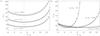 |
Fig. 3 Dimensionless frequency, ωτAp, versus time in units of the internal Alfvén travel time, τAp = L/vAp, for a) Lp/L = 0.05, 0.1, 0.2 with v0/vAp = 0.05, and b) v0/vAp = 0.03, 0.05, 0.1 with Lp/L = 0.1. In all cases, z0/L = −0.25. The solid lines are the results obtained by numerically solving Eq. (14), whereas the symbols correspond to the analytical approximation given by Eq. (16). The vertical dotted line in panel a) denotes the minimum of the curves, i.e., the time when the prominence thread is centered within the flux tube. |
3.3. Application to magneto-seismology
The analytical expression of the fundamental mode frequency found before can be used to perform magneto-seismology of prominence fine structures by using observed periods of oscillations in flowing threads. We use Eq. (16) to compute the period of the oscillation as a function of time, namely 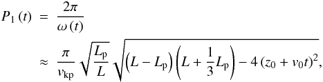 (23)which we have explicitly written in terms of the dimensional time, t, and the flow velocity, v0. By using Eq. (23) along with observational values of the period, it is possible to give an estimation of L, i.e., the total length of the flux tube, which is a parameter difficult to measure from the observations. Let us assume that we have performed an observation of a transversely oscillating and flowing thread with a good cadence and we have determined the evolution of the period with time. For convenience, we set t = 0 when the maximum of the period takes place, namely P1(0), so we can also fix z0 = 0 in Eq. (23). Then, we denote as P1(τ) the instantaneous period measured at t = τ. We use Eq. (23) and compute the ratio P1(τ)/P1(0) to find an estimation of the length of the magnetic flux tube as
 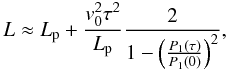 (24)where again we assumed that the flow velocity is slow. We see that the right-hand side of Eq. (24) depends on quantities that can be directly measured from the observations. As an example, let us assume the following values: P1(τ)/P1(0) = 0.9, v0 = 40 km s-1, Lp = 10 000 km, and τ = 5 min. From Eq. (24) we obtain L ≈ 1.6 × 10⁵ km. However, the accuracy of Eq. (24) is limited by the uncertainties and error bars of the observations. In particular, a very accurate determination of the ratio P1(τ)/P1(0) is needed. For instance, a 10% uncertainty of P1(τ)/P1(0) produces a 85% uncertainty of L when propagation of errors is used in Eq. (24) and the remaining parameters are kept constant. This makes a reliable application of Eq. (24) difficult in practice.
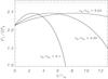 |
Fig. 4 Ratio P1/2P2 of a flowing thread with Lp/L = 0.1 and z0/L = −0.25 for v0/vAp = 0.03, 0.05, 0.1. The dotted line is the result from Eq. (25) in the case without flow and for a prominence thread located at the center of the magnetic structure. |
Another relevant parameter that can give us a seismological determination of L is the ratio P1/2P2, where P2 is the period of the first harmonic. The deviation of this ratio from unity is an indication of the longitudinal inhomogeneity length scale of the magnetic tube. Its application was used for the first time in the context of coronal loop oscillations by Andries et al. (2005a,b) and has been explored in subsequent works (see the recent review by Andries et al. 2009, and references therein). In prominence thread oscillations, Díaz et al. (2010) explored the importance of the ratio P1/2P2 to estimate Lp/L in static threads. While in coronal loops P1/2P2 < 1, Díaz et al. (2010) found that in prominence threads P1/2P2 > 1. The reason for this result is that in prominence threads mass density is arranged just in the opposite way to that in coronal loops. In loops the density is larger in the footpoints than in the apex due to gravitational stratification, while in prominence threads the density is much larger in the center of the magnetic tube because of the presence of the prominence material.
For a large density contrast between the prominence and the coronal plasmas, and assuming that the thread is located at the center of the magnetic cylinder, the relation between P1/2P2 and Lp/L obtained by Díaz et al. (2010) in their Eq. (11) is 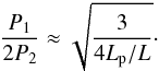 (25)Let us see how the ratio P1/2P2 is affected by the flow and so how the results of Díaz et al. (2010) are modified. However, it is difficult to obtain an analytical expression for P2 when flow is present. Instead, we compute both P1 and P2 by solving Eq. (14) with numerical methods. Figure 4 shows P1/2P2 as a function of time for Lp/L = 0.1 and z0/L = −0.25, and for different values of v0/vAp. The numerical results are compared with the analytical expression of Díaz et al. (2010). First of all, we see that the period ratio is strongly influenced by the velocity at which the prominence thread flows along the flux tube. P1/2P2 is maximal when the thread in centered within the tube (P1/2P2 ≈ 2.5 for the particular set of parameter in Fig. 4) and P1/2P2 → 1 when the thread reaches the footpoint. The analytical approximation of Díaz et al. (2010) for the static case gives a larger value of P1/2P2 in comparison to the case with flow. This means that flow reduces the period ratio. Therefore, Eqs. (24) and (25) could be used together to obtain a more accurate determination of the magnetic tube length, as the value of L inferred from Eq. (25) should be considered as a upper bound for this parameter.
4. Numerical results: time-dependent simulations
Here, we compare the analytical results of the WKB approximation with the full numerical solution of the time-dependent problem. We use the PDE2D code (Sewell 2005) for that purpose. The set-up of the numerical code is similar to that of Terradas et al. (2008). Equation (1) is integrated assuming the boundary conditions vr(± L/2,t) = 0. An initial condition for vr at t = 0 is also provided. In the code, the distances are expressed in units of L and the velocities in units of the prominence Alfvén speed, . We take L = 105 km. Assuming B = 50 G and ρp = 10-10 kg m-3 as realistic values in active region prominences, we obtain vAp ≈ 446 km s-1. The flow velocities on the plane of sky estimated by Okamoto et al. (2007) are in the interval between 15 km -1 to 46 km s-1. Hence in our simulations we consider values for the ratio v0/vAp in the range 0.03 ≲ v0/vAp ≲ 0.1. In the code, time is expressed in units of the Alfvén travel time, i.e., τAp = L/vAp ≈ 3.74 min. In addition, in all the following computations we have used ρp/ρc = 200 and ρe/ρc = 1.
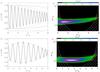 |
Fig. 5 a) vr at z = 0 (solid line in arbitrary units) as a function of time in a prominence fine structure with Lp/L = 0.1, v0/vAp = 0.05, and z0 = 0. The initial excitation is the fundamental kink mode eigenfunction for v0 = 0. The dashed line is the amplitude in the WKB approximation (Eq. (22)), while the dotted line corresponds to the fit proposed in Eq. (26) with n = 1. b) Wavelet power spectrum for the dimensionless period, P/τAp, corresponding to the signal displayed in panel a). The white dashed line is the period in the WKB approximation (Eq. (23)), whereas the horizontal dotted line is the period at t = 0. The red solid line denotes 99% of confidence level. c) Same as panel a) but for Lp/L = 0.2, v0/vAp = 0.1, and z0/L = −0.25. d) Same as panel b) but for the signal of panel c), and with the horizontal dotted line denoting the maximum of the period. |
4.1. Excitation of the fundamental mode
First, we use the eigenfunction of the fundamental kink mode as the initial condition for vr at t = 0. The eigenfunction is obtained by solving the dispersion relation of the normal mode problem and computing the spatial distribution of the corresponding perturbation (see details in Dymova & Ruderman 2005; Soler et al. 2010; Díaz et al. 2010). Hence, we make sure that, after the initial excitation, the magnetic tube mainly oscillates in its fundamental mode.
As a check of the numerical code, we consider the static case and put the thread at the center of the magnetic tube, i.e., v0 = 0 and z0 = 0. In this test simulation, we take Lp/L = 0.1. By looking at the time-dependent evolution of vr, we check that the magnetic tube oscillates as a whole. A plot of vr at z = 0 as a function of time (not displayed here for the sake of simplicity) shows that the amplitude of the oscillation is constant during the whole duration of the simulation, meaning that numerical dissipation is negligible in the simulation. Later, we perform a power spectrum of vr at z = 0 (see, e.g., Carbonell & Ballester 1991) and find a large peak centered around the fundamental normal mode frequency. The maximum of the power spectrum agrees very well with the approximate frequency of the normal mode given by Eq. (16). For the set of parameters used in this numerical test, the period in dimensional units is P ≈ 2.6 min. We have performed similar simulations but using different values of Lp/L and z0. Equivalent results to those commented before have been obtained in all cases. This indicates, on the one hand, that the normal mode interpretation is a very good representation for the time-dependent evolution of the oscillation in the static case and, on the other hand, that the numerical code works properly.
Hereafter, we incorporate the effect of the flow. First, we fix Lp/L = 0.1 and z0 = 0, and consider v0/vAp = 0.05. In this situation, the thread is initially located at the center of the magnetic tube. We make sure that the simulation stops before the threads reaches the photospheric wall. We plot in Fig. 5a the radial velocity perturbation at z = 0 as a function of time. Contrary to the static case, now the amplitude of the oscillation decreases in time as the thread moves from the center towards the end of the magnetic tube. This behavior is qualitatively described by Eq. (22) obtained in the WKB approximation (see dashed line in Fig. 5a), although Eq. (22) underestimates the actual decrease of the amplitude. Inspired by Eq. (22), we propose the following fit for the amplitude, ![\begin{eqnarray} Q_1 (z,t_1) &=& Q_0(z) \left[ \frac{\left( L - \lp \right) \left( L + \frac{1}{3} \lp \right) - 4 \left( z_0 + t_1 L \right)^2}{\left( L - \lp \right) \left( L + \frac{1}{3} \lp \right) - 4 z_0^2} \right]^{n},\label{eq:fit} \end{eqnarray}](/articles/aa/full_html/2011/07/aa16536-11/aa16536-11-eq152.png) (26)with n an empirical exponent. When Eq. (26) is applied to the results of Fig. 5a, we obtain that the exponent n = 1 provides a good fit for the amplitude (see the dotted line in Fig. 5a).
(26)with n an empirical exponent. When Eq. (26) is applied to the results of Fig. 5a, we obtain that the exponent n = 1 provides a good fit for the amplitude (see the dotted line in Fig. 5a).
On the other hand, we perform in Fig. 5b a wavelet power spectrum (Torrence & Compo 1998) of the signal displayed in Fig. 5a. We find that the period decreases in time as the thread moves towards the footpoint of the magnetic structure. The WKB approximation for the period given by Eq. (23) is in excellent agreement with the position of the maximum of the wavelet spectrum (see dashed line in Fig. 5b). As discussed in Sect. 3.2, the WKB approximation for the period is much more accurate than the WKB approximation for the amplitude. In addition, we see that the rate at which the period changes with respect to the value at t = 0 is not constant. Using Eq. (23) and considering the parameters of this particular simulation, the period of the oscillation when the thread is at z = L/4 has decreased of about 9% with the respect to its initial value at z = 0, whereas the period decreases of about 45% when the thread finally reaches the footpoint of the magnetic tube at z = L.
We repeat the simulation for Lp/L = 0.2 and a faster flow, v0/vAp = 0.1, and take z0/L = −0.25 to consider the thread initially displaced from the center of the flux tube. The radial velocity perturbation at z = 0 is plotted in Fig. 5c, and the corresponding wavelet power spectrum is shown in Fig. 5d. These results are equivalent to those of Figs. 5a, b, i.e., both the amplitude and the period of the oscillation depend on the position of the prominence thread within the flux tube, taking both of them their maximum value when the thread is centered. As before, Eq. (23) is a very good approximation to the period.
4.2. Arbitrary excitation
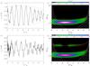 |
Fig. 6 a) Same as Fig. 5c but for a initial excitation given by Eq. (27) with ζ/L = −0.25 and σ/L = 0.2. b) Wavelet power spectrum corresponding to the signal displayed in panel a). c) Same as panel a) but for ζ/L = 0 and σ/L = 0.2. d) Same as panel b) but for the signal displayed in panel c), with the dash-dotted line denoting the period of the first harmonic. |
In the previous section, we have used an initial condition for vr that corresponds to the fundamental mode eigenfunction, so only this mode is excited. However, it is expected that the energy from an arbitrary disturbance of the flux tube is deposited in many normal modes (see a discussion on this issue in, e.g., Terradas et al. 2007). To represent an arbitrary disturbance of the flux tube, we consider a Gaussian function as the initial condition of vr at t = 0, namely ![\begin{equation} v_r (z,t=0) = \exp \left[ - \frac{\left( z - \zeta \right)^2}{\sigma^2} \right], \label{eq:excitat} \end{equation}](/articles/aa/full_html/2011/07/aa16536-11/aa16536-11-eq161.png) (27)where ζ and σ are arbitrary parameters. Whereas ζ correspond to the position of the maximum of the excitation, σ determines its width.
(27)where ζ and σ are arbitrary parameters. Whereas ζ correspond to the position of the maximum of the excitation, σ determines its width.
In the following simulations, we consider the same model parameters as in Figs. 5c, d, i.e., Lp/L = 0.2, v0/vAp = 0.1, and z0/L = −0.25, but use the initial condition given by Eq. (27). To begin with, we take σ/L = 0.2 and consider different values of ζ. First we use ζ/L = −0.25, so the excitation is mainly confined to the dense prominence region of the flux tube. The result of this simulation is displayed in Fig. 6a, which shows the evolution in time of vr at z = 0, whereas Fig. 6b shows the corresponding wavelet power spectrum. It is interesting to compare Figs. 5d and 6b to see that, in the present case, the oscillation dynamics is still governed by the fundamental normal mode. We see in Fig. 6a that there is some contribution of higher harmonics to the behavior of vr in time, although their contribution to the overall oscillation is of very minor importance. In addition, the evolution of the amplitude of vr remains qualitatively described by Eq. (26) with n = 1.
Next, we perform another simulation by taking the same parameters as before but assuming ζ/L = 0. In this case, the maximum of the initial excitation is located in the evacuated part of the magnetic tube. Again, we plot in Fig. 6c vr at z = 0 versus time, and in Fig. 6d the wavelet power spectrum. The behavior of vr in time is substantially different in the present situation compared to the case of Figs. 6a, b. First of all, we see that vr is not governed by the fundamental mode exclusively. The wavelet power spectrum indicates that the energy from the initial disturbance is mainly deposited to the fundamental mode, but also the first harmonic is excited. The dependence in time of the fundamental mode period is again well described by Eq. (23). However, the contribution of the first harmonic to the overall oscillation seems to have disappeared when the thread is located at the center of the magnetic tube. The reason for this result is that the first harmonic eigenfunction has a node at z = 0 when the thread is centered, and so the first harmonic does not contribute to the signal displayed in Fig. 6c in such a case. On the other hand, it is now difficult to determine the effect of the flow on the amplitude of the oscillation.
Finally, we have performed several simulations for different values of σ. If the maximum of the excitation is located within the dense part of the flow tube, the results are rather insensitive to σ unless values much smaller than Lp are used. In all the cases, the fundamental mode is predominantly excited. However, the results are more affected by the value of σ if the maximum of the excitation is located in the evacuated part of the tube. In such a case, the larger σ, the more energy is deposited in the fundamental mode. On the contrary, as σ gets smaller the energy of the initial excitation is more distributed among higher harmonics.
The results of this section point out that the time-dependent behavior of standing kink MHD waves of flowing prominence threads is strongly influenced by the form of the initial disturbance. If the initial disturbance mainly perturbs the dense prominence part of the flux tube, the oscillations are governed by the fundamental kink mode. In such a case, the dependence of both the period and the amplitude with the flow velocity are approximately given by Eqs. (23) and (26), respectively. On the contrary, the behavior is more complicated if the initial perturbation takes place in the evacuated part of the fine structure as other harmonics are excited in addition to the fundamental mode. The contribution of the different harmonics depends on both the position and the width of the initial excitation, while the amplitude of the oscillation does not have a simple dependence on the flow velocity.
5. Discussion and conclusions
In this paper, we have investigated standing kink MHD waves in the fine structure of solar prominences, modeled as coronal magnetic flux tubes partially filled with flowing threads of prominence material. The present study extends and complements the previous work by Terradas et al. (2008), who restricted themselves to the numerical investigation of this phenomenon and did not perform an in-depth parametric study. Here, we have combined analytical methods based on the WKB approximation with time-dependent numerical simulations to assess the precise effect of the flow on both the period and the amplitude of the fundamental kink mode.
As for the effect of the flow on the period, we can distinguish two different situations. On the one hand, we find that the flow has a small effect on the period when the thread is located near the center of the supporting magnetic flux tube. In this case, the variation of the period with respect to the static case may fall within the error bars of the observations, and so the effect may be undetectable. There our results confirm the qualitative discussion of Terradas et al. (2008) about the effect of the flow on the period. On the other hand, the variation of the period is much more important when the thread approaches the footpoint of the magnetic structure. Then, the decrease of the period can be larger than 50% with respect to the static case. The case in which the thread is near one of the footpoints of the magnetic tube was not analyzed by Terradas et al. (2008).
We have also found that the flow affects the amplitude of the fundamental mode. This result was not discussed by Terradas et al. (2008). During the motion of the prominence thread along the magnetic structure, we find that the amplitude grows as the thread gets closer to the center of the tube and decreases otherwise. This produces an apparent amplification or damping of the oscillations, respectively. Observations often indicate that thread transverse oscillations are strongly damped (see, e.g., Lin 2004, 2010; Ning et al. 2009). While several mechanisms have been proposed and investigated to explain the quick attenuation (see the recent reviews by Oliver 2009; Arregui & Ballester 2010), the process of resonant absorption seems the most likely explanation (e.g., Arregui et al. 2008; Soler et al. 2009a,b, 2010). Our present results indicate that the actual damping rate of the oscillations might be affected by the change of the amplitude due to the flow. This fact should be taken into account when the damping rate is used as a seismological tool to infer physical parameters of prominence threads, because the presence of flow may introduce some uncertainties on these estimations (see details in Arregui & Ballester 2010).
In addition, our numerical simulations have allowed us to determine how different perturbations excite the oscillations of the magnetic structure. Based on the cases studied in this paper, we have obtained that the fundamental mode is mostly excited when the perturbation initially disturbs the dense, prominence part of the tube. From the wavelet power spectrum of the radial velocity perturbation, we conclude that the contribution of higher harmonics is negligible, thus the overall oscillation is governed by the fundamental mode. On the contrary, a perturbation located at the evacuated part of the tube excites the fundamental mode and higher harmonics, producing a more complex behavior of the oscillations. In this last case, the effect of the flow on the amplitude is more complicated and no simple dependence can be extracted from the simulations.
This paper has explored the properties of MHD waves in a coronal magnetic structure with a changing configuration. Previous similar works in this line are, e.g., Terradas et al. (2008) in prominences, and Morton et al. (2010); Morton & Erdélyi (2010a,b) in coronal loops. During the revision of this paper it also came to our knowledge the recent work by Ruderman (2011). In view of the highly dynamic nature of the coronal medium in general, and the prominence plasma in particular, this kind of modeling represents a better description of the actual oscillatory phenomena in the corona and in prominences. The present investigation could be extended in the future by incorporating the effect of the density inhomogeneity in the transverse direction and so investigating the resonant damping of the kink mode.
Acknowledgments
R.S. thanks J. L. Ballester, R. Oliver, and T. Van Doorsselaere for useful comments. R.S. acknowledges support from a Marie Curie Intra-European Fellowship within the European Commission 7th Framework Program (PIEF-GA-2010-274716). R.S. also thanks support from the EU Research and Training Network “SOLAIRE” (MTRN-CT-2006-035484). RS acknowledges discussion within ISSI Team on “Solar Prominence Formation and Equilibrium: New data, new models”, and is grateful to ISSI for the financial support. M.G. acknowledges support from K.U. Leuven via GOA/2009-009. Wavelet software was provided by C. Torrence and G. Compo, and is available at http://paos.colorado.edu/research/wavelets/
References
- Ahn, K., Chae, J., Cao, W., & Goode, P. R. 2010, ApJ, 721, 74 [NASA ADS] [CrossRef] [Google Scholar]
- Andries, J., Goossens, M., Hollweg, J. V., Arregui, I., & Van Doorsselaere, T. 2005a, A&A, 430, 1109 [NASA ADS] [CrossRef] [EDP Sciences] [Google Scholar]
- Andries, J., Arregui, I., & Goossens, M. 2005b, ApJ, 624, L57 [NASA ADS] [CrossRef] [Google Scholar]
- Andries, J., Van Doorsselaere, T., Roberts, B. et al. 2009, Space Sci. Rev., 149, 3 [NASA ADS] [CrossRef] [Google Scholar]
- Antolin, P., & Verwichte, E. 2011, ApJ, in press [arXiv:1105.2175] [Google Scholar]
- Arregui, I., & Ballester, J. L. 2010, Space Sci. Rev., in press, DOI:10.1007/s11214-010-9648-9 [Google Scholar]
- Arregui, I., Terradas, J., Oliver, R., & Ballester, J. L. 2008, ApJ, 682, L141 [NASA ADS] [CrossRef] [Google Scholar]
- Ballester, J. L. 2006, Phil. Trans. R. Soc. A, 364, 405 [NASA ADS] [CrossRef] [Google Scholar]
- Bender, C. M., & Orszag, S. A. 1978, Advanced Mathematical Methods for Scientists and Engineers (New York: McGraw-Hill) [Google Scholar]
- Berger, T. E., Shine, R. A., Slater, G. L., et al. 2008, ApJ, 676, L89 [Google Scholar]
- Cao, W., Ning, Z., Goode, P. R., Yurchyshyn, V., & Haisheng, J. 2010, ApJ, 719, L95 [NASA ADS] [CrossRef] [Google Scholar]
- Carbonell, M., & Ballester, J. L. 1991, A&A, 249, 295 [NASA ADS] [Google Scholar]
- Chae, J. 2010, ApJ, 714, 618 [NASA ADS] [CrossRef] [Google Scholar]
- Chae, J., Ahn, K., Lim, E.-K., Choe, G. S., & Sakurai, T. 2008, ApJ, 689, L73 [NASA ADS] [CrossRef] [Google Scholar]
- De Pontieu, B., & McIntosh, S. W. 2010, ApJ, 722, 1013 [NASA ADS] [CrossRef] [Google Scholar]
- Díaz, A. J., Oliver R., Erdélyi, R., & Ballester, J. L. 2001, A&A, 379, 1083 [NASA ADS] [CrossRef] [EDP Sciences] [Google Scholar]
- Díaz, A. J., Oliver R., & Ballester, J. L. 2002, ApJ, 580, 550 [NASA ADS] [CrossRef] [Google Scholar]
- Díaz, A. J., Oliver R., & Ballester, J. L. 2010, ApJ, 725, 1742 [NASA ADS] [CrossRef] [Google Scholar]
- Dymova, M. V., & Ruderman, M. S. 2005, Sol. Phys., 229, 79 [NASA ADS] [CrossRef] [Google Scholar]
- Edwin, P. M., & Roberts, B. 1983, Sol. Phys., 88, 179 [NASA ADS] [CrossRef] [Google Scholar]
- Erdélyi, R., & Fedun, V. 2007, Science, 318, 1572 [NASA ADS] [CrossRef] [PubMed] [Google Scholar]
- Goedbloed, H., & Poedts, S. 2004, Principles of magnetohydrodynamics (Cambridge University Press) [Google Scholar]
- Goossens, M., Terradas, J., Andries, J., Arregui, I., & Ballester, J. L. 2009, A&A, 503, 213 [NASA ADS] [CrossRef] [EDP Sciences] [Google Scholar]
- Jess, D. B., Mathioudakis, M., Erdélyi, R., et al. 2009, Science, 323, 1582 [NASA ADS] [CrossRef] [PubMed] [Google Scholar]
- Joarder, P. S., & Roberts, B. 1992, A&A, 261, 625 [NASA ADS] [Google Scholar]
- Joarder, P. S., Nakariakov, V. M., & Roberts, B. 1997, Sol. Phys., 173, 81 [NASA ADS] [CrossRef] [Google Scholar]
- Kucera, T. A., Tovar, M., & De Pontieu, B. 2003, Sol. Phys., 212, 81 [NASA ADS] [CrossRef] [Google Scholar]
- Lin, Y. 2004, PhD Thesis, University of Oslo, Norway [Google Scholar]
- Lin, Y. 2010, Space Sci. Rev., in press, DOI:10.1007/s11214-010-9672-9 [Google Scholar]
- Lin, Y., Engvold, O., & Wiik, J. E. 2003, Sol. Phys., 216, 109 [NASA ADS] [CrossRef] [Google Scholar]
- Lin, Y., Martin, S. F., & Engvold, O. 2008, in Subsurface and Atmospheric Influences on Solar Activity, ed. R. Howe, R. W. Komm, K. S. Balasubramaniam, & G. J. D. Petrie (San Francisco: ASP), ASP Conf. Ser. 383, 235 [Google Scholar]
- Lin, Y., Soler, R., Engvold, O., et al. 2009, ApJ, 704, 870 [NASA ADS] [CrossRef] [Google Scholar]
- Morton, R. J., & Erdélyi, R. 2010a, ApJ, 707, 750 [Google Scholar]
- Morton, R. J., & Erdélyi, R. 2010b, A&A, 519, A43 [NASA ADS] [CrossRef] [EDP Sciences] [Google Scholar]
- Morton, R. J., Hood, A. W., & Erdélyi, R. 2010, A&A, 512, A23 [NASA ADS] [CrossRef] [EDP Sciences] [Google Scholar]
- Nakariakov, V. M., & Roberts, B. 1995, Sol. Phys., 159, 213 [NASA ADS] [CrossRef] [Google Scholar]
- Ning, Z., Cao, W., Okamoto, T. J., Ichimoto, K., & Qu, Z. Q. 2009, A&A, 499, 595 [NASA ADS] [CrossRef] [EDP Sciences] [Google Scholar]
- Ofman, L., & Wang, T. J. 2008, A&A, 482, L9 [NASA ADS] [CrossRef] [EDP Sciences] [Google Scholar]
- Okamoto T. J., Tsuneta, S., Berger, T. E., et al. 2007, Science, 318, 1557 [Google Scholar]
- Oliver, R. 2009, Space Sci. Rev., 149, 175 [NASA ADS] [CrossRef] [Google Scholar]
- Oliver, R., Ballester, J. L., Hood, A. W., & Priest, E. R. 1993, ApJ, 409, 809 [NASA ADS] [CrossRef] [Google Scholar]
- Ruderman, M. S. 2011, Sol. Phys., in press, DOI:10.1007/s11207-011-9772-z [Google Scholar]
- Schmieder, B., Chandra, R., Berlicki, A., & Mein, P. 2010, A&A, 514, A68 [NASA ADS] [CrossRef] [EDP Sciences] [Google Scholar]
- Sewell, G. 2005, The Numerical Solution of Ordinary and Partial Differential Equations (Hoboken: Wiley & Sons) [Google Scholar]
- Soler, R., Oliver, R., Ballester, J. L., & Goossens, M. 2009a, ApJ, 695, L166 [NASA ADS] [CrossRef] [Google Scholar]
- Soler, R., Oliver, R., & Ballester, J. L. 2009b, ApJ, 707, 662 [NASA ADS] [CrossRef] [Google Scholar]
- Soler, R., Arregui, I., Oliver, R., & Ballester, J. L. 2010, ApJ, 722, 1778 [NASA ADS] [CrossRef] [Google Scholar]
- Terradas, J., Andries, J., & Goossens, M. 2007, A&A, 469, 1135 [NASA ADS] [CrossRef] [EDP Sciences] [Google Scholar]
- Terradas, J., Arregui, I., Oliver, R., & Ballester, J. L. 2008, ApJ, 678, L153 [NASA ADS] [CrossRef] [Google Scholar]
- Terradas, J., Goossens, M., & Verth, G. 2010, A&A, 524, A23 [NASA ADS] [CrossRef] [EDP Sciences] [Google Scholar]
- Terradas, J., Arregui, I., Verth, G., & Goossens, M. 2011, ApJ, 729, L22 [NASA ADS] [CrossRef] [Google Scholar]
- Terra-Homem, M., Erdélyi, R., & Ballai, I. 2003, Sol. Phys., 217, 199 [NASA ADS] [CrossRef] [Google Scholar]
- Tomczyk, S., & McIntosh, S. W. 2010, ApJ, 697, 1384 [Google Scholar]
- Tomczyk, S., McIntosh, S. W., Keil, S. L., et al. 2007, Science, 317, 1192 [NASA ADS] [CrossRef] [PubMed] [Google Scholar]
- Torrence, C., & Compo, G. P. 1998, Bull. Amer. Meteor. Soc., 79, 61 [CrossRef] [Google Scholar]
- Van Doorsselaere, T., Nakariakov, V. M., & Verwichte, E. 2008, ApJ, 676, L73 [NASA ADS] [CrossRef] [Google Scholar]
- Verth, G., Terradas, J., & Goossens, M. 2010, ApJ, 718, L102 [NASA ADS] [CrossRef] [Google Scholar]
- Wang, Y.-M. 1999, ApJ, 520, L71 [NASA ADS] [CrossRef] [Google Scholar]
- Wang, T. J., Ofman, L., Davila, J. M., & Mariska, J. T. 2009, A&A, 503, L25 [NASA ADS] [CrossRef] [EDP Sciences] [Google Scholar]
- Zirker, J. B., Engvold, O., & Martin, S. F. 1998, Nature, 396, 440 [NASA ADS] [CrossRef] [Google Scholar]
All Figures
|
Fig. 1 Sketch of the prominence fine structure model adopted in this work. |
| In the text | |
|
Fig. 2 Dimensionless frequency, ωτAp, versus time in units of the internal Alfvén travel time, τAp = L/vAp. Results corresponding to the fundamental mode and the lowest seven harmonics obtained by numerically solving Eq. (14) for a flowing thread with Lp/L = 0.1, v0/vAp = 0.05, and z0/L = −0.25. The vertical dotted line denotes the time when the prominence thread is centered within the flux tube. |
| In the text | |
|
Fig. 3 Dimensionless frequency, ωτAp, versus time in units of the internal Alfvén travel time, τAp = L/vAp, for a) Lp/L = 0.05, 0.1, 0.2 with v0/vAp = 0.05, and b) v0/vAp = 0.03, 0.05, 0.1 with Lp/L = 0.1. In all cases, z0/L = −0.25. The solid lines are the results obtained by numerically solving Eq. (14), whereas the symbols correspond to the analytical approximation given by Eq. (16). The vertical dotted line in panel a) denotes the minimum of the curves, i.e., the time when the prominence thread is centered within the flux tube. |
| In the text | |
|
Fig. 4 Ratio P1/2P2 of a flowing thread with Lp/L = 0.1 and z0/L = −0.25 for v0/vAp = 0.03, 0.05, 0.1. The dotted line is the result from Eq. (25) in the case without flow and for a prominence thread located at the center of the magnetic structure. |
| In the text | |
|
Fig. 5 a) vr at z = 0 (solid line in arbitrary units) as a function of time in a prominence fine structure with Lp/L = 0.1, v0/vAp = 0.05, and z0 = 0. The initial excitation is the fundamental kink mode eigenfunction for v0 = 0. The dashed line is the amplitude in the WKB approximation (Eq. (22)), while the dotted line corresponds to the fit proposed in Eq. (26) with n = 1. b) Wavelet power spectrum for the dimensionless period, P/τAp, corresponding to the signal displayed in panel a). The white dashed line is the period in the WKB approximation (Eq. (23)), whereas the horizontal dotted line is the period at t = 0. The red solid line denotes 99% of confidence level. c) Same as panel a) but for Lp/L = 0.2, v0/vAp = 0.1, and z0/L = −0.25. d) Same as panel b) but for the signal of panel c), and with the horizontal dotted line denoting the maximum of the period. |
| In the text | |
|
Fig. 6 a) Same as Fig. 5c but for a initial excitation given by Eq. (27) with ζ/L = −0.25 and σ/L = 0.2. b) Wavelet power spectrum corresponding to the signal displayed in panel a). c) Same as panel a) but for ζ/L = 0 and σ/L = 0.2. d) Same as panel b) but for the signal displayed in panel c), with the dash-dotted line denoting the period of the first harmonic. |
| In the text | |
Current usage metrics show cumulative count of Article Views (full-text article views including HTML views, PDF and ePub downloads, according to the available data) and Abstracts Views on Vision4Press platform.
Data correspond to usage on the plateform after 2015. The current usage metrics is available 48-96 hours after online publication and is updated daily on week days.
Initial download of the metrics may take a while.