| Issue |
A&A
Volume 530, June 2011
|
|
|---|---|---|
| Article Number | A46 | |
| Number of page(s) | 11 | |
| Section | Planets and planetary systems | |
| DOI | https://doi.org/10.1051/0004-6361/201016282 | |
| Published online | 05 May 2011 | |
Last giant impact on the Neptunian system
Constraints on oligarchic masses in the trans-Saturnian region
1
Instituto Argentino de Radioastronomía (IAR-CONICET),
C.C. No 5,
1894
Villa Elisa,
Argentina
e-mail: This email address is being protected from spambots. You need JavaScript enabled to view it.
2 Facultad de Ciencias Astronómicas y Geofísicas, Universidad
Nacional de La Plata, Argentina
3
Departamento de Astronomía, Universidad de Chile,
Casilla 36-D, Santiago, Chile
e-mail: This email address is being protected from spambots. You need JavaScript enabled to view it.
Received: 7 December 2010
Accepted: 4 February 2011
Abstract
Context. Current models of the formation of ice giants attempt to account for the formation of Uranus and Neptune within the protoplanetary disk lifetime. Many of these models calculate the formation of Uranus and Neptune in a disk that may be several times the minimum mass solar nebula model (MMSN). Modern core accretion theories assume the formation of the ice giants either in situ, or between ~10–20 AU in the framework of the Nice model. However, at present, none of these models account for the spin properties of the ice giants.
Aims. Stochastic impacts by large bodies are, at present, the usually accepted mechanisms able to account for the obliquity of the ice giants. We attempt to set constraints on giant impacts as the cause of Neptune’s current obliquity in the framework of modern theories. We also use the present orbital properties of the Neptunian irregular satellites (with the exception of Triton) to set constraints on the scenario of giant impacts at the end of Neptune formation.
Methods. Since stochastic collisions among embryos are assumed to occur beyond oligarchy, we model the angular momentum transfer to proto-Neptune and the impulse transfer to its irregular satellites by the last stochastic collision (GC) between the protoplanet and an oligarchic mass at the end of Neptune’s formation. We assume a minimum oligarchic mass mi of 1 m⊕.
Results. From angular momentum considerations, we obtain that an oligarchic mass mi ~ 1 m⊕ ≤ mi ≤ 4 m⊕ would be required at the GC to reproduce the present rotational properties of Neptune. An impact with mi > 4 m⊕ is not possible, unless the impact parameter of the collision were very small. This result is invariant either Neptune had formed in situ or between 10–20 AU and does not depend on the occurrence of the GC after or during the possible migration of the planet. From impulse considerations, we find that an oligarchic mass mi ~ 1 m⊕ ≤ mi ≤ 1.4 m⊕ at the GC is required to keep or capture the present population of irregular satellites. If mi had been higher, the present Neptunian irregular satellites had to be formed or captured after the end of stochastic impacts.
Conclusions. The upper bounds on the oligarchic masses (4 m⊕ from the obliquity of Neptune and 1.4 m⊕ from the Neptunian irregular satellites) are independent of unknown parameters, such as the mass and distribution of the planetesimals, the location at which Uranus and Neptune were formed, the Solar Nebula initial surface mass density, and the growth regime. If stochastic impacts had occurred, these results should be understood as upper constraints on the oligarchic masses in the trans-Saturnian region at the end of ice planet formation and may be used to set constraints on planetary formation scenarios.
Key words: planets and satellites: general / planets and satellites: formation
Member of the Carrera del Investigador Científico, Consejo Nacional de Investigaciones Científicas y Técnicas (CONICET), Argentina.
Fellow of the Comisión Nacional de Investigación Científica y Tecnológica (CONICYT), Chile.
© ESO, 2011
1. Introduction
The origin of the rotational properties of the planets in the Solar System is one of the fundamental questions in cosmogony. When planetesimals are accreted, they deliver rotational angular momentum caused by their relative motion with respect to the protoplanet. The angular momentum, L, acquired in an individual collision can be in any direction. However, because of the symmetry of the system about the plane of the planet’s orbit, (z,ż) → (−z, −ż), there is no systematic preference of positive or negative Lx or Ly. An ordered component to Lz is possible, thereby producing a net planetary spin angular momentum either in the same direction as the orbital angular momentum (prograde rotation) or in the opposite direction (retrograde rotation). The angular momentum accreted from an uniform and dynamically cold disk of small planetesimals results in a slow systematic (ordered) component of planetary rotation in the retrograde direction (Lissauer & Kary 1991). Lissauer et al. (1997) have shown that systematic prograde rotation can be achieved if the disk density profiles are imposed such that the surface mass density near the outer edges of a protoplanet’s feeding zone is significantly greater than that in the rest of the accretion zone. Schlichting & Sari (2007) obtained that planetesimals close to a meter in size, are likely to collide within the protoplanet’s sphere of influence, thereby creating a prograde accretion disk around the protoplanet. The accretion of such a disk results in the formation of protoplanets spinning in the prograde sense. However, these models account for a net Lz component of the planetary spin, and the problem of the obliquity (the angle between the rotational axis of a planet and the perpendicular to its orbital plane) of the ice planets remains open.
Several theories have been proposed to account for the obliquity of giant planets. A random component of planetary rotation may be due to stochastic impacts with large bodies and may be in any direction (Lissauer & Safronov 1991; Chambers 2001). Greenberg (1974) and Kubo-Oka & Nakazawa (1995) investigated the tidal evolution of satellite orbits and examined the possibility that the orbital decay of a retrograde satellite leads to the high obliquity of Uranus, but the high mass required for the hypothetical satellite makes this very implausible. An asymmetric infall or torques from nearby mass concentrations during the collapse of the molecular cloud core leading to the formation of the Solar System could twist the total angular momentum vector of the planetary system. This twist could generate the obliquities of the outer planets (Tremaine 1991). This model has the disadvantages that the outer planets must form before the infall is complete and that the conditions for the event that would produce the twist are rather strict. The model itself is difficult to be quantitatively tested. In the Nice model of Tsiganis et al. (2005), close encounters among the giant planets produce large orbital eccentricities and inclinations that were subsequently damped to the current value by gravitational interactions with planetesimals. The obliquity changes because of the change in the orbital inclinations. Since the inclinations are damped by planetesimals interactions on timescales that are much shorter than the timescales for precession due to the torques from the Sun, especially for Uranus and Neptune, the obliquity returns to low values, if it is low before the encounters (Lee et al. 2007). Boué & Laskar (2010) reported numerical simulations showing that Uranus’s axis might be tilted during the giant planet instability phase described in the Nice model, provided that the planet has an additional satellite and a temporary large inclination being the satellite ejected after the tilt. However, the required satellite is too massive. For Saturn, a good case can be made for spin-orbit resonances (Hamilton & Ward 2004), but giant impacts in the late stages of the formation of Uranus and Neptune remain the plausible explanation for the obliquities of the ice giants (Lee et al. 2007).
If giant impacts are responsible for the obliquities of the ice planets, such impacts will strongly affect the orbits of hypothetical preexisting satellites. The impulse imparted at any collision would have produced a shift in their orbital velocity. Satellites on orbits with too large a semimajor axis escape from the system (Parisi & Brunini 1997), while satellites with a smaller semimajor axis may be pushed to outer or inner orbits acquiring greater or lower eccentricities depending on the impactor mass and velocity, the initial orbital elements, the geometry of the impact and the satellite position at the moment of impact. The present physical and dynamical properties of irregular satellites may be used to set constraints on the scenario of giant impacts at the end of the formation of ice giants (Brunini et al. 2002; Maris et al. 2007; Parisi et al. 2008).
We investigate whether our results obtained for Uranus (Parisi & Brunini 1997; Brunini et al. 2002; Parisi et al. 2008) are similar when an improved method is applied to Neptune. Since stochastic collisions among embryos are assumed to occur beyond oligarchy, we model the last stochastic collision (hereafter, GC) between the protoplanet and an oligarchic mass computing the angular momentum transfer to proto-Neptune in Sect. 2 and the impulse transfer to its irregular satellites (with the exception of Triton) in Sect. 3. In Sect. 4, we describe and discuss modern scenarios of planetary formation in the outer Solar System. The conclusions of the results are presented in Sect. 5.
2. The spin of Neptune: Angular momentum transfer to Neptune by the last giant collision (GC)
Beyond oligarchy, the final stage of planet formation consist of close encounters, collisions, and accretion events among oligarchs. Strong impacts deliver spin angular momentum to the final planet in a random-walk fashion (Lissauer & Safronov 1991). The planetary spin accumulated by successive collisions with a distribution of small or/and large planetesimals requires ad-hoc assumptions about unknown properties of the planetesimal disk, such as the mass distribution of the bodies, the velocities distribution, and the regime of growth. We avoid the necessity of quantifying these unknown parameters modeling what happened to the planet just before it acquires its present rotational status, which is our available data.
The last off-centre giant collision (GC) between proto-Neptune and the last colliding oligarch is computed assuming that the present spin properties of Neptune are acquired by the GC. The rotational parameters of the proto-Neptune prior to the GC are random; i.e., the rotational period and the spin obliquity of Neptune before the GC are unknown and taken as initial free parameters. The procedure by Parisi et al. (2008) is improved here, since no hypothesis is applied to the spin of Neptune prior to the GC. We also take the velocity of the impactor as a free parameter that is constrained from simple dynamical bounds.
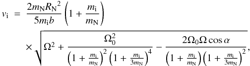
From angular momentum conservation, we get the following relation between the impactor mass mi and its incident speed vi (Parisi & Brunini 1997), assuming that the impact is inelastic (Korycansky et al. 1990):
 (1)
(1)
where b is the impact parameter of the collision, Ω the present spin angular velocity of Neptune, Ω0 the spin angular velocity that Neptune would have today if the GC had not occurred, and α is the angle between Ω and Ω0. We take a minimum value of 1 m⊕ for the oligarchic mass to impact proto-Neptune and assume a maximum oligarchic mass of 4 m⊕ for comparison.
 |
Fig. 1 Impactor incident speed vi as a function of the initial period T0 for mi = 1 m⊕, obtained through angular momentum transfer for the most probable impact parameter b = 2/3 Rc. a) α = 0°, b) α = 29.58°, c) α = 60°, d α = 90°, e) α = 130°, and f) α = 170°. The upper constraint on vi (viM) is depicted by dotted lines while the lower constraint on vi (vim) is shown by dashed lines. viM and vim are obtained from simple dynamical constraints. |
Break-up period of proto-Neptune before the GC for different impactor masses.
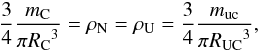
We get Neptune data from the JPL homepage. The current radius of Neptune RN is taken as 24 764 km and the mass of Neptune after the GC, (mi + mN), is taken as its current mass of 102.44 × 1024 kg. The spin period of Neptune is T = 16.11 h, thus Ω = 1.08338 × 10⁻⁴ s-1 (Ω = 2π/T). Neptune’s current obliquity is 29.58°. In the single stochastic impact approach α = 29.58°. The ice to rock ratio of Neptune is 85%. Assuming that all the ice and rock are contained at the core of the planet at the time of the GC, the core mass of Neptune is ~87.074 × 1024 kg. We then compute the core radius of Neptune assuming that its core density ρN and that of Uranus ρU are the same at the end of their formation:
 (2)
(2)
where muc = 74.737 × 1024 kg is the core mass of Uranus (Parisi & Brunini 1997) and RUC = 1.8 × 10⁴ km its core radius (Bodeheimer & Pollak 1986). From Eq. (2), we get the core radius of Neptune, RC = 1.9 × 10⁴ km. At the end of the formation of Uranus and Neptune, their gas envelopes extend until the accretion radius (e.g. Bodenheimer & Pollack 1986). Then, the radius of Neptune is ~2.724 × 10⁷ km (1100 RN), whereas its core containing most of the mass has a radius of only 1.9 × 10⁴ km. In this situation, a collision onto the core is necessary for an inelastic collision to occur and to impart the required angular momentum (Korycansky et al. 1990). Since b is an unknown quantity, we take its most probable value: b = (2/3)RC (Parisi et al. 2008).
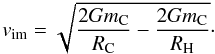
To set constraints on the impactor speed vi, we calculated the lower bound of vi (vim) corresponding to a body within the Hill radius RH of Neptune and undergoing a free fall towards Neptune’s core:
 (3)
(3)
The second term of Eq. (3) is negligible, and then, vim ~ 24.758 km s-1.
The upper bound of vi (viM) for a body bound to the Solar System corresponds to a parabolic orbit with the impactor lying on the same orbital plane as proto-Neptune and moving in a direction opposite to Neptune’s motion, including the acceleration caused by the planet (Parisi & Brunini 1997):
![Mathematical equation: \begin{equation} v_{\rm iM}=\sqrt{\left[\sqrt{\frac{2GM_{\odot}}{a_{\rm N}}}+ \sqrt{\frac{GM_{\odot}}{a_{\rm N}}} \right]^{2}+ \frac{2GM_{\rm N}}{R_{\rm C}}}, \label{vp} \end{equation}](/articles/aa/full_html/2011/06/aa16282-10/aa16282-10-eq55.png) (4)
(4)
where M⊙ is the mass of the Sun and aN the Neptunian orbital semiaxis at the time of the GC. Assuming that the GC with Neptune occurred at 30 AU, viM is ~30 km s-1. If Neptune had been formed between 12 and 30 AU (Dodson-Robinson & Bodenheimer 2010; Benvenuto et al. 2009) and the GC had occurred before or during outward migration (Tsiganis et al. 2005), viM would had been between 35 and 30 km s-1. It should be noted that our estimate of viM in Eq. (4) must be taken with care since big bodies velocity dispersion may increase so much that some fraction of them in the outer Solar System are ejected. Then, we take a maximum possible value for viM of ~40 km s-1.
We computed vi as a function of T0 (T0 = 2π/Ω0) through Eq. (1) for mi 1, 2.7, and 4 m⊕. Since α is a free parameter, we took six values of α: 0°, 29.58°, 60°, 90°, 130°, and 170°. For α between 180° and 360°, the results would be the same as for the interval [0°, 180°] since Eq. (1) is an even function of α. The cases with α ≥ 60° are less probable since it requires a very high initial obliquity before the GC. For each α, vi(T0) must fall between the bounds given by vim and viM. In Fig. 1, we show the results for mi = 1 m⊕. The permitted values of T0 for α = 0° (Fig. 1a) are between 6.95 h and 8.80 h and T0 > 43.70 h. If the present obliquity of Neptune was caused by a single stochastic impact (Fig. 1b), the permitted values of T0 are between 7.87 h and 11.14 h, and T0 > 34.52 h. In Fig. 1c, T0 must be greater than 12.29 h. If α ≥ 90°, T0 must be greater than 30 h. The curves shift up and right as α increases. In Fig. 2, we display the same as in Fig. 1 for mi = 2.7 m⊕. The intervals of permitted T0 are [3.15, 4.49] h for α = 0° (Fig. 2a) and [6.28, 15.66] h for α = 170° (Fig. 2f). For intermediate α, the range of permitted T0 falls between both cases. In Fig. 3, we show the results for mi = 4 m⊕, where we can see that the permitted T0 are very low1. Then, we calculate the break-up speed Ω0b given by
 (5)
(5)
where RN0 = RN/(1 + mi/3mN) (Parisi & Brunini 1997).
From Eq. (5), we get the period Tob (2π/Ω0b) tabulated in Table 1. If T0 < Tob, the planet breaks up since centrifugal forces exceed gravitational forces. We then discard the cases shown in Fig. 3a–c since the permitted T0 are very close to Tob = 3.43 h. It should be noted that the curves of vi in Figs. 1–3 shift to the left side as mi increases. Also, the cases for α ≥ 60° are unlikely, since a very high initial obliquity would be required. Then, for an impactor mass mi > 4 m⊕ the permitted T0 diminishes, while Tob increases (see Table 1). This implies that an impactor mass mi > 4 m⊕ would refute the GC hypothesis since T0 is less than Tob unless α is very large or b ≪ 2/3 RC. However, the probability that b < RC/3 is 0.1 and may be discarded. For b between RC/3 and 2/3RC, the probability is 0.33, and it cannot be discarded. However, for these values of b, the curves of Fig. 3 shift upwards by a factor between 1 and 2, and the permitted T0 remain lower than five hours for Figs. 3a, b. Thus, even for b between RC/3 and 2/3RC, the permitted T0 are close to Tob unless α is large. Moreover, if the impactor is large, the most probable impact parameter is b = 2/3(Rc + R) (R is the impactor radius). Then, the probability that b were less than 2/3 Rc would be even lower.
We may then conclude that an impact with a mass higher than 4 m⊕ probably could not have occurred since it would be improbable that it could reproduce the present rotational properties of Neptune. It might be understood as an upper bound for the oligarchic masses in the trans-Saturnian region at the end of Neptune formation.
3. Irregular satellites: may they set constraints on giant impacts?
3.1. Their origin: how and when irregular satellites of giant planets were captured remains open
Rich systems of irregular satellites of the giant planets have been discovered very recently. The study of their origin is very important because it can provide constraints on the formation process of giant planets and may probe the properties of the primordial planetesimal disk (Parisi et al. 2008; Vokrouhlicky et al. 2008). Neptune has at present seven irregular satellites: I Triton, II Nereid, IX Halimede, XI Sao, XII Laomedeia, XIII Neso, and X Psamathe (Holman et al. 2004; Sheppard et al. 2006b). Some of their physical and orbital parameters are shown in Table 2.
Irregular satellites of giant planets are characterized by eccentric (highly tilted with respect to the parent planet equatorial plane) and in some case retrograde, orbits. These objects cannot have formed by circumplanetary accretion as the regular satellites but they are likely products of an early capture of primordial objects from heliocentric orbits, probably in association with planet formation itself (Jewitt & Sheppard 2005). It is possible for an object circling the sun to be temporarily trapped by a planet. In terms of the classical three-body problem, this type of capture can occur when the object passes through the interior Lagrangian point, L2, with a very low relative velocity. But, without any other mechanism, such a capture is not permanent and the objects will eventually return to a solar orbit after several or several hundred orbital periods. To turn a temporary capture into a permanent one requires a source of orbital energy dissipation and needs for particles to remain inside the Hill sphere long enough for the capture to be effective. Although giant planets currently have no efficient mechanism of energy dissipation for permanent capture, several mechanisms may have operated at their formation epoch: 1) gas drag in the solar nebula or in an extended, primordial planetary atmosphere or in a circumplanetary disk (Pollack et al.1979; Cuk & Burns 2003); 2) pull-down capture caused by the mass growth and/or orbital expansion of the planet, which expands its Hill sphere (Brunini 1995; Heppenheimer & Porco 1977); 3) collisional interaction between two planetesimals passing near the planet or between a planetesimal and a regular satellite. This mechanism, the so-called break-up process, leads to the formation of dynamical groupings (e.g. Colombo & Franklin 1971; Nesvorny et al. 2004). After a break-up the resulting fragments of each progenitor form a population of irregular satellites with similar surface composition, i.e. similar colors and irregular shapes, i.e. light curves of wide amplitude (Maris et al. 2001, 2007); 4) collisionless interactions between a massive planetary satellite and guest bodies (Tsui 1999) or between the planet and a binary object (Agnor & Hamilton 2006; Vokrouhlicky et al. 2008); 5) scattering by an eccentric Triton applicable to the Neptunian system (Goldreich et al. 1989; Cuk & Gladman 2005); and 6) collisionless interactions within the framework of the Nice model, where capture occurs during migration through three-body interactions during close encounters between the giant planets (Nesvorny et al. 2007; Bottke et al. 2010). There might have been several encounters and stochastic collisions among protoplanets during migration, all of which could have both removed and captured irregular satellites. It was shown that the last captured population of irregular satellites by three-body encounters in the framework of the Nice model were very likely significantly larger than what we observe today. These populations had then experienced rapid collisional evolution and almost self destructed, evolving into quasi-steady state size frequency distributions with extremely shallow power-law slopes for D > 10 km (Bottke et al. 2010).
Orbital and physical parameters of the Neptunian irregulars taken from JPL (http://ssd.jpl.nasa.gov).
The knowledge of colors and of the size and shape distribution of irregular satellites is important for knowing their relation to the precursor population. It brings valuable clues to investigate if they are collisional fragments from break-up processes occurring at the planetesimal disk and thus has nothing to do with how they were individually captured later by the planet, or if they are collisional fragments produced during or after the capture event (Nesvorny et al. 2003, 2007; Bottke et al. 2010). Despite many studies in past years, inconsistencies are present between colors derived by different authors for the irregular satellites of Uranus and Neptune (Maris et al. 2001, 2007; Grav et al. 2004). Moreover, if the precursors of the Uranian and Neptunian irregular satellites are objects of the Kuiper Belt or C-, P-, and D-type asteroids is still a matter of debate (Bottke et al. 2010; Levison et al. 2009). Even the recent proposed capture models run into trouble using the size frequency distribution of irregular satellites as constraints (Nesvorny et al. 2007; Bottke et al. 2010). An intensive search for fainter irregular satellites and a long term program of observations to recover light curves, colors, and phase-effect information in a self-consistent manner is needed. Constraints on the different dissipative mechanisms for the permanent capture of irregular satellites should be investigated in the framework of the different models proposed for the formation of the ice giants.
Although, recent models study the capture of irregular satellites by close encounters between giant planets in the framework of the Nice model, there is very little work on the capture and loss of irregular satellites by stochastic collisions (Parisi et al. 2008). Here, we investigate whether the present population of Neptunian irregular satellites could have been captured by stochastic impacts and/or if they could have survived to stochastic impacts. We attempt to set constraints on the occurrence of giant impacts at the end of the formation of the ice giants, on the impactor masses, and on the epoch of the capture/origin of the Neptunian irregular satellites.
3.2. The Neptunian irregular satellites were captured before, after, or during stochastic impacts?
All stochastic impacts add angular momentum to the random component of planetary spin and transfer impulse to the planet and its satellite system. Although the transfer of impulse at any collision onto the planet affects the whole system, the transfer of angular momentum affects only the rotational properties of the planet but not the orbital or rotational properties of its satellites.
The impulse accumulated by successive collisions with a distribution of small or/and large planetesimals requires ad-hoc assumptions about the unknown planetesimal mass distribution, the unknown initial surface mass density, and the unknown regime of growth. In the GC scenario, we avoid the necessity of quantifying these parameters, since we assume that the orbital properties of the irregular satellites of Neptune before the GC are unknown as are the physical and dynamical properties of oligarchs. These initial free parameters are constraint by the model from the current orbital properties of the irregular satellites and using simple general dynamical bounds.
The transfers of six of the seven irregular satellites of Neptune to their current orbits by the GC are computed following a somewhat more improved procedure than in Parisi et al. (2008). Irregular satellites may be pushed to outer or inner orbits. Moreover, they may be captured or unbound by the GC. We attempt to set constraints on their initial orbital properties, the impactor mass, and the epoch of their origin. We do not include Triton in our treatment, since this satellite is assumed to have a different origin than the other irregular satellites of Neptune owing to its high mass, small orbital semiaxis and zero orbital eccentricity (see Table 2).
Just before the GC, the square of the orbital velocity ν1 of a preexisting satellite of negligible mass is given by  (6)
(6)
where r is the position of the satellite on its orbit at the moment of the GC and a1 its orbital semiaxis.
After the GC, the satellite is transferred to another orbit with semiaxis a2 acquiring the following square of the velocity:  (7)
(7)
We set  and
and  , where A and B are arbitrary coefficients (0 < A ≤ 1, B > 0), νe being the escape velocity at r before the GC.
The semiaxis of the satellite orbit before (a1) and after (a2) the GC verify the following simple relations:
Variation in the orbital eccentricity and semiaxis (in units of RN = 24 764 km) of the Neptunian irregulars due to Solar and giant planet perturbations over a period of 105 yrs. Δamin = amean − amin and Δamax = amax − amean.
 (8)
(8)
If A < B then a1 < a2. In the special case of B = 1, the orbits are unbound from the system. If A > B then a1 > a2, the initial orbit is transferred to an inner orbit, providing a mechanism for the permanent capture of the irregular satellite even from an unbound orbit (A ≥ 1). When A = B, the orbital semiaxis remains unchanged (a1 = a2).
The position r of the satellite on its orbit at the epoch of the impact may be expressed in the following form (Bunini et al. 2002; Parisi et al. 2008): ![Mathematical equation: \begin{equation} r=\frac{2\; G\; m_{\rm N}}{(\Delta V)^2} \ \Bigg[ \frac{B'-A} { \sqrt{A} \cos{\Psi} \pm \sqrt{ (B'-A) + A \cos^2{\Psi} } } \Bigg]^2, \label{r} \end{equation}](/articles/aa/full_html/2011/06/aa16282-10/aa16282-10-eq134.png) (9)
(9)
with B′ = B(1 + mi/mN), and Ψ is the angle between ν1 and the orbital velocity change ΔV imparted to Neptune by the GC. The value of ΔV is obtained through impulse conservation considerations at collision (Parisi & Brunini 1997):
 (10)Upper bounds on a1 (a1M) and a2 (a2M) are obtained from Eqs. (8) and (9) with Ψ = 180°, i.e., assuming the impact in the direction opposite to the orbital motion of the satellites and taking the positive sign of the square root:
  (11)
(11)
The minimum eccentricity of the orbits before the collision is given by  (12)
(12)
while the minimum eccentricity of the orbits after the collision is  (13)
(13)
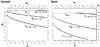 |
Fig. 4 The transfers capable of producing the present orbits of Halimede (left panel) and Nereid (right panel). Lower curve corresponds to the minimum impactor speed vim and an impactor mass mi = 1 m⊕. Intermediate curve corresponds to the maximum impactor speed viM and mi = 1 m⊕. Upper curve corresponds to vim and mi = 3.5 m⊕. The maximum current eccentricity emax is shown by a dotted line. For Halimede the upper curve and emax overlap. A (B) is the square of the ratio of the satellite’s speed just before (after) the impact on the escape velocity at the satellite’s location just before (after) the impact. e1m (e2m) is the minimum eccentricity of the orbits before (after) collision. |
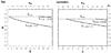 |
Fig. 5 The transfers capable of producing the present orbits of Sao (left panel) and Laomedeia (right panel). Lower curve corresponds to the minimum impactor speed vim and an impactor mass mi = 1 m⊕. Upper curve left panel corresponds to vim and mi = 1.6 m⊕ which is the same as for viM and mi = 1 m⊕. Upper curve right panel corresponds to vim and mi = 1.35 m⊕. There is no transfer for viM and mi = 1 m⊕. The maximum current eccentricity emax is shown by a dotted line. A (B) is the square of the ratio of the satellite’s speed just before (after) the impact on the escape velocity at the satellite’s location just before (after) the impact. e1m (e2m) is the minimum eccentricity of the orbits before (after) collision. |
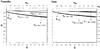 |
Fig. 6 The transfers capable of producing the present orbits of Psamathe (left panel) and Neso (right panel). Lower curve corresponds to the minimum impactor speed vim and an impactor mass mi = 1 m⊕. Intermediate curve corresponds to the maximum impactor speed viM and mi = 1 m⊕. Upper curve left panel corresponds to vim and mi = 2.3 m⊕. Upper curve right panel corresponds to vim and mi = 1.8 m⊕. The maximum current eccentricity emax is shown by a dotted line. In both panels the upper curve and emax overlap. A (B) is the square of the ratio of the satellite’s speed just before (after) the impact on the escape velocity at the satellite’s location just before (after) the impact. e1m (e2m) is the minimum eccentricity of the orbits before (after) collision. |
Using the current orbital elements of the Neptunian irregular satellites as initial conditions (see Table 2), their orbital evolution over a period of 105 yrs is computed using the integrator evorb 13 of Fernández et al. (2002), where the perturbations of the Sun, Jupiter, Saturn and Uranus are included. The minimum, mean, and maximum eccentricities and semiaxes are shown in Table 3 for all the Neptunian irregular satellites with the exception of Triton. We assume that gravitational perturbations are the only effect capable of altering the orbital elements of the irregular satellites during Solar System evolution after the GC since gas drag caused by an ice giant’s envelope proves negligible (Parisi et al. 2008).
We compute a1M and a2M from the upper and lower bounds of ΔV obtained through Eq. (10) using vi = viM and vi = vim, respectively. We take viM = 40 km s-1 and vim from Eq. (3). We take mi = 1 m⊕ as the minimum impactor mass. For each A, we then calculate the values of B(B = B′/(1 + mi/mN)) corresponding to the transfers to a2M = [amax, amin], where amax and amin are the current maximum and minimum semiaxes of the irregular satellites tabulated in Table 3. Introducing these values of B in Eq. (13), we get the minimum possible values of e2min, e2m, that the orbit of each irregular satellite may acquire at impact for each initial condition A.
The transfer of each irregular satellite from its original orbit to the present one is only possible for those values of (A,B) which satisfy the condition e2m < emax (emax tabulated in Table 3). Transfers with A < B, imply that the irregular satellite belongs from an inner orbit, while transfers with A > B imply that the irregular satellite belongs from an outer orbit; i.e., the GC may produce the permanent capture of a body undergoing a temporary capture or even in heliocentric orbit (A ≥ 1).
The transfers of Halimede and Nereid are shown in Fig. 4, those of Sao and Laomedeia in Fig. 5, and the transfers of Neso and Psamathe are displayed in Fig. 6. The lower curve in Figs. 4–6 represents the transfers for vi = vim and mi = 1 m⊕. It should be noted that by minimizing vi and mi, we are maximizing the number of transfers. The real eccentricity that the irregular satellite may acquire for each vi and mi may take any value between e2m and emax. The probability of the existence of the irregular satellite prior to the GC diminishes as e2m approaches emax.
In Fig. 4, the intermediate curve represents the transfers for mi = 1 m⊕ and vi = viM. The transfers for mi = 1 m⊕ and vim ≤ vi ≤ viM fall between the lower and intermediate curves. The upper curve corresponds to vim and mi = 3.5 m⊕, and emax and the upper curve overlap. Halimede and Nereid then set an upper bound on mi of 3.5 m⊕. Within this mass limit, the GC itself could provide a mechanism for the capture of Halimede and Nereid.
In Fig. 5, the transfers for Sao are shown in the left panel. There are no transfers for viM for any impactor mass. The upper curve shows the transfers for vim and mi = 1.6 m⊕, which is very close to emax. There is no transfer for mi ≥ 1.7 m⊕. Sao set an upper bound of 1.7 m⊕ on the impactor mass. The transfers of Laomedeia are displayed in the right panel. The upper curve displays the transfers for vim and mi = 1.35 m⊕, which are the same as for viM and mi = 1 m⊕. Laomedeia set an upper bound on mi of 1.4 m⊕. Within this mass limit, the GC itself could provide a mechanism for the capture of Sao and Laomedeia.
The transfers of Psamathe are shown in the left panel and those of Neso in the right panel of Fig. 6. The intermediate curve corresponds to the transfers for viM and mi = 1 m⊕. The upper curve corresponds to vim and mi = 2.3 m⊕ (Psamathe), and mi = 1.8 m⊕ (Neso). Psamathe set an upper bound on mi of 2.3 m⊕, while Neso of 1.8 m⊕. Within this mass limit, the GC itself could provide a mechanism for the capture of Psamathe and Neso. The transfers of Fig. 6 have been computed over a range of 200 RN around the current orbital semiaxes of both irregular satellites (see Table 3). However, e2m lies close to emax for vi > vim and mi > 1m⊕. This result makes the existence of Neso and Psamathe prior to the GC, as well as their capture by the GC, a possible but not very probable event.
Parisi et al. (2008) carried out a somewhat similar model of the Uranian system. They obtained strong constraints for two Uranian irregular satellites: Prospero and Trinculo. The only transfers for both irregular satellites were close to the pericenter of an eccentric initial orbit (e1m > 0.58 for Prospero and e1m > 0.62 for Trinculo). e2m for Trinculo resulted in the range [0.16–0.23], very close to emax(0.237). Moreover, for Prospero e2m was ~emax(0.571). This result implied that Prospero could not survive stochastic impacts. Either Prospero was created after the epoch of giant impacts or giant impacts did not occur.
In this paper, Laomedeia set an upper constraint on the impactor mass of 1.4 m⊕. Assuming that the Neptunian irregular satellites belong to a common origin, then they set an upper constraint of 1.4 m⊕ on the impactor masses in the trans-Saturnian region at the end of Neptune formation.
Assuming that giant impacts occurred beyond oligarchy, our results imply that either the oligarchic masses in the trasn-Saturnian region at the end of Neptune formation were less that 1.4 m⊕, or the current Neptunian irregular satellites had to be captured after the end of stochastic impacts. Alternatively, parent objects with orbits different to the irregular satellites’ current orbits could have been captured by any process before or during stochastic impacts without restrictions on the impactor mass, but the present population of irregular satellites should then be the result of their later collisional evolution. This possibility would agree with the results of Bottke et al. (2010).
4. Discussion
It has long been known that dynamical times in the trans-Saturnian MMSN are so long that core growth takes more than
15 Myr. Observations of young, solar-type stars suggest that circumstellar disks dissipate on a timescale of few Myr (e.g. Briceño et al. 2001). Different models and scenarios have been proposed to account for the formation of the ice giants within the protoplanetary disk lifetime. Modern models shorten the timescale for giant planet formation if taking a higher initial surface density into account well above that of the MMSN and/or the formation of all giant planets in an inner compact configuration (Dodson-Robinson & Bodenheimer 2010; Benvenuto et al. 2009; Thommes et al. 2003; Tsiganis et al. 2005).
Core accretion models of giant planet formation in situ (Pollack et al. 1996) and core accretion models with the giant planets forming at the initial semiaxes of the Nice model (Dodson-Robinson & Bodenheimer 2010; Benvenuto et al. 2009) compute the solid component because of the accretion of planetesimals. However, no core accretion model has at present, considered the angular momentum transfer during accretion and the possible accretion of other protoplanets onto the core with the exception of Korycansky et al. (1990) who carried out a hydro-dynamical model of a giant impact on Uranus.
Modern scenarios have several difficulties to overcome, and inconsistencies among the different models and scenarios are still present. We discuss four important issues below.
-
1)
Most core accretion models (e.g. Dodson-Robinson &Bodenheimer 2010), assume planetesimals encountering thecore at the Hill velocity; i.e., they do not take the stirring of thesebodies into account. The Hill velocityvH is a characteristic velocity associated with the Hill radius RH and is defined as vH = ΩRH, where Ω is the orbital frequency around the Sun. A speed of the surrounding planetesimals higher than vH would diminish the rate of growth of the ice giants in the massive planetesimals disk: either they had formed in situ or at 10–20 AU.
-
2)
An initial mass 5–10 the MMSN is required to shorten the timescale of ice giants formation, but within a 10 MMSN, Jupiter falls like a stone into the Sun due to type III migration (Crida 2009).
-
3)
If oligarchic masses can reach the isolation mass in 1–10 Myr at 10–30 AU is unknown. The final mass of the oligarchs in the outer solar System remains an open question. Without collisions among oligarchs, the mass of the core of proto-Uranus and proto-Neptune in the frame of the MMSN is the mass of an oligarch; i.e., much low than the present solid cores of Uranus and Neptune (either the ice planets had formed in situ or between 10–20 AU). Collisions among oligarchs takes a very long time to form the ice giants cores. Then, an initial surface density ~5–10 times that of the MMSN would be required to produce oligarchs with masses similar to those of the ice giants cores. However, a solid surface density of this size would lead to the formation of about five ice giants instead of two, which occurred with the other three giants; i.e., whether they were ejected or if they simply were spread out being all retained is a matter of debate (Goldreich et al. 2004; Dodson-Robinson & Bodenheimer 2010; Ford & Chiang 2007; Levison & Morbidelli 2007). In the last case, then, where are they? However, Thommes et al. (2003) have shown that even in a disk 10 times the MMSN, oligarchs do not have time to reach their isolation mass in the outer Solar System, and even an Earth mass at the orbit of Uranus by 10 Myr is implausible.
-
4)
Actually, the mass of the planetesimals from which Uranus and Neptune accreted is a matter of debate. Goldrecih et al. (2004) suggest that, in the dispersion dominate regime the velocity dispersion of small bodies u could exceed their surface escape velocity, and thus collisions at these speeds would be destructive. They speculate that before the oligarchs become planets, small bodies could fragment, reducing their size. Smaller size would imply smaller u, hence faster accretion, thus returning to the case u ≤ vH at isolation. However, there is no reason planetesimals should fragment in the dynamically cold disk required to produce Uranus and Neptune in situ (Dodson-Robinson & Bodenheimer 2010). It is usually believed that the planetesimal distribution follows a power law of the type dn ∝ m − αdm (e.g. Benvenuto et al. 2009, and references therein). Indeed, Jupiter family comets follow a distribution of this type with α = 11/6. Benvenuto et al. (2009) computed the formation of Uranus and Neptune assuming the initial semiaxes distribution of the Nice model taking α = 2.5. They approached the continuous distribution to a discrete distribution with planetesimal sizes in the range 30 m 100 km. However, Dodson-Robinson & Bodenheimer (2010) computed the accretion of Uranus and Neptune in the frame of the Nice model, too, but considered planetesimals with radii of several hundred kilometers since they assumed the theory of planetesimal formation based on the streaming instability which produces planetesimals of about 600 km (Johansen et al. 2007). Although the streaming instability has several benefits, observational evidence (e.g., comet outbursts and chondrules) shows a fractal structure of the planetesimals consistent with coagulation processes for planetesimal formation (Paszun & Dominik 2009). According to Morbidelli et al. (2009), asteroids were born big, suggesting that the minimal size of the planetesimals was ~100 km.
In summary, it is not known whether the ice planets formed in situ, or well inside the 20 UA and/or if the initial mass of the nebula was that of the MMSN or much larger. Moreover, the mass of the planetesimals from which Uranus and Neptune accreted remains a matter of debate. It is necessary to look for independent ways of setting constraints on models of ice giant planet formation.
Our models are independent of unknown parameters, such as the mass and distribution of the planetesimals, the location at which Uranus and Neptune were formed, the Solar Nebula initial surface mass density, and the regime of growth. Our constraints on the oligarchic masses may be used to set constraints on planetary formation scenarios.
5. Conclusions
We have modeled the angular momentum transfer to proto-Neptune and the impulse transfer to its irregular satellites by the last stochastic collision (GC) between the protoplanet and an oligarchic mass. Since stochastic impacts are aleatory and their number is uncertain, the rotational properties of proto-Neptune and the orbital properties of the Neptunian system before the GC are taken as initial free parameters in our model and are constrainted using the present rotational parameters of Neptune and the present orbital and physical properties of Neptune and its irregular satellite population.
Assuming a minimum impactor mass mi ~ 1 m⊕, the mass of the last impactor mi ≤ 4 m⊕ is required to account for the current spin properties of Neptune. This result is invariant: Neptune had formed either in situ or between 10–20 AU and does not depend on the possible occurrence of the stochastic impact during or after migration. A collision with mi > 4 m⊕ could not have occurred since it cannot reproduce the present rotational and physical properties of the planet, unless the impact parameter of the collision was very small. The formation of Neptune as the result, for instance, of collisional accretion between two similar oligarchs with masses ~7 m⊕ seems to be unlikely. Assuming the occurrence of giant impacts as the cause of Neptune’s obliquity, the 4 m⊕ mass limit must be understood as an upper bound for the oligarchic masses in the trans-Saturnian region at the end of Neptune’s formation.
The study of the origin of irregular satellites of giant planets is very important because it puts constraints on formation processes of giant planets and may probe the properties of the primordial planetesimal disk from which irregular satellites were captured. Although recent models study the capture of irregular satellites by close encounters between giant planets in the framework of the Nice model (Bottke et al. 2010), there is very little work on their capture and loss by stochastic collisions (Parisi et al. 2008).
We found that either the mass of the last impactor on Neptune was less than ~1.4 m⊕, or the present Neptunian irregular satellites had to be formed or captured after the end of stochastic impacts. This result is invariant: Neptune had formed either in situ or between 10–20 AU and does not depend on the possible occurrence of the stochastic impacts during or after migration.
If the present population of irregular satellites were captured after the end of stochastic impacts, the mechanism of capture able to operate at such late stages in the scenario of the formation of the planet should be investigated. Alternatively, parent objects with orbits different from the irregular satellites’ current orbits could have been captured by any process before or during stochastic impacts, but the present population of irregular satellites should be the result of their later collisional evolution. This possibility would agree with the results of Bottke et al. (2010).
Colors are an important diagnostic tool in attempting to unveil the physical status and the origin of the Neptunian irregular satellites. In particular it is very important to assess whether it is possible to define subclasses of irregular satellites just by looking at colors and by comparing colors of these bodies with colors of minor bodies in the outer Solar System. The knowledge of the primordial population of irregular satellites could offer valuable clues to know whether Neptune was formed in situ or between 10–20 AU. An intensive search for fainter irregular satellites and a long term program of observations able to recover lightcurves, colors, and phase effects in a “self consistent” manner is mandatory.
In all the cases, vi must be zero for α = 0° and T = T0. However, looking at the figures, the root of Eq. (1) shifts slightly to the left side of T0 = T as mi increases. In the development of Eq. (1), we considered an expression to first order in terms of the protoplanet radius increment for the mass increment mi/mN (Parisi & Brunini 1997). For mi = 1 m⊕, this approximation introduces an error of ~10-3 in computing mi/mN, while for mi = 2.7 m⊕, this error is ~0.02 and ~0.05 for mi = 4 m⊕.
Acknowledgments
M.G.P. research was supported by Intituto Argentino de Radioastronomía, IAR-CONICET, and by CONICET grant PIP 112-200901-00461, Argentina. L.d.V. research was supported by CONICYT Chile and DAS Universidad de Chile.
References
- Agnor, C. B., & Hamilton, D. P. 2006, Nature, 441, 192 [NASA ADS] [CrossRef] [PubMed] [Google Scholar]
- Benvenuto, O. G., Fortier, A., & Brunini, A. 2009, Icarus, 204, 752 [NASA ADS] [CrossRef] [Google Scholar]
- Bodenheimer, P., & Pollack, J. B. 1986, Icarus, 67, 391 [NASA ADS] [CrossRef] [Google Scholar]
- Bottke, W. F., Nesvorny, D., Vokrouhlicky, D., & Morbidelli, A. 2010, AJ, 139, 994 [NASA ADS] [CrossRef] [Google Scholar]
- Boué, G., & Laskar, J. 2010, ApJ, 712, L44 [NASA ADS] [CrossRef] [Google Scholar]
- Briceño, C., Vivas, A. K., Calvet, N., et al. 2001, Science, 291, 93 [NASA ADS] [CrossRef] [Google Scholar]
- Brunini, A. 1995, Earth, Moon, and Planets, 71, 281 [Google Scholar]
- Brunini, A., Parisi, M. G., & Tancredi, G. 2002, Icarus, 159, 166 [NASA ADS] [CrossRef] [Google Scholar]
- Chambers, J. E. 2001, Icarus, 152, 205 [NASA ADS] [CrossRef] [Google Scholar]
- Colombo, G., & Franklin, F. A. 1971, Icarus, 15, 186 [NASA ADS] [CrossRef] [Google Scholar]
- Crida, A. 2009, ApJ, 698, 606 [NASA ADS] [CrossRef] [Google Scholar]
- Cuk, M., & Burns, J. A. 2003, Icarus, 167, 369 [Google Scholar]
- Cuk, M., & Gladman, B. 2005, ApJ, 626, L113 [NASA ADS] [CrossRef] [Google Scholar]
- Dodson-Robinson, S. E., & Bodenheimer, P. 2010, Icarus, 207, 491 [NASA ADS] [CrossRef] [Google Scholar]
- Fernández, J. A., Gallardo, T., & Brunini, A. 2002, Icarus, 159, 358 [NASA ADS] [CrossRef] [Google Scholar]
- Ford, E. B., & Chiang, E. I. 2007, ApJ, 661, 602 [NASA ADS] [CrossRef] [Google Scholar]
- Goldreich, P., Murray, N., Longaretti, P. Y., & Bandfield, D. 1989, Science, 245, 500 [NASA ADS] [CrossRef] [PubMed] [Google Scholar]
- Goldreich, P., Lithwick, Y., & Sari, R. 2004, ARA&A, 42, 549 [NASA ADS] [CrossRef] [Google Scholar]
- Grav, T., Holman, J., Matthew, J., & Fraser Wesley, C. 2004, ApJ, 613, L77 [NASA ADS] [CrossRef] [Google Scholar]
- Greenberg, R. 1974, Icarus, 23, 51 [NASA ADS] [CrossRef] [Google Scholar]
- Hamilton, D. P., & Ward, W. R. 2004, AJ, 128, 2510 [NASA ADS] [CrossRef] [Google Scholar]
- Heppenheimer, T. A., & Porco, C. 1977, Icarus, 30, 385 [NASA ADS] [CrossRef] [Google Scholar]
- Holman, M. J., Kavelaars, J. J., Grav, T., et al. 2004, Nature, 430, 865 [NASA ADS] [CrossRef] [PubMed] [Google Scholar]
- Jewitt, D., & Sheppard, S. 2005, Space Sci. Rev., 116, 441 [Google Scholar]
- Johansen, A., Oishi, J. S., Low, M.-M. M., et al. 2007, Nature, 448, 1022 [Google Scholar]
- Korycansky, D. G., Bodenheimer, P., Cassen, P., & Pollak, J. B. 1990, Icarus, 84, 528 [NASA ADS] [CrossRef] [Google Scholar]
- Kubo-Oka, T., & Nakazawa, K. 1995, Icarus, 114, 21 [NASA ADS] [CrossRef] [Google Scholar]
- Lee, M. H., Peale, S. J., Pfahl, E., & Ward, R. W. 2007, Icarus, 190, 103 [NASA ADS] [CrossRef] [Google Scholar]
- Levison, H. F., & Morbidelli, A. 2007, Icarus, 189, 196 [NASA ADS] [CrossRef] [Google Scholar]
- Levison, H. F., Bottke, W. F., Gounelle, M., et al. 2009, Nature, 460, 364 [NASA ADS] [CrossRef] [PubMed] [Google Scholar]
- Lissauer, J. J., & Kary, D. M. 1991, Icarus, 94, 126 [NASA ADS] [CrossRef] [Google Scholar]
- Lissauer, J. J., & Safronov, V. 1991, Icarus, 93, 288 [NASA ADS] [CrossRef] [Google Scholar]
- Lissauer, J. J., Berman, A. F., Greenzweig, Y., & Kary, D. M. 1997, Icarus, 127, 65 [NASA ADS] [CrossRef] [Google Scholar]
- Maris, M., Carraro, G., Cremonese, G., & Fulle, M. 2001, AJ, 121, 2800 [NASA ADS] [CrossRef] [Google Scholar]
- Maris, M., Carraro, G., & Parisi, M. G. 2007, A&A, 472, 311 [NASA ADS] [CrossRef] [EDP Sciences] [Google Scholar]
- Morbidelli, A., Bottke, W., Nesvorny, D., & Levison, H. G. 2009, Icarus, 204, 558 [NASA ADS] [CrossRef] [Google Scholar]
- Nesvorny, D., Alvarellos, J. L. A., Dones, L., & Levison, H. 2003, AJ, 126, 398 [NASA ADS] [CrossRef] [Google Scholar]
- Nesvorny, D., Beaugé, C., & Dones, L. 2004, AJ, 127, 1768 [NASA ADS] [CrossRef] [Google Scholar]
- Nesvorny, D., Vokrouhlický, D., & Morbidelli, A. 2007, AJ, 133, 1962 [NASA ADS] [CrossRef] [Google Scholar]
- Parisi, M. G., & Brunini, A. 1997, Planet. Space Sci., 45, 181 [NASA ADS] [CrossRef] [Google Scholar]
- Parisi, M. G., Carraro, G., Maris, M., & Brunini, A. 2008, A&A, 482, 657 [NASA ADS] [CrossRef] [EDP Sciences] [Google Scholar]
- Paszun, D., & Dominik, C. 2009, A&A, 507, 1023 [NASA ADS] [CrossRef] [EDP Sciences] [Google Scholar]
- Pollack, J. B., Burns, J. A., & Tauber, M. E. 1979, Icarus, 37, 587 [NASA ADS] [CrossRef] [Google Scholar]
- Pollack, J. B., Hubickyj, O., Bodenheimer, P., et al. 1996, Icarus, 124, 62 [NASA ADS] [CrossRef] [Google Scholar]
- Schlichting, H. E., & Sari, R. 2007, AJ, 658, 593 [Google Scholar]
- Sheppard, S. S., Jewitt, D. C., & Kleyna, J. 2006b, AJ, 132, 171 [NASA ADS] [CrossRef] [Google Scholar]
- Thommes, E. W., Duncan, M. J., & Levison, H. F. 2003, Icarus, 161, 431 [NASA ADS] [CrossRef] [MathSciNet] [Google Scholar]
- Tremaine, S. 1991, Icarus, 89, 85 [NASA ADS] [CrossRef] [Google Scholar]
- Tsiganis, K., Gomes, R., Morbidelli, A., & Levison, H. F. 2005, Nature, 435, 459 [NASA ADS] [CrossRef] [PubMed] [Google Scholar]
- Tsui, K. H. 1999, Planet. Space Sci., 47, 917 [Google Scholar]
- Vokrouhlicky, D., Nesvorny, D., & Levison, H. F. 2008, AJ, 136, 1476 [NASA ADS] [Google Scholar]
All Tables
Orbital and physical parameters of the Neptunian irregulars taken from JPL (http://ssd.jpl.nasa.gov).
Variation in the orbital eccentricity and semiaxis (in units of RN = 24 764 km) of the Neptunian irregulars due to Solar and giant planet perturbations over a period of 105 yrs. Δamin = amean − amin and Δamax = amax − amean.
All Figures
|
Fig. 1 Impactor incident speed vi as a function of the initial period T0 for mi = 1 m⊕, obtained through angular momentum transfer for the most probable impact parameter b = 2/3 Rc. a) α = 0°, b) α = 29.58°, c) α = 60°, d α = 90°, e) α = 130°, and f) α = 170°. The upper constraint on vi (viM) is depicted by dotted lines while the lower constraint on vi (vim) is shown by dashed lines. viM and vim are obtained from simple dynamical constraints. |
| In the text | |
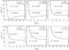 |
Fig. 2 The same as in Fig. 1 for mi = 2.7 m⊕. |
| In the text | |
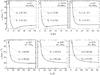 |
Fig. 3 The same as in Fig. 1 for mi = 4 m⊕. |
| In the text | |
|
Fig. 4 The transfers capable of producing the present orbits of Halimede (left panel) and Nereid (right panel). Lower curve corresponds to the minimum impactor speed vim and an impactor mass mi = 1 m⊕. Intermediate curve corresponds to the maximum impactor speed viM and mi = 1 m⊕. Upper curve corresponds to vim and mi = 3.5 m⊕. The maximum current eccentricity emax is shown by a dotted line. For Halimede the upper curve and emax overlap. A (B) is the square of the ratio of the satellite’s speed just before (after) the impact on the escape velocity at the satellite’s location just before (after) the impact. e1m (e2m) is the minimum eccentricity of the orbits before (after) collision. |
| In the text | |
|
Fig. 5 The transfers capable of producing the present orbits of Sao (left panel) and Laomedeia (right panel). Lower curve corresponds to the minimum impactor speed vim and an impactor mass mi = 1 m⊕. Upper curve left panel corresponds to vim and mi = 1.6 m⊕ which is the same as for viM and mi = 1 m⊕. Upper curve right panel corresponds to vim and mi = 1.35 m⊕. There is no transfer for viM and mi = 1 m⊕. The maximum current eccentricity emax is shown by a dotted line. A (B) is the square of the ratio of the satellite’s speed just before (after) the impact on the escape velocity at the satellite’s location just before (after) the impact. e1m (e2m) is the minimum eccentricity of the orbits before (after) collision. |
| In the text | |
|
Fig. 6 The transfers capable of producing the present orbits of Psamathe (left panel) and Neso (right panel). Lower curve corresponds to the minimum impactor speed vim and an impactor mass mi = 1 m⊕. Intermediate curve corresponds to the maximum impactor speed viM and mi = 1 m⊕. Upper curve left panel corresponds to vim and mi = 2.3 m⊕. Upper curve right panel corresponds to vim and mi = 1.8 m⊕. The maximum current eccentricity emax is shown by a dotted line. In both panels the upper curve and emax overlap. A (B) is the square of the ratio of the satellite’s speed just before (after) the impact on the escape velocity at the satellite’s location just before (after) the impact. e1m (e2m) is the minimum eccentricity of the orbits before (after) collision. |
| In the text | |
Current usage metrics show cumulative count of Article Views (full-text article views including HTML views, PDF and ePub downloads, according to the available data) and Abstracts Views on Vision4Press platform.
Data correspond to usage on the plateform after 2015. The current usage metrics is available 48-96 hours after online publication and is updated daily on week days.
Initial download of the metrics may take a while.