| Issue |
A&A
Volume 530, June 2011
|
|
|---|---|---|
| Article Number | A125 | |
| Number of page(s) | 13 | |
| Section | Extragalactic astronomy | |
| DOI | https://doi.org/10.1051/0004-6361/201016198 | |
| Published online | 24 May 2011 | |
A comprehensive approach to analyzing the XMM-Newton data of Seyfert 1 galaxies
1
Universidad Autónoma de Madrid, Ctra. de Colmenar Km.15, Cantoblanco,
28049
Madrid, Spain
e-mail: This email address is being protected from spambots. You need JavaScript enabled to view it.
2
XMM-Newton Science Operations Center, ESAC, ESA,
POB 78, 28691
Villanueva de la Cañada,
Madrid,
Spain
3
Facultad de Cs. Astronómicas y Geofísicas, Universidad Nacional de
La Plata, Paseo del Bosque
s/n, 1900
La Plata,
Argentina
4
Instituto de Astronomía, Universidad Nacional Autónoma de
México, Apartado Postal
70-264, 04510
México DF,
México
Received: 24 November 2010
Accepted: 15 March 2011
Abstract
Aims. We seek a comprehensive analysis of all the information provided by the XMM-Newton satellite of the four Seyfert 1 galaxies ESO 359-G19, HE 1143-1810, CTS A08.12, and Mrk 110, including the UV range, to characterize the different components that are emitting and absorbing radiation in the vicinity of the active nucleus.
Methods. The continuum emission was studied through the EPIC spectra by taking advantage of the spectral range of these cameras. The high-resolution RGS spectra were analyzed to characterize the absorbing and emission line features that arise in the spectra of the sources. All these data, complemented by information in the UV, are analyzed jointly in order to achieve a consistent characterization of the observed features in each object.
Results. The continuum emission of the sources can be characterized either by a combination of a power law and a black body for the weakest objects or by two power law components for the brightest ones. The continuum is not absorbed by neutral or ionized material in the line of sight to any of these sources. In all of them we have identified a narrow Fe-Kα line at 6.4 keV. In ESO 359-G19 we also find an Fexxvi line at about 7 keV. In the soft X-rays band, we identify only one Ovii line in the spectra of HE 1143-1810 and CTS A08.12, and two Ovii-Heα triplets and a narrow Oviii-Lyα emission line in Mrk 110.
Conclusions. Not detecting warm material in the line of sight to the low state objects is due to intrinsically weaker or absent absorption in the line of sight and not to a low signal-to-noise ratio in the data. Besides this, the absence of clear emission lines cannot be fully attributed to dilution of those lines by a strong continuum.
Key words: galaxies: active / galaxies: Seyfert / galaxies: general / X-rays: galaxies
CONICET, Argentina.
© ESO, 2011
1. Introduction
The spectral features characteristic of the X-ray spectra of active galactic nuclei (AGNs) are conspicous signatures of the physical processes taking place in the inner regions of these objects, and analyzing them has significantly improved our understanding of these issues in the last few years of the 20th century. However, it has also become evident that a much better understanding is needed, and in fact it can be achieved by detailed analysis of the data acquired with the present generation of X-ray telescopes.
In this paper we present a comprehensive analysis of all the available data obtained with the XMM-Newton satellite of four Seyfert 1 galaxies: ESO 359-G19, HE 1143-1810, CTS A08.12, and Mrk 110 in order to try to characterize the different components of the gas that imprint the absorption and emission features in the X-ray spectra of these objects. The low-resolution and large spectral range EPIC (European Photon Image Camera) spectra were used to study the continuum emission. The high-resolution RGS (Reflection Grating Spectrometer) spectra are analyzed to search for and characterize, if found, the absorbing and emission line features that arise in the spectra of these sources.
General characteristics of the objects selected for our study.
The first of our objects, ESO 359-G19, has been classified as a Seyfert 1 galaxy by Maza et al. (1992) using longslit spectrophotometric data. It has not been studied in detail in spite of being observed on many occasions (Fairall 1988; Wisotzki et al. 1996; Karachentsev & Makarov 1996). It was previously observed in X-rays with the ROSAT (1990 August; Voges et al. 1999; Thomas et al. 1998) and Einstein (Elvis et al. 1992) satellites, as part of the study of the general properties of objects with X-ray emission (Simcoe et al. 1997; Grupe et al. 2001; Jahnke & Wisotzki 2003; Fuhrmeister & Schmitt 2003). More recently, it has been observed by Swift (2008 October) as part of a sample of 92 bright soft X-ray selected AGNs (Grupe et al. 2010).
HE 1143-1810 was classified as a type 1 Seyfert AGN by Remillard et al. (1986). These authors also found that this galaxy has a companion object, LEDA 867889, which shows neither signatures of nuclear activity nor the characteristic emission of Hii galaxies. It is located at about 20 kpc from HE 1143-1810. From extreme UV observations with FUSE, Wakker et al. (2003) studied the gas surrounding the AGN and concluded that the positive-velocity Ovi absorption extends much further than expected for a Galactic origin, although they did not find a clear separation between an intrinsic Ovi line and the Galactic absorption. The authors separated the thick disk and high-velocity cloud components at a velocity of 100 km s-1. However, using the same and newer observations from FUSE, Dunn et al. (2007) could not identify any intrinsic absorption feature in this galaxy.
Very little is known in detail about CTS A08.12, despite its being included in a large number of statistical studies at different wavelengths (e.g. Voges et al. 1999; Bauer et al. 2000; Ebisawa et al. 2003; Verrecchia et al. 2007; Mauch & Sadler 2007). It was classified as a Seyfert 1 by Maza et al. (1994).
Finally, Mrk 110 is a nearby Seyfert 1 galaxy with a very irregular morphology (Bischoff & Kollatschny 1999), which may indicate that it has suffered some kind of interaction with a companion galaxy (Hutchings & Craven 1988). From optical spectroscopy covering a narrow spectral range, between 4300 and 5700 Å, Boroson & Green (1992) estimated a full width at half maximum (FWHM) of 2120 km s-1 for the Hβ emission line, and observed a very broad Hei 4471 Å emission line. More recently, Grupe et al. (2010) have derived a FWHM of 1760 ± 50 km s-1 for Hβ, less than the value used as one of the criteria to distinguish Narrow Line Seyfert 1 (NLS1) from Seyfert 1 galaxies. Nevertheless, the objects was classified as a NLS1 by Véron-Cetty & Véron (2006). As in the case of UGC 11763 (Cardaci et al. 2009), Mrk 110 seems to be located in a transition zone between the Seyfert 1 and NLS1 classifications, showing some of the properties of each class.
In Table 1 we list the general characteristics of the galaxies in our sample as obtained from the literature: celestial coordinates (α2000 and δ2000), redshifts (z), the distances in Mpc as derived from their redshifts using the expression D = (cz/H0) and adopting H0 = 75 km s-1 Mpc-1, and estimated Galactic hydrogen column densities (NH) in the line of sights taken from Dickey & Lockman (1990).
The paper is organized as follows. In Sect. 2 we describe the observations and data reduction. The optical-UV results and the X-ray spectral analysis are presented in Sects. 3 and 5, respectively. In Sect. 4 we analyze the variability during the XMM-Newton observation and compare our observed fluxes with those from the literature. Our results are discussed in Sect. 6. And finally, the summary and conclusions of this work are given in Sect. 7.
2. Observations
ESO 359-G19, HE 1143-1810, CTS A08.12, and Mrk 110 were observed by XMM-Newton (Jansen et al. 2001) in 2004 (Table 2) as part of a project to characterize the complex profile of the iron Kα line and the features that sometimes appear in the soft X-ray spectral range. The four galaxies of this study were selected to be brighter than 0.85 c s-1 in the ROSAT Bright Source Catalog (Voges et al. 1999) and not previously observed by the XMM-Newton. Exposure times were estimated from the available ASCA and ROSAT observations. The observing modes for EPIC-pn and EPIC-MOS1 (Turner et al. 2001) were selected according to the expected count rates (from PIMMS1) to avoid pile-up effects, and the selections are listed in Table 3. EPIC-MOS2 camera was always set in full frame mode to allow cross check for bright serendipitous X-ray sources in the field that could contaminate the RGS spectra. RGSs (den Herder et al. 2001) were run in the default spectroscopy mode. Optical Monitor (OM, Mason et al. 2001) observations that combined broad-band imaging filters were requested to investigate the circumnuclear structure in the UV domain with a series of UV-Grism exposures to obtain UV spectral and variability information about the active nucleus.
The OM, when used with broad-band filters, was always operated with the “science user
defined” windows mode. The OM windows were centered on the target, with no spatial binning
to maximize the resolution and with the maximum allowed size for those windows that is
5 1 × 50.
This mode is the best choice for galaxies that are small enough to be fully included in a
few arcmin square window. The default OM windows are designed to provide data over the whole
OM field of view which, because it is larger, needs more time to be fully covered. The
default grism window was selected for using the OM with the UV grism. This window contains
the zeroth-order image and the first-order spectrum of the target at full detector
resolution. More details on the EPIC and OM operating modes can be found in the XMM-Newton Users Handbook (2010).
1 × 50.
This mode is the best choice for galaxies that are small enough to be fully included in a
few arcmin square window. The default OM windows are designed to provide data over the whole
OM field of view which, because it is larger, needs more time to be fully covered. The
default grism window was selected for using the OM with the UV grism. This window contains
the zeroth-order image and the first-order spectrum of the target at full detector
resolution. More details on the EPIC and OM operating modes can be found in the XMM-Newton Users Handbook (2010).
Journal of observations.
Details of XMM-Newton instrument exposures.
The data were processed with the 8.0.0 version of the Science Analysis Subsystem (SAS) software package (Jansen et al. 2001) using the calibration files available in January 2009. All the standard procedures and screening criteria were followed for extracting the scientific products.
2.1. Selection of low background intervals
High background time intervals have been excluded using the method that maximizes the signal-to-noise in the spectrum (MaxSNR) as described in Piconcelli et al. (2004). The observations of ESO 359-G19 and CTS A08.12 were affected by an increase in the background radiation towards the end of the observation. The periods affected by high radiation were not taken into account for the EPIC-MOS spectral extraction. There was no need, however, to reject any time interval from the EPIC-pn data of any of either source. For ESO 359-G19, time intervals with background count rates higher than 0.6 and 3.2 c s-1 had to be discarded from the EPIC-MOS1 and EPIC-MOS2 spectra, respectively. The total discarded time was about 5% for EPIC-MOS1 and about 1.5% for EPIC-MOS2 of the total observing time. In the case of CTS A08.12, time intervals with background count rates higher than 0.9 and 0.5 c s-1 were subtracted of EPIC-MOS1 and EPIC-MOS2, respectively. The total discarded time was about 2.5% and much less than the 1% of the total observing time for EPIC-MOS1 and EPIC-MOS2, respectively.
No high background intervals occurred during the HE 1143-1810 and Mrk 110 observations. Therefore, the EPIC-pn spectrum of HE 1143-1810 and all the EPIC spectra of Mrk 110 did not need to be cut in time. Nevertheless, as a result of applying the MaxSNR procedure, time intervals with background count rates higher than 0.4 c s-1 had to be discarded from both EPIC-MOS spectra of HE 1143-1810. The total discarded time was about 1.5% of the total observing time in each case.
The light curves of the RGS background radiation corresponding to our data show a significant increase towards the end of the ESO 359-G19 observation, reaching even >1 c s-1 for RGS2, whose sensitivity is slightly greater than that of RGS1. Aproximately the first 19 ks of the observation had a background count rate below 0.2 c s-1, and then it increased (in average) to about 0.4 c s-1. During the observations of HE 1143-1810 and Mrk 110, the background count rates of the RGS spectra were less than 0.2 c s-1. Despite the increase in the background radiation that occurred during the ESO 359-G19 and CTS A08.12 observations, it was unnecessary to exclude the periods of increased background radiation since it always remained between 0.1 and 1.3 counts per second, which is considered normal (XMM-Newton SAS Users Guide 2004).
Detailed instruments configurations are given in Table 3 for each object. The last column of this table lists the final effective exposure time after taking the live time2 into account.
3. Optical-UV analysis
OM data were processed with the SAS task omichain and default parameters. In the broad-band OM images, there is no clear evidence of extended emission. The images provide flux measures in the selected filters: B,U, UVW1, UVM2, and UVW2 for all objects and also V for CTS A08.12 and Mrk 110. Table 4 shows the effective wavelengths of these filters, together with measured fluxes. When more than one exposure per filter is available, the mean value is listed. The flux differences on each series of consecutive exposures with the same filter are all compatible with no variability within the measurement errors (<3%).
The spectrum recorded in each individual UV-grism exposure is very weak; in addition, a number of zero-order images near the spectrum location and along the dispersion further complicate the extraction of the source spectrum. As a result, the total signal-to-noise of the extracted spectra was not as high as expected.
Fluxes in the OM filters obtained using aperture photometry.
HE 1143-1810 was observed by the International Ultraviolet Explorer (IUE) in three different epochs between 1987 and 1990 with its Short Wavelength (1150–1950 Å) and Long Wavelength (1950–3200 Å) spectrographs. OM flux measurements in the UVW2, UVM2, and UVW1 filters are overplotted in the top panel of Fig. 1 on the average IUE spectra of each epoch. In this figure we see that the average UV spectrum taken in 1990 is indeed an acceptable representation of the UV spectral energy distribution (SED) of HE 1143-1810 at the time of the XMM-Newton observation. From the IUE average spectrum in the rest frame we took the UV flux at 2500 Å, F(2500 Å) = 2.2 × 10⁻¹⁴ erg cm-2 s-1 Å-1. This value has been corrected for neither the Balmer continuum nor the Feii contributions.
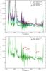 |
Fig. 1 Average IUE spectra (1200–3200 Å) of HE 1143-1810 (top) for the three observing epochs, and Mrk 110 (bottom) for the observing epoch. Solid red circles show the OM measures for the UVW2, UVM2, and UVW1 filters. |
Mrk 110 was also observed by the IUE in 1988 with its Short Wavelength and Long Wavelength spectrographs. Figure 1 (bottom panel) shows the average IUE spectrum with the fluxes obtained from the OM filters overplotted. This figure shows that Mrk 110 was in a lower flux state when observed by IUE than when observed by XMM-Newton. After comparing the fluxes obtained for the OM filters UVM2 and UVW1 with those from the IUE observation for the same wavelengths, we estimated that the difference between them is about 1 × 10-14 erg cm-2 s-1 Å-1. Adding this value to the flux at 2500 Å obtained from the IUE average spectrum in the rest frame and assuming that the shape of the UV continuum is essentially the same for the different epochs (as in the case of HE 1143-1810), we estimate that F(2500 Å) = 2.05 × 10⁻¹⁴ erg cm-2 s-1 Å-1 at the time of our observation.
4. Variability
We analyzed the EPIC-pn soft (0.5–1 keV) and hard (2–10 keV) X-ray background-subtracted
light curves to investigate the variability of the four observed sources during their
XMM-Newton observations. The overall behavior of the light curves of
ESO 359-G19 and CTS A08.12 seems to show a constant average flux value and short-time,
low-amplitude flux variations. In the case of the ESO 359-G19 light curves (upper panel of
Fig. 2), the ratio between the maximum and minimum
count rates is  and
and  for the soft and hard bands, respectively,
thereby indicating no statistically significant variations.
for the soft and hard bands, respectively,
thereby indicating no statistically significant variations.
For CTS A08.12 light curves (lower panel of Fig. 2), the ratios of the maximum to minimum rate are 1.3 ± 0.1 and 1.4 ± 0.2 for soft and hard bands, respectively. Therefore, taking the typical flux variations of this kind of objects into account, the flux variation during the observation was of small amplitude although significant (3σ) in the soft band, and only marginally significant (2σ) in the hard band. Under a careful visual inspection of the light curves, there seems to be an anti-correlation between the variations in the soft and hard light curves: an increment in flux in the soft band seems to correspond to a decrement in the hard band flux, and viceversa. The cross-correlation function between these curves does not suggest that this behavior could be explained by a temporal delay. The soft vs. hard count rates representation shows a weak negative regression that could indicate an anti-correlation. However, there is a large dispersion in the data, so we cannot assert the presence of that anti-correlation based only on the present observations.
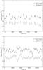 |
Fig. 2 Soft (filled circles) and hard (open squares) EPIC-pn light curves of ESO 359-G19 (upper panel) and CTS A08.12 (lower panel) binned by 1000 s. |
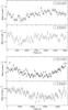 |
Fig. 3 Soft (filled circles) and hard (open squares) EPIC-pn light curves of HE 1143-1810 (upper panel) and Mrk 110 (lower panel) binned by 500 s. |
The light curves of HE 1143-1810 and Mrk 110 are not well modeled by a constant flux function. In the case of HE 1143-1810 the ratios between the maximum and minimum count rates are 1.10 ± 0.04 and 1.18 ± 0.07, indicating that the flux variations are small but significant at the ~2.5σ level (Fig. 3, upper panel). Flux variations in the two bands are well correlated without any temporal delay. For Mrk 110 the ratio between the maximum and minimum count rates for the soft and hard light curves (1.16 ± 0.04 and 1.23 ± 0.07) indicates that the amplitudes of the flux variations are small but significant at 4σ and 3σ levels, respectively (Fig. 3, lower panel). In this case, there is a time lag of about 1000 s between the flux variations in the soft and hard bands, indicating that variations are seen first in the soft band and about 17 min later in the hard band.
Comparison between X-ray fluxes from the literature and from this work.
The X-ray fluxes available from the literature for these objects are summarized in Table 5. For this table we have taken the fluxes listed as Flux1 in the ROSAT All-Sky Bright Source Catalog (Voges et al. 1999) since it is obtained assuming a power law model (αx = 1.3) with an absorbed column density fixed at the Galactic value. Fitting also an absorbed power law to the same ROSAT All-Sky Survey (RASS) data of ESO 359-G19 and Mrk 110, Grupe et al. (2004) found very different flux values (lower than those in Voges et al. 1999, by factors of about 2.2 and 1.7, respectively) in almost the same interval. All these objects show a variation of large amplitude in its soft X-ray flux, from a factor of about 2 for HE 1143-1810 to a factor of about 18 for ESO 359-G19. Fluxes in the 0.1–2.4 keV range taken from ROSAT observations 14 years before the XMM-Newton ones, are found to be larger than measured by us by about one order of magnitude for ESO 359-G19 and CTS A08.12 and by only a factor of 2 for HE 1143-1810. However, in the case of Mrk 110, our estimation of this flux is larger than the one obtained from ROSAT by a factor of 1.7. For this object the maximum soft X-ray flux reported in the literature was measured one year later (1991), also with ROSAT, and is a factor ~1.6 higher than our XMM-Newton value.
Swift observations exist for ESO 359-G19, HE 1143-1810, and Mrk 110. For the first, similar values to those derived by us are reported. In the case of HE 1143-1810 and Mrk 110 our results are higher and lower than those derived from the Swift data by factors of 2.5 and 1.5, respectively. Mrk 110 shows very similar flux values between the data acquired in 1991 and 2010 by ROSAT and Swift, respectively.
In the 2–10 keV range the amplitude of the flux variations is larger than a factor of 2 for HE 1143-1810 and 3.8 for CTS A08.12. For ESO 359-G19 there are no published data in this spectral range, and the hard XMM-Newton (2004) and ASCA (1998) values for Mrk 110are very similar, although the ASCA soft flux is a factor ~1.4 lower than the soft XMM-Newton flux. Unfortunately, for the galaxies studied here there is no data in the hard spectral range taken contemporaneously to the observed highest soft X-ray flux. Taking the fluxes in Table 5 into account for these objects, it becomes clear that, when they were observed by the XMM-Newton satellite, only CTS A08.12 was in the lowest reported activity state, ESO 359-G19 was almost in the lowest reported state (very similar to Swift observations), and HE 1143-1810 and Mrk 110 were in an intermediate state.
5. X-ray spectral analysis
All the EPIC data were checked for no pile-up effects using the SAS task epatplot. We have found these effects to be present in the EPIC-MOS1 and EPIC-MOS2 spectra of HE 1143-1810 and Mrk 110. For these objects we excised the core of the source (i.e., the core of the point spread function) using an annular shape for the source extraction region of the MOS data. The inner radii were selected as the minimum radii that ensures a negligible fraction (less than 5%) of pile-up in the data. The EPIC spectra were extracted using standard parameters. Except for those data affected by pile-up, the source extraction areas were circular regions. All the EPIC spectra were binned to have at least 30 counts per bin.
The RGS data were processed with default parameters except that we discarded potentially problematic cold pixels. All the RGS spectra were binned, losing spectral resolution but increasing the signal-to-noise ratio. We selected a geometrical binning since this method minimizes any smoothing of the absorption and emission features. We binned the RGS data of ESO 359-G19, HE 1143-1810, and CTS A08.12 using 15 channels per bin, while 10 channels per bin were used in the case of Mrk 110. Because the default RGS spectral bin size is 10 mÅ at 15 Å, our final spectra for ESO 359-G19, HE 1143-1810, and CTS A08.12 have bins of about 150 mÅ at that wavelength, while those of Mrk 110 have bins of about 100 mÅ.
All spectra were fitted using Sherpa package of CIAO 3.4 (Freeman et al. 2001; Silva & Doxsey 2006). We used the χ2 statistics with the Gehrels variance function (Gehrels 1986) and the Powell optimization method, the first because it is based on Poisson statistics for a small number of counts in a bin and on Binomial statistics otherwise, and the second because it is a robust direction-set method for finding the nearby fit-statistical minimum.
Best-fit model to the continuum of the EPIC spectra in the 0.35–10 keV range.
5.1. Low-resolution spectra
For each source we start by fitting only the EPIC-pn spectrum in the hard band (2.0–10.0 keV), then we check for soft excess extending the hard band model to the soft band, and finally we fit the three EPIC (pn, MOS 1 and MOS 2) spectra simultaneously in the whole range considered (0.35–10 keV). Below 1 keV, all the objects analyzed in this work show an X-rays excess over the extrapolation of the harder power law flux. Soft excess components are modeled in the simplest way. We first use a black body component, and in the case this model does not represent the observed excess, we use a power law. Because the Galactic absorption has to be taken into account, we include, in all the source models mentioned from here on, a component that models the Galactic neutral absorption with the hydrogen column density (NH) fixed to the values listed in Table 1. In Table 6 we list – for each source – the best-fit model continuum parameters found by performing the simultaneous EPIC fit.
The criteria we have used to include Gaussian profiles in the models is the same as described in Cardaci et al. (2009). The lines are added constraining their energies to vary in a small range around their laboratory energies (Elab) and taking the redshift of the source into account. Since we cannot use only the F-test as a reliable criterion to compute the statistical significance of a Gaussian line (Protassov et al. 2002), we use a combined method to decide whether to include a line in our final model. Along with the F-test, for which the minimum significance level considered is 95%, we check that the residuals of the new fit at the position of the tested line is less than 1 sigma, and finally we also ensure that the wavelength positioning of the line be consistent with its laboratory wavelength (taking the galaxy redshift into account).
Except for Mrk 110, we find that the fluorescent Fe-Kα emission line is significant to the fit (with more than 99% significance). The Fe-Kα line widths, σ, are small enough to be considered equal to the instrumental resolution.
After analyzing the residuals of the ESO 359-G19 fit, we find a second narrow line at about 7 keV that could be originated by Fexxvi (Elab = 6.966 keV). The line width has been fixed to the instrumental resolution. This line is statistically significant to the fit (with more than 95% significance).
In the residuals of the HE 1143-1810 fit, we see a wide 4σ Gaussian
shape excess between 0.4 and 0.8 keV. This excess is well described with a Gaussian line
centered at  keV (~21.4 Å) with a dispersion of
 keV
(
keV
( km s-1). It could be
interpreted as a blend of Ovii lines.
km s-1). It could be
interpreted as a blend of Ovii lines.
On the CTS A08.12 fit, there is still a small (2 sigma) line-like residual around 6 keV that might indicate a relativistic shape for the Fe-Kα line. Unfortunately, the signal-to-noise ratio of this line is low, and with these data we cannot test the hypothesis of a potential relativistic shape of the Fe-Kα line any further.
In the case of Mrk 110, although there are residuals around 6 keV that could be interpreted as signatures of an Fe-Kα emission line, including this component (with only 70% significance) proved not to be significant to the fit. After the modeling of the soft excess component still remains a broad excess in the residuals between 0.5 and 0.6 keV. We included three Gaussian components at the energy position of the Ovii triplet emission lines (0.5740, 0.5686, 0.5610 keV) to model it. These lines were included with the relative energies between them fixed to the theoretical values, and having the same dispersion. Since the normalizations of two of the lines take lower values (around 2 × 10⁻⁵ and 3 × 10⁻⁶ ph cm-2 s-1) than the third line (about 4 × 10⁻⁴ ph cm-2 s-1) this triplet is dominated by only one component.
The parameter values of the final EPIC model of each object are listed in Tables 6 and 7.
Line parameters included in the best-fit model to the simultaneous three EPIC spectra in the 0.35–10 keV range.
5.2. High-resolution X-ray spectra
The EPIC spectra, with their broad energy coverage provide a good picture of the shape of the continuum emission of the source and its wide emission features. However, the search for narrow features requires using the higher resolution spectra provided by the RGS instruments. On the other hand, by fitting only the RGS spectra, one could find solutions not completely compatible with those derived from the analysis of the EPIC spectra alone. Therefore a comprehensive five-spectra fit including the three EPIC and the two RGS spectra has been made. The EPIC-pn and EPIC-MOS data are restricted to the 0.35–10 keV energy range, while the RGS data are taken in the 0.41 and 1.8 keV (about 6.9–30.2 Å) range.
The best-fitting model obtained using the low-resolution spectra is used as the first approximation for the five-spectra fit. No relevant intrinsic neutral absorption components associated with the studied sources have been found.
For the fit of ESO 359-G19 data we find a model with a hard power law
( ) slightly steeper than for the simple EPIC
fit and with a lower black body temperature (
) slightly steeper than for the simple EPIC
fit and with a lower black body temperature ( ). The parameter values of the Fe lines
identified on the EPIC spectra remain unchanged. In the residuals of the RGS fit
(Fig. 4), we notice a wide feature located at about
20 Å. We tried to model it with a Gaussian component but we did not find a satisfactory
solution. The best-fitting model is plotted in Fig. 4.
). The parameter values of the Fe lines
identified on the EPIC spectra remain unchanged. In the residuals of the RGS fit
(Fig. 4), we notice a wide feature located at about
20 Å. We tried to model it with a Gaussian component but we did not find a satisfactory
solution. The best-fitting model is plotted in Fig. 4.
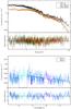 |
Fig. 4 ESO 359-G19. Upper panel: low-resolution X-ray spectra – in the rest frame – as obtained with the EPIC-pn (black dots), EPIC-MOS1 (green diamonds), and EPIC-MOS2 (red squares) cameras. The best-fit model after a comprehensive fit of the EPIC-pn, EPIC-MOS, and RGS spectra (Tables 8 and 9) convolved with the instrument response of each camera is shown as a solid line. Lower panel: high-resolution X-ray spectra – in the rest frame – as obtained with the RGS1 (blue up triangles), and RGS2 (cyan down triangles), and binned to 15 channels per bin. Solid lines are the convolution of the best-fit model after a comprehensive fit of the EPIC-pn, EPIC-MOS, and RGS spectra (Tables 8 and 9) with instrument responses. |
For HE 1143-1810, the same model that fits the EPIC-pn and EPIC-MOS data is also valid
for describing the RGS data in the comprehensive fit
( /d.o.f. = 0.92/2097). When substituting the
broad oxygen line by three lines to account for the Ovii triplet, we find that
the EPIC spectra are not well modeled at soft energies. Residuals show about
4σ departures from zero. We also tested for the presence of narrow
Ovii triplet lines including them only in the RGS spectra model but no
satisfactory solution was found. Figure 5 shows the
model and errors, together with the spectral data.
/d.o.f. = 0.92/2097). When substituting the
broad oxygen line by three lines to account for the Ovii triplet, we find that
the EPIC spectra are not well modeled at soft energies. Residuals show about
4σ departures from zero. We also tested for the presence of narrow
Ovii triplet lines including them only in the RGS spectra model but no
satisfactory solution was found. Figure 5 shows the
model and errors, together with the spectral data.
Also in the case of CTS A08.12, the same model provides a good fit to both the EPIC and the RGS data However, the residuals in the high-resolution spectra fit indicate the need to introduce narrow Gaussian lines at the theoretical wavelengths of the Ovii and Oviii lines. Only one of the Ovii lines is found (the normalizations of the other two are lower than 10-9 ph cm-2 s-1 keV-1), and it is significant to the fit (more than 99% confidence level). The Oviii emission line is not statistically significant to the fit. In this object, the wide feature in absorption that arises between 15 and 17 Å could be the signature of partially ionized material absorbing the source radiation. We tested for the possible presence of such a component using the PHASE photoionization code (Krongold et al. 2003) and find a hydrogen column density lower than 1020 cm-3 for the absorbing gas. Such a component does not affect the X-ray bands analyzed in the present work. The best-fitting model is plotted in Fig. 6.
Continuum parameters of the comprehensive EPIC-pn, EPIC-MOS, and RGS best-fit model for ESO 359-G19, HE 1143-1810, CTS A08.12, and Mrk 110.
Line parameters included in the comprehensive EPIC-pn, EPIC-MOS, and RGS best-fit model for ESO 359-G19, HE 1143-1810, CTS A08.12, and Mrk 110.
The model that best reproduces the EPIC spectra of Mrk 110 leaves residuals on the RSG spectra that could come from the presence of narrow emission lines. Also departures 2σ larger than zero are found at ~6.4 keV that point to the presence of a weak Fe line. Although the addition of this line was found to not be statistically significant to the fit of the EPIC data, we decided to incorporate it in the five-spectra fit. This line was modeled with a Gaussian profile whose width was left free. As a result, a very broad feature (σ ~ 2 keV) centered on ~5 keV was obtained. Since the feature seen in the residuals is not very wide, we tried to find the best parameters for this line “by hand”. Then we realized that the line dispersion could be frozen to the instrumental resolution. With the initial parameters found in this way we get a satisfactory fitting for this Fe emission line at about 6.4 keV, although the fitting process is not able to find the errors associated with the energy value of the line. The narrow features that appear in the RGS data were modeled with a second Ovii triplet (i.e., another set of three Gaussian lines linked in energies and dispersions) and an Oviii line. It should be emphazised that these lines were included only in the RGS model and that all of them turn out to be significant to the fit. Figure 7 shows the final model adopted for Mrk 110, along with the corresponding errors.
The parameter values of the best-fitting model for each of these objects are listed in Tables 8 and 9.
6. Discussion
UV emission
From the OM data of HE 1143-1810 we have found that the IUE average spectrum obtained in 1990 is representative of its flux state during the XMM-Newton observation. Using the IUE flux at 2500 Å and the flux at 2 keV from EPIC-pn data, F(2 keV) = 7.67 × 10⁻¹² erg cm-2 s-1 keV-1, we obtain an optical/X-ray spectral index αox = 1.2 for this object. This value is typical of Seyfert 1 AGNs, as shown by Wilkes & Elvis (1987) and Vasudevan & Fabian (2009).
In the case of Mrk 110, we have found that the IUE fluxes corresponding to the effective wavelengths of the OM filters UVM2 and UVW1 (λ 2310 and 2910 Å, respectively) seem to be lower than OM fluxes by 1 × 10-14 erg cm-2 s-1 Å-1. Taking this correction into account we estimated the flux at 2500 Å that should correspond to the XMM-Newton observation. Using this estimate and the flux at 2 keV from EPIC-pn data, F(2 keV) = 7.28 × 10⁻¹² erg cm-2 s-1 keV-1, we obtain an optical/X-ray spectral index αox = 1.2 for this object, in very good agreement with the one obtained by Vasudevan & Fabian (2009) using the same X-ray data.
Variability
The light curves of all the four objects analyzed in this work show low amplitude flux variations in the X-ray bands studied. ESO 359-G19 and CTS A08.12 are the sources with the lowest count rates. ESO 359-G19 shows only marginally significant variability in the soft band and no statistically significant variations in the hard band. The soft and hard band light curves are statistically well represented by constant fluxes with small variations of about 2 an 1 σ, respectively.
CTS A08.12 shows X-rays flux variations in both soft and hard bands, which are more significant for the former (3σ). Both light curves show a rather constant mean flux value. Under a careful visual inspection of the shape of the light curves, there seems to be an anti-correlation between the flux variations in the soft and hard bands. This anti-correlation, if real, could be interpreted in different ways (Ford et al. 1996):
-
(i)
thermal models (e.g., Sunyaev & Titarchuk 1980): when the soft X-ray flux increases, the Comptonizing plasma cools down, resulting in a decreased temperature and hard X-ray flux;
-
(ii)
non-thermal models: the soft and hard X-ray anti-correlation is the result of the suppression of particle acceleration by inverse Compton cooling caused by an enhanced soft X-ray background.
X-ray continuum emission
Regarding the shape of the continuum emission of the objects studied here, a power law accounts for the hard X-ray emission in all cases. The photon indices of ESO 359-G19 and CTS A08.12 have standard values between 1.5 and 2.5 for Seyfert 1s (Nandra & Pounds 1994; Reeves & Turner 2000; Piconcelli et al. 2005).
Analyzing ROSAT data of ESO 359-G19 (taken in 1990 with the source in a high flux state, in the 0.1–2.4 keV range), Grupe et al. (2001, 2004) fitted the soft X-ray continuum with a power law with a photon index of Γ ~ 2.4 that is consistent with the presence of the soft excess component. In Grupe et al. (2010), these authors analyzed Swift data (taken in 2008 with the source in low state) reporting that the continuum in the 0.3–10 keV range could be described with a power law with a photon index of Γ ~ 1.7. This value is consistent with the hard power law index, i.e. with no soft excess. The XMM-Newton data were also taken with the source in a low flux state. However, in contrast to the findings of Grupe and collaborators, we do not find the hard power law model sufficient for characterizing the continuum in the 0.3–10 keV range. In our case, a contribution by a soft excess component is found at energies lower than about 1 keV.
HE 1143-1810 and Mrk 110 have slightly lower photon indices than the ones typical of Seyfert 1s but they are still within the observed range of values for this kind of objects (Nandra & Pounds 1994; Reynolds 1997). Winter et al. (2009) fitted the 0.5–10 keV energy range of the Swift XRT data of HE 1143-1810 and the ASCA data of Mrk 110 using single power laws with photon indices of Γ = 1.92 ± 0.1 and 1.78 ± 0.02, respectively. In both cases the values derived are between the hard and soft power law photon indices obtained by us (see Table 8). However, in our observations we do not find that single power law models can be used to characterize the whole spectral range of the XMM-Newton data of these objects.
The Fe lines
In these four objects, we can see that a power law alone does not satisfactorily model the shape of the spectra in the 2–10 keV range. In all of them, an emission feature arises around 6.4 keV. This is the characteristic energy of the fluorescent neutral iron line, which is usually observed in the spectra of this kind of objects. The iron emission line energy increases with increasing ionization. It is 6.4 keV for neutral Fe, 6.7 keV in the H-like Fe, and 6.966 keV in the He-like Fe (Krolik 1999). We used a Gaussian profile to characterize the energy, strength, and dispersion of the observed feature. For all the objects we find that this line is statistically significant to the fit, and the fitted energies are compatible – within the errors – with their being the neutral Fe Kα line.
For the iron line dispersion, we find values of  keV (
keV ( km s-1) for HE 1143-1810,
 keV (
keV ( km s-1) for CTS A08.12, and
narrower than the instrumental resolution for ESO 359-G19 and Mrk 110. The equivalent widths
(EW) of these lines are
km s-1) for CTS A08.12, and
narrower than the instrumental resolution for ESO 359-G19 and Mrk 110. The equivalent widths
(EW) of these lines are  keV for ESO 359-G19,
 keV for HE 1143-1810,
 keV for CTS A08.12, and
 keV for Mrk 110.
The XMM-Newton data of HE 1143-1810 and Mrk 110 were included in the
sample analyzed by Nandra et al. (2007) to study the
Fe Kα line observed in 26 Seyfert galaxies. For the iron line identified
in the HE 1143-1810 data, they reported a central energy of
 keV (errors are given at the 68% confidence
level). This energy is redshifted with respect to the laboratory energy of the neutral iron
Kα line. Moreover, the line they found is broader
(
keV (errors are given at the 68% confidence
level). This energy is redshifted with respect to the laboratory energy of the neutral iron
Kα line. Moreover, the line they found is broader
( keV, i.e., about 7600 km s-1)
than our estimation, and the EW (of
keV, i.e., about 7600 km s-1)
than our estimation, and the EW (of  eV) is about half our value. All these
reasons, and a careful inspection of Fig. 3 of Nandra et al.
(2007) lead us to think that the feature they fitted with a Gaussian profile is not
the Fe Kα line.
eV) is about half our value. All these
reasons, and a careful inspection of Fig. 3 of Nandra et al.
(2007) lead us to think that the feature they fitted with a Gaussian profile is not
the Fe Kα line.
In the case of Mrk 110, Nandra et al. (2007) found
the iron line at a central energy of  keV. Taking the errors into account, this
feature is compatible with the neutral fluorescent iron line at 6.4 keV, hence also with our
estimation. The width (
keV. Taking the errors into account, this
feature is compatible with the neutral fluorescent iron line at 6.4 keV, hence also with our
estimation. The width ( keV) of the line reported by these authors
is in good agreement with our value, and their EW
(
keV) of the line reported by these authors
is in good agreement with our value, and their EW
( eV) is about 2.5 times lower than our
estimation, but is also compatible within the errors. Boller
et al. (2007) have also analyzed the same XMM-Newton observation
of Mrk 110. They found similar parameters for the Fe line profile: a narrow line (with the
line width unresolved within the energy resolution of the EPIC-pn detector), a central
energy of
eV) is about 2.5 times lower than our
estimation, but is also compatible within the errors. Boller
et al. (2007) have also analyzed the same XMM-Newton observation
of Mrk 110. They found similar parameters for the Fe line profile: a narrow line (with the
line width unresolved within the energy resolution of the EPIC-pn detector), a central
energy of  keV, and an EW of
 eV. Our line parameters are also in good
agreement with those more recently given by de Marco et al.
(2009): EFe = 6.41 ± 0.04 keV,
σ < 0.13 keV, and EW = 46 ± 131.4 eV.
eV. Our line parameters are also in good
agreement with those more recently given by de Marco et al.
(2009): EFe = 6.41 ± 0.04 keV,
σ < 0.13 keV, and EW = 46 ± 131.4 eV.
In the ESO 359-G19 spectra, we have also identified a second narrow line in the hard band with an energy of ~6.97 keV, probably originated by highly ionized iron. This line has not been previously identified in the spectra of this source, but it has been reported in other Seyfert 1s, e.g., by Longinotti et al. (2007) in MKN 590 and Bianchi et al. (2008) in NGC 7213.
Soft excess
The extrapolation of the hard X-ray models of the four sample objects to lower energies,
down to 0.35 keV, reveals the existence – in all of them – of a soft-X-ray flux in excess of
this extrapolation, from ~2 keV and below. This excess was previously reported only
for Mrk 110 (Boller et al. 2007). After testing the
most typical components used to model the soft excess, we find that in ESO 359-G19 and
CTS A08.12 it can be accounted for with a black body component with
and  keV, respectively. On the other hand, for
HE 1143-1810 and Mrk 110, a (soft) power law is the model that best accounts for the
observed soft excess with photon indices of
keV, respectively. On the other hand, for
HE 1143-1810 and Mrk 110, a (soft) power law is the model that best accounts for the
observed soft excess with photon indices of  and
and  , respectively. Both the values of the
kT of the black bodies and the slopes of the power laws found by us are
consistent with the values found in many other Seyfert galaxies (Piconcelli et al. 2005).
, respectively. Both the values of the
kT of the black bodies and the slopes of the power laws found by us are
consistent with the values found in many other Seyfert galaxies (Piconcelli et al. 2005).
Grupe et al. (2001) analyzed the ROSAT data of ESO 359-G19 in the 0.2–2 keV energy range. These authors use a power law with a photon index Γ = 2.41 ± 0.07 to describe the continuum emission in the soft band. This is a characteristic value for AGNs with a small-amplitude soft excess as is the case of ESO 359-G19. In a recent work, Grupe et al. (2010) using two Swift observations data in the same soft band (0.2–2 keV) found soft power law photon indices of 1.72 ± 0.10 and 1.60 ± 0.14, which are more typical of the spectral indices observed in the 2–10 keV energy band. This behavior could indicate that the soft excess is variable both in flux and shape as seen in NLS1 objects.
ROSAT data of Mrk 110 were also analyzed by Grupe et al.
(2001). They found a photon index of 2.29 ± 0.09 for the energy range of 0.2–2 keV,
slightly lower than our value. Using a more complex model than ours to analyze the same
observation, Boller et al. (2007) also found a good
description of the soft X-ray excess with a power law with a photon index of
 , which is in very good agreement with the
value we find. It must be noticed that another component of their model, mainly a starburst,
also contributes to the soft X-ray emission, as discussed below.
, which is in very good agreement with the
value we find. It must be noticed that another component of their model, mainly a starburst,
also contributes to the soft X-ray emission, as discussed below.
Broad soft X-ray features
After the EPIC spectra of HE 1143-1810 and Mrk 110 were modeled with two power laws and an Fe Gaussian component at about 6.4 keV, the residuals of the fit clearly show that the models underestimate the counts around 0.5–0.6 keV. The residuals have a Gaussian-like shape and arise in the range in which the Ovii laboratory energies lay (0.5740, 0.5686, 0.5610 keV). These energies are also covered by the RGS spectrometers, so the features seen in the EPIC soft X-rays range should also be seen in the RGS spectra.
For HE 1143-1810, a Gaussian profile ( keV, i.e.,
 km s-1) accounts for the broad
feature seen in the EPIC and RGS spectra with a central energy of
km s-1) accounts for the broad
feature seen in the EPIC and RGS spectra with a central energy of
 keV (
keV ( Å). This line energy is compatible within
the errors with the resonant line of the Ovii. The RGS data does not show any other
significant feature that indicates emission or absorption.
Å). This line energy is compatible within
the errors with the resonant line of the Ovii. The RGS data does not show any other
significant feature that indicates emission or absorption.
In the case of Mrk 110, a similar single broad Gaussian profile does not account for the
observed feature either in the EPIC data or in the RGS data. To achieve a good description
of the broad and narrow emission features that arise in the EPIC and RGS spectra,
respectively, we have included in the model some Gaussian profiles. Three broad profiles
account for the broad excess in the EPIC data. Since we assume that these lines are produced
by the Ovii-Heα triplet, we fixed their relative energies to the
laboratory values. In this way we find the lines at energies of
 , 0.5872, and 0.5796 keV (21, 21.1 and
21.4 Å). The line widths were also forced to be the same for the three lines obtaining
dispersions of
, 0.5872, and 0.5796 keV (21, 21.1 and
21.4 Å). The line widths were also forced to be the same for the three lines obtaining
dispersions of  keV, equivalent to
 km s-1. Regarding the width and
intensities, we can see that the lines overlap and the third one dominates the profile,
although we notice that the normalizations are unconstrained (Table 9). Line energies are highly blueshifted,
z ~ −0.034, when taking the Mrk 110redshift into account
(z ~ 0.035). Since these two values are almost equal (in absolute
value), this implies that the broad feature, if it is associated with Ovii, is at
rest relative to the observer (before the redshift correction was performed), and it could
be due to calibration uncertainties.
km s-1. Regarding the width and
intensities, we can see that the lines overlap and the third one dominates the profile,
although we notice that the normalizations are unconstrained (Table 9). Line energies are highly blueshifted,
z ~ −0.034, when taking the Mrk 110redshift into account
(z ~ 0.035). Since these two values are almost equal (in absolute
value), this implies that the broad feature, if it is associated with Ovii, is at
rest relative to the observer (before the redshift correction was performed), and it could
be due to calibration uncertainties.
Boller et al. (2007) modeled the broad EPIC feature
with only one Gaussian profile and a collisionally ionized plasma. For the line, they found
a central energy of  keV and a width of
 keV. They concluded that this line is
originated in the broad line region. Even when the central energy found by Boller and
collaborators is compatible – considering the errors – with our estimation, the line they
found is narrower than our lines.
keV. They concluded that this line is
originated in the broad line region. Even when the central energy found by Boller and
collaborators is compatible – considering the errors – with our estimation, the line they
found is narrower than our lines.
High-resolution spectral features
We used narrow lines (widths fixed to the instrumental resolution) to fit the narrow
emission features seen in the RGS spectra of Mrk 110. To do this we introduced a second
triplet and a single Gaussian to model the lines that are probably related to emission from
Ovii and Oviii, respectively. Again, we fixed the relative energies of
the triplet lines to the laboratory values. For the Ovii triplet we find energies
of about 0.5669, 0.5615, and 0.5539 keV (21.9, 22.1, and 22.4 Å; unconstrained values),
implying a velocity of about 3700 km s-1 (z ~ 0.012). The
flux errors in the Ovii lines do not allow us to obtain the coefficients that are
commonly used to estimate the density and temperature of the emitting gas (Gabriel & Jordan 1969; Porquet & Dubau 2000). The Oviii line is located at a
central energy of  keV (~19 Å), which is compatible with
being at the rest frame of Mrk 110. We do not find any other line significant to the fit.
keV (~19 Å), which is compatible with
being at the rest frame of Mrk 110. We do not find any other line significant to the fit.
Boller et al. (2007) also used narrow lines to model the narrow features. They model the same features associated with the oxygen plus two more lines from Nvii-Lyα (Elab = 0.4994 keV, i.e., λlab = 24.8 Å) and Cvi Lyα (Elab = 0.3668 keV, i.e., λlab = 33.8 Å). The line parameters given by them for the oxygen lines are compatible – within the errors – with our estimations. We find neither the Nvii nor Cvi lines.
ESO 359-G19 RGS data show a few emission signatures that deviate from the comprehensive five-spectra continuum fit. However, they are not statistically significant when modeled with Gaussian functions.
CTS A08.12 is studied in detail in the X-ray band here by the first time. We find one
statistically significant emission line in the soft band when the comprehensive five-spectra
fit is performed. This line can be identified as produced by Ovii. The line found
has a central energy of  keV (~21.6 Å), which is very similar to
the energy of the recombination component of the Ovii triplet and has a dispersion
of about 0.005 keV (~2600 km s-1).
keV (~21.6 Å), which is very similar to
the energy of the recombination component of the Ovii triplet and has a dispersion
of about 0.005 keV (~2600 km s-1).
Only in the case of Mrk 110 and CTS A08.12 do we see a feature between 15 and 17 Å in absorption that can be associated with the Fe-L UTA (Unresolve Transition Array), which is the characteristic signature of warm absorbers (Sako et al. 2001). We tested for the presence of warm absorption related with these sources using PHASE (Krongold et al. 2003), but in neither case have we found a satisfactory result that would inprove the model fitting.
7. Summary and conclusions
We analyzed all the information provided by the XMM-Newton satellite, including the UV range, of the four Seyfert 1 galaxies: ESO 359-G19, HE 1143-1810, CTS A08.12, and Mrk 110. Our main effort, however, focused on the comprehensive analysis of the X-ray data that allows the characterization of the observed features in each object.
All the galaxies were found to vary on long time scales of a few years, i.e. when comparing our observations with those from other missions. Variations by factors as high as 10 or more in the soft X-ray fluxes of two of the galaxies (ESO 359-G19 and CTS A08.12) were detected, with the XMM-Newton observations occurring in the low state. For HE 1143-1810 and Mrk 110, factors of only about 2.5 and 2, respectively, are measured for the amplitudes of the variations. This probably means that they were still in a high-luminosity state when observed by XMM-Newton, so they are significantly brighter than the other two (by about an order of magnitude). The detected amplitude of the variations in the hard X-rays are lower or none, sometimes owing to lack of data in the highest soft X-ray state. In the UV, we compared the OM fluxes with previous UV values from the IUE satellite, when available. The variability amplitude is low, with factors of about 2.
On short time scales, we detected correlated soft and hard X-ray variability in HE 1143-1810 and Mrk 110, those galaxies with the highest signal-to-noise ratio data, with Mrk 110 showing a 1000 s delay between the soft and hard X-rays.
The continuum of the four AGN studied can be fully characterized by a single power law in the hard X-ray range, i.e. from 2 to 10 keV, as in most other Seyfert 1 galaxies and type 1 QSO. For all four galaxies, an extra component is needed in the soft X-rays, often called the soft-X-ray excess, and found as well in the great majority of QSOs. This soft excess is successfully modeled with a black body in two of our galaxies (ESO 359-G19 and CTS A08.12) and with a steep power law in the other two (HE 1143-1810 and Mrk 110). The parameters that define all the continuum components have standard values, although in the two brightest objects the index of the hard power law continuum lies at the lower end of its distribution, with values Γ = 1.2−1.4. The soft excess black body temperatures, kTBB ~ 80−130 eV, are well within the ranges found in other Seyfert 1 and QSO, and so are the spectral indices of the two soft power laws.
The above standard models and parameters seem to indicate that the standard explanation for the continuous X-ray emission is valid for these galaxies: the soft photons originating in the accretion disk are Compton up-scattered by hot electrons with a thermal distribution, probably located in a corona above the accretion disk that would be responsible for the power-law hard X-ray component of the spectrum. The origin of the soft X-ray emission, as already argued by several authors, is more difficult to understand, since the maximum temperature from an accretion disk is expected to be below the above values.
No intrinsic absorption by cold material is required to explain the observations in either of our galaxies. Interestingly, none of these objects shows clear signs of partially ionized (warm) material in the vicinity of the central black hole and in the line of sight. Considering what was found for UGC 11763, the fifth object of our study, which was analysed in a previous paper (Cardaci et al. 2009), it is interesting to note that the ionized material was detected in this galaxy, which was one of the two weakest objects. This means that the lack of detection in the other galaxies is due to intrinsically weaker or absent absorption in the line of sight and not to a lower signal-to-noise ratio in the data. This is apparently at odds with the expectation that about half of the Seyfert 1 galaxies should show evidence of this warm absorption. Nonetheless, given the low number of galaxies studied, our results are fully compatible with this expectation. This is even truer if we consider that two more spectra (CTS A08.12 and Mrk 110) show hints of weak absorption, although not significant ones.
With the exception of the well-known Fe-Kα line at 6.4 keV, detected in all the four objects, not many emission features have been detected in spite of our detailed analysis of RGS data of a reasonably quality. The detected iron Kα lines are generally weak, sometimes even only marginally detected, and with equivalent widths as low as 50 and 70 eV in the two brightest galaxies, Mrk 110 and HE 1143-1810, respectively. The Fe-Kα lines are not significantly broader than the EPIC spectral resolution. Fexxvi at 6.97 keV is detected in one of the galaxies (ESO 359-G19). The Ovii-Heα triplet in the soft X-rays is detected with instrumental RGS resolution in two of the four galaxies (CTS A08.12 and Mrk 110), although not all the triplet components are always found. It is detected as a broad line in two of the galaxies, the two brightest, and, finally the Oviii-Lyα emission is detected in only one of the galaxies, Mrk 110.
If they could be extrapolated to the Seyfert 1 galaxies as a class, the above results would mean that only a few and very weak emission features can be expected in their X-ray spectra. This is in line with what has been reported in the literature. That we detected several of our galaxies in a low state means that the absence of clear emission lines cannot be fully attributed to dilution of those lines by a strong continuum.
The live time is the ratio between the time interval during which the CCD is collecting X-ray events (integration time, including any time needed to shift events towards the readout) and the frame time (which in addition includes time needed for the readout of the events). XMM-Newton Users Handbook (http://xmm.esac.esa.int/external/xmm_user_support/documentation/uhb/node28.html).
Acknowledgments
This research is completely based on observations obtained with XMM-Newton, an ESA science mission with instruments and contributions directly funded by ESA Member States and NASA. For the spectral fitting, software provided by the Chandra X-ray Centre (CXC) in the application package Sherpa was used. This work has been supported by DGICYT grant AYA2007-67965-C03-03. MC acknowledge support from the Spanish MEC through FPU grant AP2004-0977. Furthermore, partial support from the Comunidad de Madrid under grants S-0505/ESP/000237 (ASTROCAM) and S-0505/ESP-0361 (ASTRID) is acknowledged. M.C. and G.H. also acknowledge the hospitality of the UNAM. Y.K. acknowledges support from the Faculty of the European Space Astronomy Centre (ESAC) and the hospitality of ESAC.
References
- Bauer, F. E., Condon, J. J., Thuan, T. X., & Broderick, J. J. 2000, ApJS, 129, 547 [NASA ADS] [CrossRef] [Google Scholar]
- Bianchi, S., La Franca, F., Matt, G., et al. 2008, MNRAS, 389, L52 [NASA ADS] [Google Scholar]
- Bischoff, K., & Kollatschny, W. 1999, A&A, 345, 49 [NASA ADS] [Google Scholar]
- Boller, T., Balestra, I., & Kollatschny, W. 2007, A&A, 465, 87 [NASA ADS] [CrossRef] [EDP Sciences] [Google Scholar]
- Boroson, T. A., & Green, R. F. 1992, ApJS, 80, 109 [NASA ADS] [CrossRef] [Google Scholar]
- Cardaci, M. V., Santos-Lleó, M., Krongold, Y., et al. 2009, A&A, 505, 541 [NASA ADS] [CrossRef] [EDP Sciences] [Google Scholar]
- da Costa, L. N., Willmer, C. N. A., Pellegrini, P. S., et al. 1998, AJ, 116, 1 [Google Scholar]
- Dasgupta, S., & Rao, A. R. 2006, ApJ, 651, L13 [NASA ADS] [CrossRef] [Google Scholar]
- de Marco, B., Iwasawa, K., Cappi, M., et al. 2009, A&A, 507, 159 [NASA ADS] [CrossRef] [EDP Sciences] [Google Scholar]
- den Herder, J. W., Brinkman, A. C., Kahn, S. M., et al. 2001, A&A, 365, L7 [NASA ADS] [CrossRef] [EDP Sciences] [Google Scholar]
- Dickey, J. M., & Lockman, F. J. 1990, ARA&A, 28, 215 [NASA ADS] [CrossRef] [MathSciNet] [Google Scholar]
- Dunn, J. P., Crenshaw, D. M., Kraemer, S. B., & Gabel, J. R. 2007, AJ, 134, 1061 [NASA ADS] [CrossRef] [Google Scholar]
- Ebisawa, K., Bourban, G., Bodaghee, A., Mowlavi, N., & Courvoisier, T. 2003, A&A, 411, L59 [NASA ADS] [CrossRef] [EDP Sciences] [Google Scholar]
- Elvis, M., Plummer, D., Schachter, J., & Fabbiano, G. 1992, ApJS, 80, 257 [NASA ADS] [CrossRef] [Google Scholar]
- Fairall, A. P. 1988, MNRAS, 233, 691 [NASA ADS] [Google Scholar]
- Ford, E., Kaaret, P., Tavani, M., et al. 1996, ApJ, 469, L37 [NASA ADS] [CrossRef] [Google Scholar]
- Freeman, P., Doe, S., & Siemiginowska, A. 2001, in SPIE Conf. 4477, ed. J.-L. Starck, & F. D. Murtagh, 76 [Google Scholar]
- Fuhrmeister, B., & Schmitt, J. H. M. M. 2003, A&A, 403, 247 [NASA ADS] [CrossRef] [EDP Sciences] [Google Scholar]
- Gabriel, A. H., & Jordan, C. 1969, MNRAS, 145, 241 [NASA ADS] [CrossRef] [Google Scholar]
- Gehrels, N. 1986, ApJ, 303, 336 [NASA ADS] [CrossRef] [Google Scholar]
- Grupe, D., Thomas, H. C., & Beuermann, K. 2001, A&A, 367, 470 [NASA ADS] [CrossRef] [EDP Sciences] [Google Scholar]
- Grupe, D., Wills, B. J., Leighly, K. M., & Meusinger, H. 2004, AJ, 127, 156 [NASA ADS] [CrossRef] [Google Scholar]
- Grupe, D., Komossa, S., Leighly, K. M., & Page, K. L. 2010, ApJS, 187, 64 [NASA ADS] [CrossRef] [Google Scholar]
- Hutchings, J. B., & Craven, S. E. 1988, AJ, 95, 677 [NASA ADS] [CrossRef] [Google Scholar]
- Jahnke, K., & Wisotzki, L. 2003, MNRAS, 346, 304 [NASA ADS] [CrossRef] [Google Scholar]
- Jansen, F., Lumb, D., Altieri, B., et al. 2001, A&A, 365, L1 [NASA ADS] [CrossRef] [EDP Sciences] [Google Scholar]
- Karachentsev, I. D., & Makarov, D. A. 1996, AJ, 111, 794 [NASA ADS] [CrossRef] [Google Scholar]
- Krolik, J. H. 1999, Active galactic nuclei: from the central black hole to the galactic environment (Princeton, New Jersey: Princeton University Press) [Google Scholar]
- Krongold, Y., Nicastro, F., Brickhouse, N. S., et al. 2003, ApJ, 597, 832 [NASA ADS] [CrossRef] [Google Scholar]
- Longinotti, A. L., Bianchi, S., Santos-Lleo, M., et al. 2007, A&A, 470, 73 [NASA ADS] [CrossRef] [EDP Sciences] [Google Scholar]
- Mason, K. O., Breeveld, A., Much, R., et al. 2001, A&A, 365, L36 [NASA ADS] [CrossRef] [EDP Sciences] [Google Scholar]
- Mauch, T., & Sadler, E. M. 2007, MNRAS, 375, 931 [NASA ADS] [CrossRef] [Google Scholar]
- Maza, J., Ruiz, M. T., Gonzalez, L. E., & Wischnjewsky, M. 1992, Rev. Mex. Astron. Astrofis., 24, 147 [NASA ADS] [Google Scholar]
- Maza, J., Ruiz, M. T., Gonzalez, L. E., Wischnjewsky, M., & Antezana, R. 1994, Rev. Mex. Astron. Astrofis., 28, 187 [NASA ADS] [Google Scholar]
- Nandra, K., & Pounds, K. A. 1994, MNRAS, 268, 405 [NASA ADS] [CrossRef] [Google Scholar]
- Nandra, K., O’Neill, P. M., George, I. M., & Reeves, J. N. 2007, MNRAS, 382, 194 [NASA ADS] [CrossRef] [Google Scholar]
- Peterson, B. M. 1997, An Introduction to Active Galactic Nuclei (Cambridge, New York: Cambridge University Press), ISBN 0521473489 [Google Scholar]
- Piconcelli, E., Jimenez-Bailón, E., Guainazzi, M., et al. 2004, MNRAS, 351, 161 [NASA ADS] [CrossRef] [Google Scholar]
- Piconcelli, E., Jimenez-Bailón, E., Guainazzi, M., et al. 2005, A&A, 432, 15 [NASA ADS] [CrossRef] [EDP Sciences] [Google Scholar]
- Porquet, D., & Dubau, J. 2000, A&AS, 143, 495 [NASA ADS] [CrossRef] [EDP Sciences] [Google Scholar]
- Protassov, R., van Dyk, D. A., Connors, A., Kashyap, V. L., & Siemiginowska, A. 2002, ApJ, 571, 545 [NASA ADS] [CrossRef] [Google Scholar]
- Reeves, J. N., & Turner, M. J. L. 2000, MNRAS, 316, 234 [NASA ADS] [CrossRef] [Google Scholar]
- Reimers, D., Koehler, T., & Wisotzki, L. 1996, A&AS, 115, 235 [NASA ADS] [Google Scholar]
- Remillard, R. A., Bradt, H. V., Buckley, D. A. H., et al. 1986, ApJ, 301, 742 [NASA ADS] [CrossRef] [Google Scholar]
- Reynolds, C. S. 1997, MNRAS, 286, 513 [NASA ADS] [CrossRef] [Google Scholar]
- Rodríguez-Ardila, A., Pastoriza, M. G., & Donzelli, C. J. 2000, ApJS, 126, 63 [NASA ADS] [CrossRef] [Google Scholar]
- Sako, M., Kahn, S. M., Behar, E., et al. 2001, A&A, 365, L168 [NASA ADS] [CrossRef] [EDP Sciences] [Google Scholar]
- Silva, D. R., & Doxsey, R. E. 2006, Observatory Operations: Strategies, Processes, and Systems, SPIE Conf. Ser., 6270 [Google Scholar]
- Simcoe, R., McLeod, K. K., Schachter, J., & Elvis, M. 1997, ApJ, 489, 615 [NASA ADS] [CrossRef] [Google Scholar]
- Sunyaev, R. A., & Titarchuk, L. G. 1980, A&A, 86, 121 [NASA ADS] [Google Scholar]
- Thomas, H.-C., Beuermann, K., Reinsch, K., et al. 1998, A&A, 335, 467 [NASA ADS] [Google Scholar]
- Turner, M. J. L., Abbey, A., Arnaud, M., et al. 2001, A&A, 365, L27 [NASA ADS] [CrossRef] [EDP Sciences] [Google Scholar]
- Vasudevan, R. V., & Fabian, A. C. 2009, MNRAS, 392, 1124 [NASA ADS] [CrossRef] [Google Scholar]
- Véron-Cetty, M.-P., & Véron, P. 2006, A&A, 455, 773 [NASA ADS] [CrossRef] [EDP Sciences] [Google Scholar]
- Verrecchia, F., in’t Zand, J. J. M., Giommi, P., et al. 2007, A&A, 472, 705 [NASA ADS] [CrossRef] [EDP Sciences] [Google Scholar]
- Voges, W., Aschenbach, B., Boller, T., et al. 1999, A&A, 349, 389 [NASA ADS] [Google Scholar]
- Wakker, B. P., Savage, B. D., Sembach, K. R., et al. 2003, ApJS, 146, 1 [NASA ADS] [CrossRef] [Google Scholar]
- Wilkes, B. J., & Elvis, M. 1987, ApJ, 323, 243 [NASA ADS] [CrossRef] [Google Scholar]
- Winter, L. M., Mushotzky, R. F., Reynolds, C. S., & Tueller, J. 2009, ApJ, 690, 1322 [NASA ADS] [CrossRef] [Google Scholar]
- Wisotzki, L., Koehler, T., Groote, D., & Reimers, D. 1996, A&AS, 115, 227 [NASA ADS] [Google Scholar]
- XMM-Newton SAS Users Guide 2004, User’s Guide to the XMM-Newton Science Analysis System (Issue 3.1), Based on contributions from M. Ehle, A. Pollock, A. Talavera, C. Gabriel, B. Chen, J. Ballet, K. Dennerl, M. Freyberg, M. Guainazzi, M. Kirsch, L. Metcalfe, J. Osborne, W. Pietsch, R. Saxton, M. Smith, & E. Verdugo [Google Scholar]
- XMM-Newton Users Handbook 2010, Issue 2.8.1 (ESA: XMM-Newton SOC) [Google Scholar]
All Tables
Line parameters included in the best-fit model to the simultaneous three EPIC spectra in the 0.35–10 keV range.
Continuum parameters of the comprehensive EPIC-pn, EPIC-MOS, and RGS best-fit model for ESO 359-G19, HE 1143-1810, CTS A08.12, and Mrk 110.
Line parameters included in the comprehensive EPIC-pn, EPIC-MOS, and RGS best-fit model for ESO 359-G19, HE 1143-1810, CTS A08.12, and Mrk 110.
All Figures
|
Fig. 1 Average IUE spectra (1200–3200 Å) of HE 1143-1810 (top) for the three observing epochs, and Mrk 110 (bottom) for the observing epoch. Solid red circles show the OM measures for the UVW2, UVM2, and UVW1 filters. |
| In the text | |
|
Fig. 2 Soft (filled circles) and hard (open squares) EPIC-pn light curves of ESO 359-G19 (upper panel) and CTS A08.12 (lower panel) binned by 1000 s. |
| In the text | |
|
Fig. 3 Soft (filled circles) and hard (open squares) EPIC-pn light curves of HE 1143-1810 (upper panel) and Mrk 110 (lower panel) binned by 500 s. |
| In the text | |
|
Fig. 4 ESO 359-G19. Upper panel: low-resolution X-ray spectra – in the rest frame – as obtained with the EPIC-pn (black dots), EPIC-MOS1 (green diamonds), and EPIC-MOS2 (red squares) cameras. The best-fit model after a comprehensive fit of the EPIC-pn, EPIC-MOS, and RGS spectra (Tables 8 and 9) convolved with the instrument response of each camera is shown as a solid line. Lower panel: high-resolution X-ray spectra – in the rest frame – as obtained with the RGS1 (blue up triangles), and RGS2 (cyan down triangles), and binned to 15 channels per bin. Solid lines are the convolution of the best-fit model after a comprehensive fit of the EPIC-pn, EPIC-MOS, and RGS spectra (Tables 8 and 9) with instrument responses. |
| In the text | |
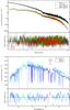 |
Fig. 5 As in Fig. 4 for HE 1143-1810. |
| In the text | |
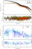 |
Fig. 6 As in Fig. 4 for CTS A08.12. |
| In the text | |
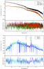 |
Fig. 7 As in Fig. 4 for Mrk 110. |
| In the text | |
Current usage metrics show cumulative count of Article Views (full-text article views including HTML views, PDF and ePub downloads, according to the available data) and Abstracts Views on Vision4Press platform.
Data correspond to usage on the plateform after 2015. The current usage metrics is available 48-96 hours after online publication and is updated daily on week days.
Initial download of the metrics may take a while.