| Issue |
A&A
Volume 530, June 2011
|
|
|---|---|---|
| Article Number | A22 | |
| Number of page(s) | 15 | |
| Section | Galactic structure, stellar clusters and populations | |
| DOI | https://doi.org/10.1051/0004-6361/201015348 | |
| Published online | 02 May 2011 | |
An empirical calibration of Lick indices using Milky Way globular clusters⋆,⋆⋆
1
Dipartimento di AstronomiaUniversita di Trieste, via G.B. Tiepolo, 11, 34127 Trieste, Italy
e-mail: This email address is being protected from spambots. You need JavaScript enabled to view it.
2
INAF - Osservatorio Astronomico di Trieste, via G.B. Tiepolo, 11, 34127 Trieste, Italy
3
Institut fur Astronomie, ETH Zurich, Wolfgang-Pauli-Str. 37, 8092 Zurich, Switzerland
Received: 6 July 2010
Accepted: 7 February 2011
Abstract
Aims. We provide an empirical calibration relation to convert Lick indices into abundances for the integrated light of old, simple stellar populations for a large range in the observed [Fe/H] and [α/Fe]. This calibration supersedes the previously adopted ones because it is based on the real abundance pattern of the stars instead of the commonly adopted metallicity scale derived from the colours.
Methods. We carried out a long-slit spectroscopic study of 23 Galactic globular clusters (GCs) for which detailed chemical abundances in stars have previously been measured. The line-strength indices, as defined by the Lick system and Serven and collaborators, were measured in low-resolution integrated spectra of the GC light. The results were compared to average abundances and abundance ratios in stars taken from the compilation by Pritzl and collaborators, as well as synthetic models.
Results. The Fe-related indices increase linearly as a function of [Fe/H] for [Fe/H] > − 2. The Mg-related indices respond in a similar way to [Mg/H] variations, although Mgb turns out to be a less reliable metallicity indicator for [Z/H] < − 1.5. Despite our knowledge of the Mg overabundance with respect to Fe in GC stars, we are unable to infer a mean [Mg/Fe] for the integrated spectra that correlates with the resolved stars properties, because the sensitivity of the indices to [Mg/Fe] is smaller at lower metallicities. We present empirical calibrations for Ca, TiO, Ba, and Eu indices, as well as the measurements of Hα and NaD.
Key words: globular clusters: general / galaxies: elliptical and lenticular, cD
Based on observations collected at the European Southern Observatory, Chile, programs 0.77B0195(A) and (B).
Appendices are available in electronic form at http://www.aanda.org
© ESO, 2011
1. Introduction
Simple stellar opulations (SSPs), namely populations of stars characterized by the same initial mass function (IMF), age, and chemical composition, are the building blocks of both real and model galaxies that consist of a mixture of several SSPs, differing in age and chemical composition according to the galactic chemical enrichment history, weighted by the star formation rate. Therefore, unraveling the information encoded in the SSPs provides direct insights into different aspects of galactic evolution. Unfortunately, for most galaxies we cannot resolve single stars. The only possible way of inferring the properties of these galaxies is to observe the integrated light coming from all the stars and attempt to infer their star formation history and chemical enrichment from either their colours or spectra. This kind of diagnostic is affected by the well-known age-metallicity degeneracy. A useful tool developed by the Lick group was a system of 25 line-strength indices (Worthey et al. 1994), which help us in disentangling the effects of age from those of metallicity. The problem is, however,complicated by a third parameter, namely the [α/Fe] abundance ratio, having a non negligible effect on the line indices.
More recently, theoretical line-strength indices tabulated for SSPs as functions of their age, metallicity and α-enhancement have been published (Thomas et al. 2003, 2010; Schiavon 2007; Lee et al. 2007).
Globular clusters (GCs) are probably the closest approximation to a SSP. Lick indices have been measured in metal-poor GCs (Burstein et al. 1984; Covino et al. 1995; Trager et al. 1998) and Galactic bulge metal-rich GCs (Puzia et al. 2002), most recently a large homogeneous sample being provided by Schiavon et al. (2005). Synthetic SSPs have usually been calibrated on the Galactic GCs (e.g. Maraston et al. 2003; Lee et al. 2009). In many cases, however, the adopted intrinsic metallicity scale was based on some generic metallicity labelled “[Fe/H]” and inferred mostly from photometric measurements (e.g. Zinn & West 1984; see also Harris 1996).
Now that high-resolution spectra of single stars in GCs are available, it is possible to test the accuracy of the SSP prediction as well as the reliability of the “inversion”(namely from measured indices to inferred abundances) technique against the true [Fe/H] (or [Mg/Fe]). It turns out that while the same SSPs that are assumed to be calibrated on the Galactic GCs perform quite well in recovering the metallicity, they fail to recover the abundance ratios. For instance, by looking at the results by Mendel et al. (2007, their Fig. 5), who tested the inversion technique for a number of widely used SSPs against the observed abundances in the stars of the GCs, one notes that the adopted stellar population models (including the most widely used by the community) neither correlate with the [Mg/Fe] observed in the stars of the GCs, nor reproduce the [Mg/Fe]-[Fe/H] relation (their Fig. 6), which is also clear for the MW GCs. The only robust inference that can be made by this method is that GCs are on average α enhanced, i.e. that α-enhanced SSPs reproduce on average the indices of Milky Way GCs more accurately than solar-scaled SSPs. We note that the vast majority of the GCs have measured indices in regions of the index-index diagrams poorly explored by the models (Mendel et al. 2007, cf. their Fig. 2), therefore the inferred abundances are often extrapolated.
Our goal is to calibrate observed Lick indices in Galactic GCs for which detailed chemical abundances in stars have been measured with high resolution spectroscopy.In particular, we use the average – over several works and several stars in each globular cluster – abundances and abundance ratios by Pritzl et al. (2005)The aim of the project is to provide an empirical calibration relation to convert Lick indices into abundances for a large range in both [Fe/H] (from –2.34 to –0.06 dex) and [α/Fe] (e.g. from –0.15 to 0.58 dex). The correlation between Lick indices such as ⟨ Fe ⟩ (or Mgb) and [Fe/H] has already been shown and discussed by other works, the latest and most accurate study being that of Puzia et al. (2002), for a very similar range in [Fe/H]. With respect to these works, our calibration is more robust in that we double the number of GCs – all of them observed by the same instrument and with the same settings – and we do not limit the analysis to GCs belonging to the Milky Way bulge (as in Puzia et al. 2002). Furthermore, we use the latest [Fe/H] ratios derived from high resolution spectroscopy, whereas previous works used a generic “metallicity”, often based on older (photometric) measurements.
Finally, a careful study of the relation between indices and the abundance of the main absorbing species at the relevant wavelengths in both our observations and in synthetic spectra, provides some possible explanation on the reason of the results by Mendel et al. (2007) discussed above.
The plan of the paper is the following. We discuss the observations and data reduction process in Sects. 2 and 3, respectively. Our results are presented in Sect. 4 and some implications are discussed in Sect. 5. Conclusions are drawn in Sect. 6.
2. Observations
We observed 23 Galactic GCs (see Table 1) during two observing runs1 at the ESO New Technology Telescope in La Silla using EMMI (Dekker et al. 1986). We used the low-resolution RILD Grism 5, which covers a wavelength range ~380−700 nm with a dispersion of 55 nm/mm, 1 × 1 binning, and slow read-out to reduce the noise. One pixel corresponds to 0.166′′. The slit width was set to 2′′. The resulting resolution is ~10 Å FWHM, very close to the actual nominal ~8.4−10 Å resolution that the Lick system has in the wavelength range relevant for our study. This set-up was chosen to minimise the correction otherwise needed to set the observed spectra into the Lick resolution.
Spectra were taken with the slit in two different angles (east-west and north-south direction) for each cluster, to avoid abnormal contribution from individual bright stars and to select a sample of the typical underlying stellar population.
Individual exposures were adjusted to avoid saturation. We separate our sample into two runs to ensure the observability of each object at low air-masses. We estimated the exposures time by means of the ETC – Optical Spectroscopy Mode Version 3.0.6 – tool. In particular, we used the central surface brightness in the V band provided by the 2003 update of the Harris (1996) catalogue for our sample of GCs and required a signal-to-noise ration (S/N) of 50, for an airmass ≤ 1.3, and seeing below 2′′. To give an example, we found an exposure time of ~100 s for bright objects (i.e. V surface brightness ~14−15 mag/arcsec2) and ~6800 s for the faintest ones (i.e. V surface brightness >19 mag/arcsec2). However, to reduce cosmic-ray events, several shorter exposures of each target were taken and then added together. Lick standard stars were observed each night. The stars were slightly defocused to avoid saturation.
We observed under cloudy conditions during the first half of the first night and for most of the last night. The science frames acquired during these period were not used in the following discussion. Moreover, during the last night we had to discard some GCs in the original proposal list, because they were no longer visible when the weather conditions improved.
List of targets.
3. Data reduction
We performed the standard data reduction steps using the ESO MIDAS software. In particular, dark current and bias were removed and the images were flat-fielded by means of calibration frames acquired every night. Science frames were cleaned of cosmic rays and bad pixels, then calibrated in wavelength by means of a He-Ar lamp frame and finally rebinned. Wavelength calibration was checked on the sky lines of science frames. Sky lines were also used to estimate the (negligible) variable vignetting along the slit. The sky spectrum was estimated from regions at the edges of the science frames. The variability of the sky lines and stellar crowding hampered us from using separate sky frames that we took during the observing runs in a homogeneous way for all clusters. A comparison between the two methods is presented in the Appendix (Table A.1). The actual resolution of the observations (~10 Å) was confirmed from the width of both sky lines and calibration frames. Finally, after correcting for the atmospheric extinction, one-dimensional integrated spectra were created by carefully avoiding bright stars and taking only the central ~1.5 arcmin (along the slit) of the entire frame, to maximize the S/N ratio. The typical value of the S/N per pixel at the central wavelength is ~50. At each step of the reduction process, we also propagated the statistical error starting from the Poisson noise of the science frame, the read-out-noise of EMMI and the sky subtraction as in Carollo et al. (1993, their Eq. (1)). We thus created an error spectrum.
Line-strength indices were measured by using of a suitable routine ( ) in the
  package (Graves & Schiavon 2008). The code measures all Lick indices – according to the Trager et al. (1998) definition.We modified the routine to also measure indices as defined by Serven et al. (2005) and the Hα index defined in Cohen et al. (1998). The error spectra are used to calculate the error associated with each measured index as in Cardiel et al. (1998, cf. their Eq. (20)). We repeated this procedure for the two slit positions for each GC. The reader interested in these intermediate steps is referred to the Appendix, where we show examples of the most widely used indices in Table B.1 along with their statistical errors. As expected (e.g. Cardiel et al. 1998), the high S/N of our spectra implies statistical uncertainties of the order of a few percent in the majority of the cases. For each cluster, we show the measurements in both EW and NS directions along with their statistical uncertainties. Whilst for the majority of the observed objects the values for a given index taken along the two directions of the same cluster are very close, they might disagree at more than the 3σ level if only statistical errors were taken into account. These variations reflect the different sampling of the stellar light at different positions in the same cluster and give an idea of the intrinsic spread within one cluster. We took the average of the two measurements as the representative value of that index for a given cluster. We use the difference between the two directions as the estimate of the uncertainty associated with a given index. In particular, we use half of the difference as an estimate of the error. These values are shown in Table B.2. We applied small corrections if the spectra were at a resolution (as in our case) lower than the Lick/IDS system. Since our resolution is about the same as the Lick system, these corrections are minimal (cf. examples in Table C.2).
Final corrected Lick indices – I.
Final corrected Lick indices – II.
Hα and Serven et al.’s indices.
As far as the Lick indices are concerned, the final step requires us to set our measurements on the Lick system. In practice, reduction steps, such as the wavelength calibration and the smoothing of the spectra, always leave some residual offset from the standard reference frame set by the Lick group (see Worthey et al. 1992). The typical way to tackle the issue is to observe and reduce Lick standard stars (Worthey et al. 1994)2 and compare the measured indices with those published by the Lick group (e.g. Worthey et al. 1992). If some systematic offset is present, it is common to correct the observed indices in order to place them on the Lick system. For the more relevant indices, we found that the measured Hβ values for the Lick standard stars that we observed are consistent, within the errors, with the values given by the Lick group. Therefore, no correction has been applied. The same was true for the indices Fe5015,Ca4227, TiO1 , TiO2, and NaD. In contrast, small corrections were instead applied to the indicesMg2 (0.024 mag), Mgb (0.12 Å), and Fe5270 (0.17 Å). We found that a correction that depends on the index strength was necessary for the index Fe5335, and therefore discarded it from the discussion. A comparison with the literature (e.g. Puzia et al. 2002) demonstrates that our adopted corrections are very similar to those in previous works. While Cohen et al. (1998) measured their indices at a resolution of ~8 Å, the Serven et al. (2005) indices were introduced and tested in relation to a massive elliptical galaxy with 200 km s-1 velocity dispersion. We chose to present the measurements for these indices at our native resolution, without any further correction.The sample of final corrected most widely used Lick indices is presented in Tables 2 and 3, whereas Table 4 shows some non-Lick indices. Other Lick and Serven et al.’s indices are available upon request. We do not associate an error with the above-mentioned procedure, and the final error we provided is the difference between the two directions. We then compared our measurements with available indices from Puzia et al. (2002 and references therein), Trager et al. (1998) and Graves & Schiavon (2008), the typical differences between our results and the literature being ~10%. When the same GC had been observed by more than one author, that the differences between authors and between one author and ourselves were found to be comparable to the differences between our measurements along the EW and NS directions.
4. Results
We present the main results of this project, namely an empirical calibration between observed indices and abundances (and abundance ratios) measured in the stars. After a brief review of the index-index properties of our GC sample, we introduce the most widely used metallicity indicator, i.e. [Fe/H]. We then study the Mg, Ca, Ti, Eu, and Ba abundances.
4.1. Index-index diagrams
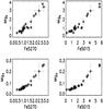 |
Fig. 1 Relation between observed Mg- and Fe-related indices. |
In Fig. 1, we present the relation between observed Mg- and Fe-related indices measured in this work.
The reader should note that our finding that the Mgb-Fe5270 relation tends to deviate more and more from the 1:1 relation as Fe5250 (and hence the metallicity) increases, does not mean that the α-enhancement increases as well, as we see in the remainder of the paper. As expected from chemical evolution studies of the Milky Way (e.g., Matteucci 2001), we know that [α/Fe] decreases with [Fe/H], after a plateau, at [Fe/H] ~ −1. This trend is also evident in the entire sample of GCs by Pritzl et al. (2005).
In Fig. 2, we show that higher values for the Hβ index correspond to lower values of metallicity-related indices. This is not unexpected (see also Puzia et al. 2002; Burstein et al. 1984): the more metal poor, the bluer the horizontal branch (e.g. Schiavon et al. 2004; Lee et al. 2009). Here we do not revisit the issue and only conclude that this hampers the use of the Hβ index as a pure age indicator, owing to its dependence on the horizontal branch morphology. For the sake of the following discussion, we note that models (e.g. Lee et al. 2009) show that the horizontal branch has little (if any) effect on the metal indices that we study. In addition, Hβ exhibits an almost 1:1 correlation with Hα (squares in Fig. 3). This relation is tighter and somewhat steeper than the one found by using the M 87 GCs by Cohen et al. (1998) (asterisks in Fig. 3). However, the distribution in the values of the Hα index in M 87 and our sub-sample of Milky Way globular clusters are remarkably similar (Fig. 4). We refrain from a more in-depth interpretation given the large difference in size between the two samples. We note that the Hα index has been shown by Serven et al. (2010) to provide a useful independent estimate to correct the Hβ index for emission in galaxies. Similarly, Poole et al. (2010) estimate the contamination from active M dwarfs to their Milky Way GC spectra.
[X/H] = a × Index + b relations.
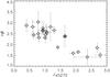 |
Fig. 2 Relation between observed Hβ and Fe5270 indices. |
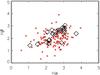 |
Fig. 3 Relation between observed Hβ and Hα indices. Diamonds: Milky Way GCs (this work); asterisks: M 87 GCs from Cohen et al. (1998). |
4.2. An empirical calibration for the GC [Fe/H]
In Fig. 5, we present the Fe-related index Fe5015 and Fe5270 versus themean Fe abundance in the stars of the GCs given by Pritzl et al. (2005). The solid lines in Fig. 5 are obtained by performing a formal linear regression to the points and the coefficients of the relations [Fe/H] = a × Index + b are given in Table 5 along with the correlation coefficients r. In calculating these relations, we implicitly kept the age fixed. Therefore we warn the reader not to blindly use these calibrations in external galaxies, where they can lead to an underestimate of the metallicity if a younger (sub-)population of GCs exists. As expected, very tight linear relations relate the Fe-indices to the [Fe/H] abundance. We note that, even if several GCs display evidence of multiple stellar populations, the Fe content of their stars is highly homogeneous to within ~10% (Carretta et al. 2009). A very similar calibration can be obtained if one uses the metallicity scale by Zinn & West (1984) as in the Harris (1996) catalogue. In particular, we find that [Fe/H] = 0.76 Fe5270 − 2.22. A new metallicity scale based on high resolution spectra has been released by Carretta et al. (2009). We have nine GCs in common with Carretta et al.’s sample. Their new [Fe/H] abundances are within a few percent of the values from Pritzl et al. that we adopted in this paper, so we do not expect significant variations in the calibration even if this more recent and homogeneous metallicity scale were adopted.
Our results are also in agreement with Puzia et al. (2002)’s findings. However, two significant improvements are present: i) we do not limit the analysis to Milky Way bulge GCs; ii) the empirical calibration relation between indices and abundances is based on abundances measured in stars using high resolution spectra, whereas previous works were based on some metallicity scale derived mostly from photometric colours.
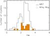 |
Fig. 4 Distribution for the values of the Hα index in M 87 (solid, Cohen et al. 1998) and the Milky Way (this work, dashed and shaded histogram). |
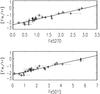 |
Fig. 5 Average [Fe/H] in stars by Pritzl et al. versus Fe-related Lick indices (this work). The solid line is the formal linear regression. |
Such a remarkable linear behaviour between the index and the logarithm of the main absorber can be analysed by performing of curve of growth analysis. A qualitative explanation of the relation can indeed be attempted using synthetic spectra of a K0 giant (Bonifacio, priv. comm.). We show below that more detailed models of a SSP yield consistent results. Indices such as Fe5270 are measured in Å of equivalent width (EW), hence a curve-of-growth-like diagram can be easily made by plotting, e.g. log (Fe5270) vs. [Fe/H]. Fig. 6 shows the curve-of-growth-like diagram for our synthetic spectra, the solid line being a formal linear fit and the dashed one giving the 1:1 relation. Overall, we find that log (Fe5270) ~ 0.4 × [Fe/H] , i.e. it appears to diverge away from the linear regime (where log EW ~ 1 × log abundance, dashed line) at [Fe/H] ~ −2 and it enters the logarithmic saturated one (where EW ~ log abundance, hence index ~ [Fe/H] ). This conclusion is corroborated by inspection of the lines in the high resolution synthetic spectrum and also holds for the Fe5015 index. In addition, the reader should note that, according to Tripicco & Bell (1995), this index seems to be sensitive to Mg, Ti, and the total metallicity Z rather than Fe. An important caveat applies to the discussion: strictly speaking the curve of growth as a function of abundance applies to a single absorption line, whereas the EW of each Lick index typically includes contributions from several lines, not all related to the most important absorbing species at those wavelengths. In practice, Fe and Mg indices are sensitive to variations in, e.g., Ca, C, and Ti abundances (e.g. Thomas et al. 2003; Lee et al. 2009).Moreover, because the true spectroscopic continuum is altered by the low resolution, and because the index definition pseudocontinua bands cannot account for this change, there will always be some shift and change of slope in index values compared to a true curve-of-growth analysis.
We note that these different regimes of the curve of growth were not taken into account in the calculation of α-enhanced indices as in Thomas et al. (2003). The linear regime, instead, was a common assumption. An assessment of the error is beyond the scope of the paper, and likely unnecessary because in more recent models (e.g. Lee et al. 2009) the variation in the index is derived by analysing an extensive library of synthetic spectra and isochrones for several chemical compositions. The use of a Mg-enhanced composition for generating the spectra do not alter these conclusions.
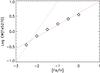 |
Fig. 6 Curve of growth-like diagram for the Fe5270 absorption as modelled by the solar-scaled spectra of a K0 giant star. The solid line is the formal linear regression. The dashed line gives the 1:1 relation as if the linear regime held up to [Fe/H] ≃ − 2. |
4.3. An empirical calibration for the GC [Mg/H]
A similar analysis with the Mg-related indices (Fig. 7) shows that [Mg/H] scales with Mg2 and Mgb. In addition, they both roughly scale with metallicity. However, at low values of the indices, the relations deviate from a straight line.
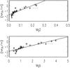 |
Fig. 7 Average [Mg/H] in stars by Pritzl et al. versus Mg-related Lick indices (this work). The solid line is the formal linear regression. |
We now try to explainthis loss of sensitivity to changes in the Mg abundance: in the inset of Fig. 8, we show the Mg2 index predicted by our K0 giant spectrum as a function of the [Mg/H] abundance in the star. A quadratic relation between Mg-indices and [Mg/H] (see also Puzia et al. 2002) provides a more accurate fit than the simple linear relation and is expected from the index-index diagrams presented in Sect. 4.1. We can again understand this behavior in terms of curve of growth. We first notice that the Mg2 index is the only one in the subset of Lick indices studied here that is defined in magnitudes. Moreover, it is not defined as the EW of the absorption features in the Mg2 bandpass. Therefore, some algebra is required to derive the EW from the measure of the Mg2. The behavior of the EW(Mg2) as a function of [Mg/H] (main panel of Fig. 8) arrives again in the flat region of the curve of growth and explains the relation between Mg2 and [Mg/H] as a result of the non-linear relation between Mg2 and EW(Mg2). The main conclusion, however, is that below [Mg/H] = −1.5, the Mg2 index is not a good measure of either the Mg abundance or the total metallicity.
A similar behavior (and conclusion) applies to the Mgb index. In this case, however, an inspection of the high resolution spectra tells us that it is the competition between the Mgb lines and other metal lines (mostly from Ca, Ti, and Fe) in the flanking bands that makes the index insensitive to abundance changes at [Mg/H] below −1.5. This is because, while the former lines have cores that saturate at quite low [Mg/H], the latter saturate at slightly higher values for [Mg/H]. In practice, changes in the depth of the central absorption features seem to be compensated by the changes in the pseudo-continuum. The results are unchanged if one uses synthetic spectra of a star with an Mg-enhanced composition. These predictions show a remarkable qualitative agreement with those derived for integrated spectra of a SSP by Lee et al. (2008). We therefore argue that our discussion based on the scrutiny of a single star can be extended to the general case of a SSP, at least as a partial explanation. Other studies (Maraston et al. 2003) showed that at low metallicities the Mg indices of a SSP tend to be dominated by the lower main sequence, making them prone to being affected by changes in the IMF due to the dynamical evolution of the GCs. This is probably why the indices calculated in a single K0 giant star are weaker than both those measured in our GC sample and those predicted by a theoretical SSP with a Salpeter (1955) IMF.
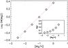 |
Fig. 8 Curve-of-growth-like diagram for the EW(Mg2) as modelled by the solar-scaled spectra of a K0 giant star. The solid line is the formal linear regression. The inset shows the Mg2 index as a function of the Mg abundance. |
4.4. An empirical calibration for other α elements
Apart from the well-studied Mg and Fe indices, the high resolution data enable us to provide – for the first time – empirical calibrations for other elements. We start with the results of two Ca-indices, namely Ca4227 and Ca4455 (on the Lick system). They track each other very well (Fig. 10) and correlate with the average Ca abundance measured in stars given by Pritzl et al. (2005), as shown in Fig. 11. The empirical calibrations are given in Table 5.
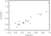 |
Fig. 9 Average [Ca/H] in stars by Pritzl et al. versus a Ca-related Lick index. |
Ti is another element commonly enhanced in a similar way to other α elements. Here we note that the TiO1 index trend with [Ti/H] is not linear, since the index is measured in magnitudes (as we have seen for the Mg2). Therefore we do not provide a linear fit to the empirical calibration. We have found that the index TiO2 closely tracks TiO1, therefore we have a similar trend with [Ti/H] (not shown here). As we briefly discuss below for Mg, none of these other enhanced elements offers a simple way to infer a calibration for the [α/Fe] ratio.
4.5. An empirical calibration for neutron rich elements
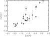 |
Fig. 10 Ca index-index diagram. |
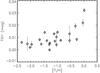 |
Fig. 11 Average [Ti/H] in stars by Pritzl et al. versus a Ti-related Lick index. |
Serven et al. (2005) also defined indices that allow the study of neutron-rich elements. In this section, we adopt two of them to study the abundance of a typical r-process element (Eu) and a typical s-process element (Ba). In Fig. 12, we show the results for the Eu index, Eu4592, from Serven et al. (2005). The results for Ba4552 are shown in Fig. 13. The empirical calibrations are given in Table 5. We note that the relations involving Ba and Eu are less tight than the those for Fe and Mg. This is because the Serven et al. indices are designed for very high ( > 100) S/N data, whereas our data typically have a S/N of at most 40 at the relevant wavelengths. Nonetheless, finding this correlation is important because, to our knowledge, this is the first time that these indices have been tested for such a large metallicity range. However, we stress that further work will be required to demonstrate that at our resolution and S/N the contribution from other metals (mainly Fe) is negligible and that the correlations shown in the figures are really due to an abundance increase.
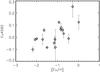 |
Fig. 12 Average [Eu/H] in stars by Pritzl et al. versus a Eu-related index from Serven et al. (2005). |
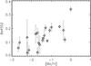 |
Fig. 13 Average [Ba/H] in stars by Pritzl et al. versus a Ba-related index from Serven et al. (2005). |
5. Discussion
One possible additional step in our analysis could have been to transform the indices into [Fe/H] abundances by means of the standard inversion technique3. Although we decided to use the package, we could not because the metallicity grid (based on Schiavon 2007, tracks) on which is based does not allow inversion at [Fe/H] below − 1.3 and − 0.8 for the solar-scaled and the α-enhanced cases, respectively, whereas, according to Pritzl et al. most of our GCs are below these limits.
As for other SSPs, such as those by Thomas et al. (2003, and subsequent improvements), we refer to Mendel et al. (2009) and Lee et al. (2009) who did a thorough testing on GC data and found a reasonable agreement between the SSP-inferred [Fe/H] and metallicity estimates based on resolved stellar populations (the former author) and GC metallicity scales (the latter). We note that almost all the tracks tested by Mendel et al. (2007) to transform the line-strength indices into abundance ratios fail to provide an accurate α-enhancements as a function of Fe abundance, namely they cannot reproduce the observed [Mg/Fe]-[Fe/H] relation observed in the stars of the same GCs (Pritzl et al. 2005 – see Fig. 6 in Mendel et al. 2007). Whether this is an intrinsic problem of the SSP libraries or is rooted in the inversion technique remains to be understood. This problem is somewhat expected from the above analysis. We found that [Fe/H] < − 1 is extremely difficult to discriminate between a track pertaining to the solar composition and one built assuming a +0.4 dex enhancement in the [Mg/Fe] ratio.
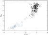 |
Fig. 14 Position in the index-index diagram of our GCs (triangles) and a sample of elliptical galaxies (asterisks, Thomas et al. 2005). |
Our findings provide a tentative explanation of the difficulties encountered by other works. For instance, Puzia et al. (2005) found it difficult to discriminate between α-enhanced and solar-scaled (extra-galactic) GCs at below Mg2 ~ 0.2 mag and ⟨ Fe ⟩ below 2 Å. By using the relations derived in the previous sections (e.g. Fig. 5), these values correspond to [Fe/H] < −1, i.e. to where the theoretical curves in the index-index plane come closer and closer.Similarly, this happens in the recent update of the Thomas et al. (2003) stellar population models (Thomas et al. 2011).
If theoretical models with different α-enhancement differ so little, clearly errors in the measurements may render impossible the derivation of the true [Mg/Fe] ratio in the [Fe/H] < −1 regime. This has interesting consequences, since high resolution spectra from GC stars show a typical level of α-enhancement (0.3 dex) comparable (and in a few cases even higher) to values typical of massive ellipticals.
For elliptical galaxies, although the relation between Mg-related indices and Fe-related ones is a continuation of the overall trend seen in GCs (Fig. 14), it is sistematically steeper (Burstein et al. 1984; Worthey et al. 1992). The original interpretation (Burstein et al. 1984) was that something else (i.e. [Mg/Fe] enhancement) contributes to the galaxy Mgb excess. Whilst GCs can be considered SSPs, elliptical galaxies cannot. They are a composite stellar population made of several SSPs. This implies that the location in the Mgb-Fe5270 diagram (or an equivalent measure) indicates the average value over several SSPs that formed during the galactic evolution.
We expect the first SSPs forming in these galaxies to contribute more to the total light because of the higher blue/optical luminosity with respect to later SSPs4. In other words, a composite stellar population must have a higher average metallicity than a SSP featuring the same line-strength index (Greggio 1997), because the lowest metallicity tail of the stellar metallicity distribution has a non-negligible role in the integrated spectrum. In the light of our results for GCs, we expect the first SSPs to have little impact on the Mg-related index. Even if they are the most α-enhanced SSPs in the galaxy, since they formed only out of SNII ejecta, their Mg-related indices will be fairly low and indistinguishable from those of a solar-scaled SSP. Therefore, one may be tempted to say that the α-enhancement that we “measure” in galaxies is lower than the true α-enhancement. With the help of Fig. 15, we show that this is (luckily) not the case. The solid line is the stellar mass distribution as a function of [Mg/Fe] predicted by the Pipino & Matteucci (2004, PM04) chemical evolution model for a typical massive elliptical galaxy. The mass-weighted average of this distribution is ⟨ [Mg/Fe] true, ∗ ⟩ = 0.43 dex. This is the true average that an observer would wish to obtain by inverting indices into abundances. In reality, the observed quantity is a luminosity-weighted value. We convert the stellar mass distribution into the stellar luminosity distribution as a function of [Mg/Fe] (dotted line) by using the M/L ratio for a 12 Gyr old SSP with Salpeter IMF as a function of [Fe/H] from Maraston et al. (2003). The predicted luminosity average is ⟨ [Mg/Fe] true, lum ⟩ = 0.45 dex. We now assume that not all the SSPs that make our galaxy contribute to the measurement of the α-enhancement. In particular, the dashed line gives the luminosity distribution when the SSPs formed with [Fe/H] < −1 are not taken into account. We previously chose [Fe/H] = −1 as the limiting boundary because we showed that below such a limit the [Mg/Fe] does not make any difference to the predicted Mg- related indices. The average [Mg/Fe] inferred from this last distribution is ⟨ [Mg/Fe] obs ⟩ = 0.38 dex. This exercise shows that the [Mg/Fe] will only be underestimated by a modest amount (0.05 dex). A lower mass elliptical, with a more extended and quieter star formation history than the example displayed in Fig. 15 might have a larger proportion of SSPs formed with [Fe/H] < −1, hence a more significant underestimate of its ⟨ [Mg/Fe] true ⟩ . A further analysis would require a proper weighting of the fluxes of all the stars involved according to their spectral type, which is beyond the scope of the present paper.
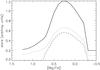 |
Fig. 15 Stellar mass distribution as a function of [Mg/Fe] predicted by the PM04 chemical evolution model for a typical elliptical galaxy (solid line). The luminosity distribution as a function of [Mg/Fe] is given by the dotted line. The dashed line gives the luminosity distribution when the SSPs formed at [Fe/H] < −1 are not taken into account (see text). The curves have been arbitrarily rescaled to the same value and offset to make differences in the tails more visible. |
Finally, we note that Mg displays a large star-to-star variation in anti-correlation with Al (e.g. Carretta et al. 2010 and references therein, Gratton et al. 2004) because of self-enrichment by AGB stars (e.g. D’Antona & Ventura 2007) or rotating stars (Decressin et al. 2007) and possibly related to the presence of at least two stellar generations in most GCs (Carretta et al. 2009; D’ercole et al. 2009). Unfortunately, Al indices are not included in the Lick ones,and our S/N is not high enough to have an accurate measurement of the Al3953 index defined by Serven et al. (2005), therefore we have no means of acquiring a deeper insight with the low-resolution integrated light spectroscopy. A promising tool may be high-resolution integrated light spectroscopy (e.g. McWilliam & Bernestein 2008).
6. Conclusions
We have carried out a long-slit spectroscopic study of 23 Galactic GCs for which detailed chemical abundances in stars have been measured. We measured metallicity indices defined by the Lick system, Cohen et al. (1998), and Serven et al. (2005) in low-resolution integrated spectra of the GC light. We compared them to average abundances and abundance ratios in their stars taken from the compilation by Pritzl et al. (2005) as well as to synthetic models.
We provided an empirical calibration relation to convert these indices into abundances for a large range in the observed [Fe/H] and [alpha/Fe]. The Mg- and Fe-metallicity calibrations supersede the previously adopted ones because they are based on the real abundance pattern of the stars instead of the commonly adopted metallicity scale derived from, e.g., colours. We presented novel calibrations for Ca, Ti, Ba, and Eu based on the same set of average abundances in stars.
Below we summarize our main results:
-
For the first time we present the Hα index (Cohen et al. 1998) for Milky Way GCs. In our GCs, Hβ tracks Hα very well. The distribution of the values of Hα is similar to that inferred by Cohen et al. (1998) for M 87.
-
Calibration of [Fe/H] as a function of Fe-indices is the most robust estimator of the GC metallicity (also because the small star-to-star variation in [Fe/H]). The relation between indices and [Fe/H] is linear to a good approximation at [Fe/H] > −2, when a regime similar to the saturated regime of the curve of growth sets in.
-
Mg-indices are not reliable below [Mg/H] = −1.5 for effects due to the contribution of metal lines to the pseudocontinuum and, possibly, IMF effects.
-
At [Fe/H], [Mg/H] < − 1.5, it is impossible to measure the effect of [Mg/Fe] in the spectra. At (slightly) higher metallicities, poor statistics, errors, and star-to-star variations within GCs hampered us from deriving a simple relation between [Mg/Fe] and (a combination of) indices. Only in the very high metallicity regime of elliptical galaxies is it possible to safely use Mg- and Fe-indices to infer the mean [Mg/Fe] in stars.
-
Since a small fraction of low-metallicity α-enhanced stars do exist in elliptical galaxies, we estimate that the SSP-equivalent value of the [Mg/Fe] might underestimate the true average value of their stellar populations.
-
We showed that the Lick Ca- and TiO-indices correlate with [Ca/H] and [Ti/H], respectively. The relations are less tight than those of Mg case. In addition, these α elements do not allow the construction of a reliable calibration for measuring the global α-enhancement.
-
We illustrated that the Serven et al. (2005) Eu and Ba indices correlate with [Eu/H] and [Ba/H], respectively, although with a larger scatter than in the Mg- and Fe-metallicity calibration.
Online material
Appendix A: Sky subtraction
In this Appendix, we provide two examples of the results for different methods of sky subtraction for a subset of the measured indices. As discussed in the main text, night sky variability and the location of some GCs in crowded fields did not allow us to always find a suitable region close enough to the target that could be used as an external sky frame. When it was possible however, the difference in the results with respect to the sky estimate from the edges of the science frame was very small, especially in the case of metal lines. We note here that for the same two clusters, Puzia et al. (2002) found a larger difference between the two ways of accounting for the sky background. This maybe the consequence of the target region chosen to measure the sky spectrum. However, based on our tests, we agree with the results of these authors that the internal derivation of the background is more reliable.
Uncorrected Lick indices. Example of same-frame sky estimate versus external frame.
Appendix B: Uncorrected indices
We show the uncorrected Lick indices (after sky subtraction) measured along the two directions for each individual cluster (Table B.1) as well as their average (Table B.2). We refer to the main body of the paper for details. We recall that, by “uncorrected” we mean data that have not (yet) been corrected for any offset between our and the Lick system caused by, e.g., residuals in the sky subtraction, and systematics in the wavelength calibration. The example is limited to a subset of the measured indices, the remainder of the sample being available upon request.
Lick indices measured along EW and NS directions and their associated statistical uncertainties.
Uncorrected Lick indices averaged over the two directions.
Appendix C: Effect of the correction to the Lick resolution
We present the uncorrected indices averaged over the two directions measured as if our observational set-up were in the native Lick resolution. The entries in Table C.1 should be compared to those in Table B.2. Here we also measure the indices assuming that our resolution precisely matches that of the Lick system (e.g. Worthey & Ottaviani 1997). Our resolution is slightly lower, hence a small correction is in principle needed (see Sect. 3), which however we do not apply here. The difference (Table C.2) in the end-products is remarkably small, typically being < 1% for Hβ and Mg2, and 3–4% for the other indices shown in the table.
Uncorrected indices averaged over the two directions – Indices measured as if they were at the native Lick resolution.
Applied velocity dispersion corrections.
Run A:3 nights is May 2006 – run B:one night in September 2006.
Available at: http://astro.wsu.edu/worthey/html/system.html
A minimization technique that yields the best-fit abundances and age for a given set of measured indices and a specific SSP model.
Line blanketing in metal richer populations suppress the flux in the wavelengths where the spectra are taken. We also note that the average ages and the average α enhancement imply that the SSPs are rather old (above 10 Gyr) and that the spread in ages in a single galaxy should not exceed ~1 Gyr. Therefore we neglect age effects in this discussion.
Acknowledgments
We warmly thank the referee, G. Worthey, for suggestions that improved the quality of the paper, E. Pompei for her invaluable help during the observing runs, S. Samurovic for providing help with MIDAS at the beginning of this work and P. Bonifacio for providing synthetic spectra. We acknowledge useful discussions from G. Graves, M. Koleva, H.-C. Lee, M. Sarzi, A. McWilliam, and P. Sanchez-Blazquez. This research has made use of: the SIMBAD database, operated at CDS, Strasbourg, France; the Harris Catalog of Parameters for Milky Way Globular Clusters – Feb. 2003 revision – available at http://physwww.mcmaster.ca/ the Lick/IDS data mantained by G. Worthey (http://astro.wsu.edu/worthey/html/system.html).
References
- Burstein, D., Faber, S. M., Gaskell, C. M., & Krumm, N. 1984, ApJ, 287, 586 [NASA ADS] [CrossRef] [Google Scholar]
- Cardiel, N., Gorgas, J., Cenarro, J., & Gonzalez, J. J. 1998, A&AS, 127, 597 [NASA ADS] [CrossRef] [EDP Sciences] [Google Scholar]
- Carollo, C. M., Danziger, I. J., & Buson, L. 1993, MNRAS, 265, 553 [NASA ADS] [CrossRef] [Google Scholar]
- Carretta, E., Bragaglia, A., Gratton, R., D’Orazi, V., & Lucatello, S. 2009, A&A, 508, 695 [NASA ADS] [CrossRef] [EDP Sciences] [Google Scholar]
- Carretta, E., Bragaglia, A., Gratton, R., et al. 2010, A&A, 516, A55 [NASA ADS] [CrossRef] [EDP Sciences] [Google Scholar]
- Cohen, J. G., Blakeslee, J. P., & Ryzhov, A. 1998, ApJ, 496, 808 [NASA ADS] [CrossRef] [Google Scholar]
- Covino, S., Galletti, S., & Pasinetti, L. E. 1995, A&A, 303, 79 [NASA ADS] [Google Scholar]
- Decressin, T., Charbonnel, C., Siess, L., et al. 2009, A&A, 505, 727 [NASA ADS] [CrossRef] [EDP Sciences] [Google Scholar]
- Dekker, H., Delabre, B., & D’Odorico, S. 1986, SPIE, 627, 39 [Google Scholar]
- D’Ercole, A., Vesperini, E., D’Antona, F., McMillan, S. L. W., & Recchi, S. 2008, MNRAS, 391, 825 [NASA ADS] [CrossRef] [Google Scholar]
- Gratton, R., Sneden, C., & Carretta, E. 2004, ARA&A, 42, 385 [NASA ADS] [CrossRef] [Google Scholar]
- Graves, G. J., & Schiavon, R. P. 2008, ApJS, 177, 446 [NASA ADS] [CrossRef] [Google Scholar]
- Greggio, L. 1997, MNRAS, 285, 151 [NASA ADS] [Google Scholar]
- Harris, W. E. 1996, AJ, 112, 1487 [NASA ADS] [CrossRef] [Google Scholar]
- Lee, H.-C., & Worthey, G. 2005, ApJS, 160, 176 [NASA ADS] [CrossRef] [Google Scholar]
- Lee, H.-C., Worthey, G., & Dotter, A. 2009a, AJ, 138, 1442 [NASA ADS] [CrossRef] [Google Scholar]
- Lee, H.-C., Worthey, G., Dotter, A., et al. 2009b, ApJ, 694, 902 [NASA ADS] [CrossRef] [Google Scholar]
- Lee, J.-W., Kang, Y.-W., Lee, J., & Lee, Y.-W. 2009c, Nature, 462, 480 [NASA ADS] [CrossRef] [PubMed] [Google Scholar]
- Maraston, C., Greggio, L., Renzini, A., et al. 2003, A&A, 400, 823 [NASA ADS] [CrossRef] [EDP Sciences] [Google Scholar]
- Matteucci, F. 1994, A&A, 288, 57 [NASA ADS] [Google Scholar]
- Matteucci, F. 2001, ASSL, 253 [Google Scholar]
- McWilliam, A., & Bernstein, R. A. 2008, ApJ, 684, 326 [NASA ADS] [CrossRef] [Google Scholar]
- Mendel, J. T., Proctor, R. N., & Forbes, D. A. 2007, MNRAS, 379, 1618 [NASA ADS] [CrossRef] [Google Scholar]
- Pipino, A., & Matteucci, F. 2004, MNRAS, 347, 968 [NASA ADS] [CrossRef] [Google Scholar]
- Poole, V., Worthey, G., Lee, H.-C., & Serven, J. 2010, AJ, 139, 809 [NASA ADS] [CrossRef] [Google Scholar]
- Pritzl, B. J., Venn, K. A., & Irwin, M. 2005, AJ, 130, 2140 [NASA ADS] [CrossRef] [Google Scholar]
- Puzia, T. H., Saglia, R. P., Kissler-Patig, M., et al. 2002, A&A, 395, 45 [NASA ADS] [CrossRef] [EDP Sciences] [Google Scholar]
- Renzini, A. 2007, ASPC, 380, 309 [NASA ADS] [Google Scholar]
- Salpeter, E. E. 1955, ApJ, 121, 161 [Google Scholar]
- Schiavon, R. P. 2007, ApJS, 171, 146 [NASA ADS] [CrossRef] [Google Scholar]
- Schiavon, R. P., Rose, J. A., Courteau, S., & MacArthur, L. A. 2004, ApJ, 608, L33 [NASA ADS] [CrossRef] [Google Scholar]
- Schiavon, R. P., Rose, J. A., Courteau, S., & MacArthur, L. A. 2005, ApJS, 160, 163 [NASA ADS] [CrossRef] [Google Scholar]
- Serven, J., & Worthey, G. 2010, AJ, 140, 152 [NASA ADS] [CrossRef] [Google Scholar]
- Serven, J., Worthey, G., & Briley, M. M. 2005, ApJ, 627, 754 [NASA ADS] [CrossRef] [Google Scholar]
- Thomas, D., Maraston, C., & Bender, R. 2003, MNRAS, 339, 897 [NASA ADS] [CrossRef] [Google Scholar]
- Thomas, D., Maraston, C., Bender, R., & Mendes de Oliveira C. 2005, ApJ, 621, 673 [NASA ADS] [CrossRef] [Google Scholar]
- Thomas, D., Johansson, J., & Maraston, C. 2011, MNRAS, accepted [Google Scholar]
- Trager, S. C., Worthey, G., Faber, S. M., Burstein, D., & Gonzalez, J. J. 1998, ApJS, 116, 1 [NASA ADS] [CrossRef] [MathSciNet] [Google Scholar]
- Tripicco, M. J., & Bell, R. A. 1995, AJ, 110, 3035 [Google Scholar]
- Ventura, P., & D’Antona, F. 2009, A&A, 499, 835 [NASA ADS] [CrossRef] [EDP Sciences] [Google Scholar]
- Worthey, G., & Ottaviani, D. L. 1997, ApJS, 111, 377 [NASA ADS] [CrossRef] [Google Scholar]
- Worthey, G., Faber, S. M., & Gonzalez, J. J. 1992, ApJ, 398, 69 [NASA ADS] [CrossRef] [Google Scholar]
- Worthey, G., Faber, S. M., Gonzalez, J. J., & Burstein, D. 1994, ApJS, 94, 687 [NASA ADS] [CrossRef] [Google Scholar]
- Zinn, R., & West, M. J. 1984, ApJS, 55, 45 [NASA ADS] [CrossRef] [Google Scholar]
All Tables
Uncorrected Lick indices. Example of same-frame sky estimate versus external frame.
Lick indices measured along EW and NS directions and their associated statistical uncertainties.
Uncorrected indices averaged over the two directions – Indices measured as if they were at the native Lick resolution.
All Figures
|
Fig. 1 Relation between observed Mg- and Fe-related indices. |
| In the text | |
|
Fig. 2 Relation between observed Hβ and Fe5270 indices. |
| In the text | |
|
Fig. 3 Relation between observed Hβ and Hα indices. Diamonds: Milky Way GCs (this work); asterisks: M 87 GCs from Cohen et al. (1998). |
| In the text | |
|
Fig. 4 Distribution for the values of the Hα index in M 87 (solid, Cohen et al. 1998) and the Milky Way (this work, dashed and shaded histogram). |
| In the text | |
|
Fig. 5 Average [Fe/H] in stars by Pritzl et al. versus Fe-related Lick indices (this work). The solid line is the formal linear regression. |
| In the text | |
|
Fig. 6 Curve of growth-like diagram for the Fe5270 absorption as modelled by the solar-scaled spectra of a K0 giant star. The solid line is the formal linear regression. The dashed line gives the 1:1 relation as if the linear regime held up to [Fe/H] ≃ − 2. |
| In the text | |
|
Fig. 7 Average [Mg/H] in stars by Pritzl et al. versus Mg-related Lick indices (this work). The solid line is the formal linear regression. |
| In the text | |
|
Fig. 8 Curve-of-growth-like diagram for the EW(Mg2) as modelled by the solar-scaled spectra of a K0 giant star. The solid line is the formal linear regression. The inset shows the Mg2 index as a function of the Mg abundance. |
| In the text | |
|
Fig. 9 Average [Ca/H] in stars by Pritzl et al. versus a Ca-related Lick index. |
| In the text | |
|
Fig. 10 Ca index-index diagram. |
| In the text | |
|
Fig. 11 Average [Ti/H] in stars by Pritzl et al. versus a Ti-related Lick index. |
| In the text | |
|
Fig. 12 Average [Eu/H] in stars by Pritzl et al. versus a Eu-related index from Serven et al. (2005). |
| In the text | |
|
Fig. 13 Average [Ba/H] in stars by Pritzl et al. versus a Ba-related index from Serven et al. (2005). |
| In the text | |
|
Fig. 14 Position in the index-index diagram of our GCs (triangles) and a sample of elliptical galaxies (asterisks, Thomas et al. 2005). |
| In the text | |
|
Fig. 15 Stellar mass distribution as a function of [Mg/Fe] predicted by the PM04 chemical evolution model for a typical elliptical galaxy (solid line). The luminosity distribution as a function of [Mg/Fe] is given by the dotted line. The dashed line gives the luminosity distribution when the SSPs formed at [Fe/H] < −1 are not taken into account (see text). The curves have been arbitrarily rescaled to the same value and offset to make differences in the tails more visible. |
| In the text | |
Current usage metrics show cumulative count of Article Views (full-text article views including HTML views, PDF and ePub downloads, according to the available data) and Abstracts Views on Vision4Press platform.
Data correspond to usage on the plateform after 2015. The current usage metrics is available 48-96 hours after online publication and is updated daily on week days.
Initial download of the metrics may take a while.