| Issue |
A&A
Volume 530, June 2011
|
|
|---|---|---|
| Article Number | A139 | |
| Number of page(s) | 12 | |
| Section | Planets and planetary systems | |
| DOI | https://doi.org/10.1051/0004-6361/201014314 | |
| Published online | 26 May 2011 | |
Is the Jovian auroral H emission polarised?
1
Institut de Planétologie et d’Astrophysique de Grenoble, UJF-CNRS, BP 53, 38041 Grenoble Cedex 9, France
e-mail: This email address is being protected from spambots. You need JavaScript enabled to view it.
2
Laboratory for Atmospheric and Space Physics, University of Colorado, 392 UCB, Boulder, Colorado, USA
3
Atmospheric Physics Laboratory, Department of Physics and Astronomy, University College London, Gower Street, London, UK
Received: 24 February 2010
Accepted: 30 March 2011
Abstract
Context. Measurement of linear polarisation in Earth’s thermospheric oxygen red line can be a useful observable quantity for characterising conditions in the upper atmosphere; therefore, polarimetry measurements are extended to other planets. Since FUV emissions are not observable from the ground, the best candidates for Jupiter auroral emissions are  infrared lines near 4 μm. This ion is created after a chemical process in the Jovian upper atmosphere. Thus the anisotropy responsible of the polarisation cannot be the particle impact as in the Earth case.
Aims. The goal of this study is to detect polarisation of emissions from Jupiter’s aurora.
Methods. Measurements of the emissions from Jupiter’s southern auroral oval were performed at the UK Infrared Telescope using the UIST-IRPOL spectro-polarimeter, with the instrument slit positioned perpendicular to Jupiter’s rotation axis. Data were processed by dividing the slit into 24 bins. Stokes parameters (u, q and v), polarisation degree and direction were extracted for each bin and debiased.
Results. More than 5 bins show polarisation with a confidence level above 3σ. Polarisation degrees up to 7% are detected. Assuming the auroral intensity is constant during the 8 waveplate positions exposure time, i.e. around 10 min, strong circular polarisation is present, with an absolute value of the Stokes v parameter up to 0.35.
Conclusions. This study shows that polarisation is detectable in the Jovian infrared auroras, but new measurements are needed to be able to use it to characterise the ionospheric environment. At present, it is not possible to propose a mechanism to explain this polarisation owing to the lack of theoretical work and laboratory experiments concerning the polarisation of .
Key words: polarization / molecular data / planets and satellites: aurorae / planets and satellites: individual: Jupiter
© ESO, 2011
1. Introduction
Planetary auroral emissions are a signature of coupling between the magnetosphere and upper atmosphere, a coupling that is responsible for transferring often large quantities of energy and angular momentum between the two structures, particularly for the outer planets. Understanding the properties of these emissions is an important part of understanding the planetary system as a whole. It has been shown that Earth’s auroral emissions may be polarised, with measurements of the oxygen red line revealing linear polarisation between 2 and 6% (Lilensten et al. 2008). The polarisation due to electron impact is linked to the energy of the incident particles; in the case of Earth’s O line at 630 nm, the dependency of polarisation rate on the energy is very flat (Bommier et al. 2011). The altitude of the emission also affects the final polarisation rate because depolarisation occurs during collisions of the excited atoms with atmospheric particles. Depolarisation processes play a major role on Earth thanks to the long lifetime (110 s) of the excited state O1D.
On Jupiter, the strongest auroral emissions are in the EUV from H and H2 (observable by space telescopes) and in the infrared from the molecular ion (observable with ground-based telescopes). Polarisation measurements of auroral emissions would be a promising way to interpret any kind of anisotropy. The formation of comes from to a chemical process (Miller et al. 2000), so the emissions are not directly connected with particle impact. Information about the precipitating particles is lost and polarisation would only be caused by anisotropies in the ionospheric environment, for example by the magnetic or electric fields.
Interactions between Jupiter’s magnetosphere and upper atmosphere result in a system of electric fields that drive currents through the ionosphere and generate large amounts of Joule and ion drag heating, more than 1014 W (Miller et al. 2000). The auroral ionospheric electric field is generally considered to be equatorwards with a strength of 1 V m-1. The influence of this electric field is evident in observations of ion flows along the main auroral oval: ions respond to the E × B force by flowing counter to Jupiter’s rotation with speeds of 1 − 2 km s-1, as first reported by Rego et al. (1999). However, there has been no observational method for measuring these fields.
There are currently no experimental or theoretical studies of how electric and/or magnetic fields might cause polarisation effects for the ion, either in the polarisation of laboratory plasmas or planetary auroral emissions. Nonetheless, given the observation of polarisation in Earth’s auroral emissions, it is important to test the idea with giant planets like Jupiter, particularly given the current lack of observational methods for measuring the magnetospherically-generated ionospheric electric fields in the outer solar system. To that end, we performed observations of Jupiter’s southern auroral oval in August, 2008 at the UK Infrared Telescope (UKIRT), which is equipped with spectro-polarimetric capability.
2. Observations
Spectro-polarimetry data were collected on August 4, 2008 at the United Kingdom Infrared Telescope (UKIRT) on Mauna Kea in Hawaii using the UKIRT Imager-Spectrometer (UIST) instrument in conjunction with the Infrared Polarimeter (IRPOL2). The UIST/IRPOL2 instrument combination consists of an external half-wave retarder (the waveplate), internal focal-plane slit masks, and an internal Wollaston prism. In spectro-polarimentry mode, a slit mask is applied to create two 20″ long slits. The slit mask thus transmits two images onto the Wollaston prism, which splits them into orthogonally-polarised extraordinary (e-) and ordinary (o-) beams. These four beams are subsequently dispersed by the grism to produce the e- and o-spectra of the target and e- and o-spectra of adjacent sky on the detector array with a beam separation of 152 pixels. The narrowest slit available, two pixels (0.24″) wide, was used to minimise effects of uneven illumination across the slit, which can arise when observing an extended object with variable emission such as Jupiter’s aurora. The slit was rotated to position angle of 81.22° so that it was perpendicular to Jupiter’s rotational axis, sampling east-west across Jupiter’s disk. In Jupiter’s auroral regions, at jovigraphic latitudes of ~ ± 75°, the slit was long enough to sample the entire width of the planet. The measurements were done in the long-L atmospheric window, between 3.620 and 4.232 μm, with a spectral resolution of 6.1 × 10⁻⁴ μm per pixel. In this wavelength region, Jupiter’s infrared continuum is (almost) totally absorbed by stratospheric methane and bright emissions are easily detected on a dark background.
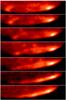 |
Fig. 1 Sequence of Brackett α acquisition images of Jupiter’s aurora. Each image was recorded just before a full UIST/IRPOL2 set of observations i.e. from the top to the bottom (UT): 0628, 0648, 0721, 0749, 0850, 0912, 0938. |
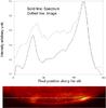 |
Fig. 2 Position of the slit on the planet, determined from matching the intensity profile of the 3.953 μm line to a cut of the brightness of the Brackett α image. UT 0721, CML 53.51. |
Acquisition images were recorded using the guide camera with the Brackett α filter in exposures of 10 s and were used to position the slit of the instrument across the main southern auroral region. The sequence of images shows the changing auroral configuration during part of the course of these observations (Fig. 1). The first (top) image and the second (immediately below) show the full southern auroral oval, displayed on the disk of the planet. The oval is strongly limb-brightened on the dusk limb due to both the oval coinciding with the limb and the fact that extends up to high altitudes, some 3000 km or more above the reference 1 bar level (Lystrup et al. 2008). Thus our line-of-sight passes through an extended column of . Poleward of the main oval, diffuse polar emission is observed to exhibit some structure, perhaps associated with the polar cap itself. As the planet rotates, subsequent images show some emission equatorward of the main oval, which will be discussed in a future publication. The offset in Jupiter’s magnetic axis (~10°) means that the auroral oval does not rotate symmetrically around the rotational pole. In the final images the auroral oval has rotated far enough that in the observer’s line of sight it is almost entirely colocated with the dusk limb. These viewing constraints must be borne in mind when interpreting the intensity profiles shown in Fig. 2 and subsequent figures.
After target acquisition, a complete UIST/IRPOL2 Jupiter observation consisted of eight exposures of 30 s each, an object and sky pair at each of the following waveplate angle positions: 0°, 22.5°, 45°, 67.5°, 90°, 112.5°, 135°, and 167.5°. These eight positions are needed to correct for spectral modulation in polarisation, which is due to multiple reflections within the plates of the wave plate assembly as described by Aitken & Hough (2001). Instrument overheads result in a total elapsed time of ~10 min to observe in all eight positions, during which Jupiter rotates ~6°. Sixteen sets of data were recorded during the night (Table 1).
Table of the 16 data sets.
Guiding was achieved using the guide camera system and was stable throughout the night. An unpolarised star (HD 188512) and a star with known polarisation in the K band (HD 150193, polarisation degree equal to 1.68 ± 0.02; angle of 60°; Whittet et al. 1992) were observed for polarisation calibration. Each set of star observations, made immediately before and after the Jupiter observations, were recorded at all eight waveplate positions.
3. Data processing
The data were reduced using the Starlink software package accounting for dark current, bad pixels, and flat-fielding1. Airmass correction, wavelength calibration, flux calibration, and sky subtraction were performed separately and the e- and o-beams in each exposure were aligned for pixel-to-pixel correspondence. The o- and e-images were both divided into 24 longitudinal bins of 6 pixels (equivalent to 0.72″) each and subtending ~1100 km on the planet.
Instrumental polarisation was not considered to be significant; according to UKIRT, it is expected to be much less than 1%. For this instrument configuration, the polarisation efficiency peaks at 97% at around 3.65 μm and falls off, approaching 86% at longer wavelengths. The efficiency as a function of wavelength (λ) has been fit by UKIRT according to P%(λ) = −398.1 + 272.6(λ) − 37.5(λ)2 and was taken into account.
This study focuses on the 3.953 μm emission line, the Q(1,0 − ) transition with ν2 → 0 (see Watson et al. 1984, for spectroscopic details). To measure the intensity of the line for each of the waveplate positions φ, we fitted the spectral profile with a Gaussian function: 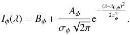 (1)We fitted the line on a group of nine pixels around the predefined line centre. To avoid local minima, a least square routine with random starting points was performed 15 times. This was only done when the 3.95 μm line was clearly identified, i.e. when the noise was far less than the signal. For data with a very low signal-to-noise ratio, the hypothesis of
  used to deduce variances of the fitted parameters becomes strongly false, and the polarisation degree has little meaning. For this reason, in cases where the emission line in our data was weak, the results become uncertain, so we do not consider these cases for the estimation of the polarisation degree.
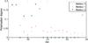 |
Fig. 3 Comparison between the polarisation degrees obtained by the three processing method for data set 5. |
3.1. Degree and angle of linear polarisation
The normalised Stokes parameters q and u are generally obtained using the ratio method (hereafter Method 1):  (2)where
  (3)In these equations, e and o refer to the intensities of the e- and o-lines at the relevant waveplate positions φ, indicated by the suffixes. They correspond to the Aφ parameters from the Gaussian fits. The same calculations give the u Stokes parameter if data for the 0° and 45° positions are replaced in the above equations by data from the 22.5° and 67.5°. This provides a calculation for the linear polarisation rate p,
  (4)and the polarisation direction θ measured counterclockwise from the slit direction:
  (5)Method 1 is subject to too much noise to be useable in deriving the degree of polarisation. Thus we considered two other methods of calculating the polarisation. The first of these (hereafter Method 2) is taken from Semel et al. (1993):
  (6)where Q and I are the non-normalised, corresponding Stokes parameters. Following Semel et al. (1993), this method is less susceptible to noise and errors. The Stokes parameter U is recovered by replacing the angles of the waveplate as in the Method 1. However, this method can give incorrect results if the waveplate retardation is not exactly 180° at 3.95 μm. A zero order waveplate presents a relative phase Γ equal to,
  (7)where L is the length of the crystal and Δn the difference in indices. In the case of UIST/IRPOL, the plate is half wave at 3.5 μm, so the retardance is expected to be 0.44 wave or 159.49° at 3.953 μm. We therefore used a third method (Method 3) that consists of solving the system of equations in Landi Degl’Innocenti et al. (2004), which gives the intensity versus the positions of the waveplate and the polariser and the retardance of the waveplate:
 ![Mathematical equation: \begin{eqnarray} D(\alpha, \beta, \delta)&=&\frac{1}{2} [I\!+\!(Q \times \cos(2\alpha) \!+\! U \times \sin(2\alpha)) \times \cos(2(\beta - \alpha)) \nonumber \\ && - \, (Q \times \sin(2\alpha)\!-\!U \times \cos(2\alpha))\sin(2(\beta - \alpha))\cos(\delta) \nonumber \\ && + \,V \times \sin(2(\beta-\alpha)) \sin(\delta)] \end{eqnarray}](/articles/aa/full_html/2011/06/aa14314-10/aa14314-10-eq65.png) (8)where α is the position of the waveplate, β is 0° for the ordinary beam and 90° for the extraordinary beam, δ is the retardance at the measured wavelength, and D the intensity at the relevant waveplate position. For example, e45 corresponds to α = 45°, β = 90°. Since we sample at eight waveplate positions, we have a system of over-determined equations that can be solved using a standard least-squares-fit procedure to derive the components of the Stokes vector. Once I, U, Q, and V are obtained, it is straightforward to calculate the normalised Stokes parameter (u, q and v) and the polarisation rate through Eq. (4).
(8)where α is the position of the waveplate, β is 0° for the ordinary beam and 90° for the extraordinary beam, δ is the retardance at the measured wavelength, and D the intensity at the relevant waveplate position. For example, e45 corresponds to α = 45°, β = 90°. Since we sample at eight waveplate positions, we have a system of over-determined equations that can be solved using a standard least-squares-fit procedure to derive the components of the Stokes vector. Once I, U, Q, and V are obtained, it is straightforward to calculate the normalised Stokes parameter (u, q and v) and the polarisation rate through Eq. (4).
Method 3 requires that the overall source intensity remains stable during the period required to measure intensities for the eight individual waveplate angles, but is the only method that accounts for the waveplate not being exactly half wave at 3.95 μm. It also has the advantage of being able to detect any circular polarisation that may be present. Gérard et al. (2003) find that no significant change in auroral emission intensity occurred during the 18 min needed to acquire FUV data (110 − 170 nm) in the main oval. This time is roughly twice that of the overall elapse time needed for our observations to cover all eight waveplate positions.
The polarisation rate calculated in Eq. (4) involves the square root of the sum of two squares, so noise on values q = 0 and u = 0 leads to a non-zero polarisation rate. This problem has been treated by Simmons & Stewart (1985), who proposed several debiased estimators. The maximum likelihood estimator is most accurate in the case of low signal-to-noise ratios. This estimator is the value of the polarisation rate p0 which maximises the Rice distribution for polarisation:  (9)where J0 is the zeroth-order Bessel function, p is the biased estimator divided by its uncertainty, and p0 the true polarisation rate. The unbiaised polarisation pc rate is given by
  (10)This estimator results in a threshold at p = 1.41 (i.e. when the ratio
  ), below which we are unable to identify polarisation with any certainty. Bins for which p = 1.41 are assigned a polarisation rate of zero and polarisation angles for these bins are not included in the figures presented here.
To test and choose the best method, we ran the three method on a panel of data sets. As expected, Method 1 is sensitive to noise. In our data, it seems that Method 2 is also sensitive, giving some unexplained variation in the polarisation rate. To check that Method 3 is less sensitive to noise than the others, we compared several data sets for the pattern of the polarisation rate for the three methods (Fig. 3). We can see that Method 3 is the method with generally the lowest polarisation rate, justifying the choice of this method for polarisation detection; for example, for the dataset 5, Method 3 gives lower polarisation rates except for 1 point.
Finally, to check the consistency of our results, we obtained the intensities of the line in the different spectra by summing the intensities over nine individual pixels around the line centre, rather than by fitting a Gaussian profile to the line and integrating. The polarisation measurements derived from both the Gaussian profiles and the pixel-summation profiles match well, although the latter are noisier.
3.2. Reference stars
For the reference stars, the polarisation direction is taken from the celestial local meridian to allow comparison with tabulated values. The spectrum of the unpolarised standard HD 188512 produced a polarisation of 0.95 ± 0.04% for the 100 pixels around 3.95 μm, with a polarisation angle of 67° ± 2°. The polarised standard HD 150193 produced a polarisation degree of 1.53 ± 0.05% with an angle of 66° ± 2° for the 100 pixels surrounding 3.95 μm. These polarisation rates are higher than expected, particularly for the unpolarised standard. For the polarised standard, we can extrapolate the power law of Whittet (Whittet et al. 1992) using polarisation rates in the U, B, V, R, I, J, H, K bands to 4 μm. This gives a polarisation around 0.5%. Since the anticipated instrumental polarisation is less than 1%, however, the 0.95% found for the unpolarised star is consistent with a value of zero, and that of the polarised standard with its extrapololated value of 05.%. Nonetheless, given the uncertainty over the stellar calibrations and the instrumental contribution, we consider that polarisation rates of less than 1.5% in our data are unreliable. As far as the angles are concerned, the polarisation angle seems to increase with the wavelength for our polarised star (θ(H band) = 57°, θ(K band) = 60°, (Whittet et al. 1992). The value of 66° ± 2° that we derive can be considered consistent with this trend and as a reliable reference for calibrating polarisation angles for our Jovian spectra.
3.3. Slit position determination
The Brackett-α acquisition images obtained prior to each set of spectro-polarimetry observations can be used to gauge the position of the slit projection on the planet during the observations. To do this, the wavelength profile of the emission line at 3.953 μm was first fitted with a Gaussian, and the peak intensity at each pixel along the slit was used to create a spectral intensity profile. This was compared to image brightness profiles of east-west cuts through the Brackett α image at different latitudes, and the slit latitude was then taken as being the one for which the best match was found between the image and spectral intensity profiles. An example is shown in Fig. 2.
Both the spectral profile (solid line) and the image profile (dotted line) in Fig. 2 show a number of features in common. In the profiles and the accompanying image, planetary west (dawn) is on the left, and planetary east (dusk) is on the right. We have labelled five regions from left to right as the west oval exterior (WOE), the west oval interior (WOI), the polar regions (PR), the east oval interior (EOI) and the east oval exterior EOE). The WOE represents a region from the limb of the planet to the peak of the dawn auroral oval. The spectrometer slit is sampling magnetic latitudes below that of the main auroral oval up to the oval itself. The intensity rises more or less monotonically with increasing magnetic latitude, although in Fig. 2 there is some indication in both the spectral and image profiles of a subauroral arc or spot. The WOI represents the slit projecting from the main auroral oval polewards. Here the intensity decreases sharply with increasing magnetic latitude, to reach a minumum on the western side of the PR. Through the PR the intensity increases slowly from west to east, before rising rapidly in EOI to the peak of the dusk auroral oval. Finally, the intensity decreases rapidly in the EOE from the peak of the main auroral oval to the dusk limb of the planet.
Our technique of profile matching does not provide an exact match between the spectral and image intensity profiles for a number of reasons. First, there is a short timelag between the acquisitions of the image and that of the spectra, that results in the central meridian longitudes being slightly different. Thus the profiles are intrinsically sampling slightly different views of the planet. Second, the spectra have higher wavelength resolution than the images. This results in a more intense continuum background contribution in the image profiles than in the spectral profiles. This background comes from thermal emission from Jupiter’s lower atmosphere, as well as from some reflected solar infrared radiation, neither of which has the same east-west spatial morphology as the upper atmosphere auroral emission. Finally, insofar as the Brackett-α emission is auroral, it is produced from H atoms, whose altitude distribution is very different from that of : H atoms dominate at higher altitudes than the H2 molecules that gives rise to , so H is sensitive to excitation by lower energy electrons (probably with energies < 10 keV). Again, the exact location where these lower energy electrons deposit their energy does not have to match where the higher energy electrons (10 − 60 keV) produce emission. Because of these differences, the main criterion for determining the best estimated latitude makes use of the positions of the eastern and western auroral peaks. We define the effective latitude of the observations as the one for which the best match between the spectral profile peaks and the image profile peaks is obtained.
4. Results
In the first eight data sets, the intensity profiles show two peaks corresponding to locations where the slit projection on the planet crosses the dawnward and duskward main auroral oval, similar to those shown in Fig. 2. The last eight sets of data, acquired 40 min later, show only one peak, corresponding to a duskward oval crossing. By that time the oval had rotated to Jupiter’s dusk-side. The main oval is still visible, but line-of-sight effects cause difficulty in distinguishing it from other high-latitude structures. For this reason, and also because the signal-to-noise ratio of the emission line intensity is better in the first group, we only consider the first eight data sets in this study. Not surprisingly, the best signal-to-noise ratio appears in bins where the intensity of the auroral emission is highest.
4.1. Linear polarisation
We present results only for data bins for which the signal-to-noise ratio for the intensity of the 3.953 μm emission line is greater than 7 so that resulting intensity ratios at the various waveplate positions would have S/N > 3. We also used a χ-squared test and eliminated all points with reduced χ2 greater than 2.26 in order to eliminate false fit results. This corresponds to a level of confidence of 95.4% that the fit is false.
This procedure has a threshold effect, so polarisation is most clearly present in bins where the signal is stronger, i.e. in the main oval. That means a negative report does not imply that polarisation is not present, but simply that our criteria for reporting it have not been met.
Some values of the polarisation parameters for Datasets 1, 2, 5, and 8 are given in Figs. 4 to 7 with 1σ error bars, for which at least some bins met our reporting criteria. The highest unambiguous measured polarisation rate is 6.63 ± 1.48% (8th data set, bin 24). Polarisation detections with confidence levels superior to 3σ are listed in Table 2.
Polarisation detections with a confidence level superior to 3σ.
4.2. Circular polarisation
The normalised Stokes v parameters has also been calculated. Several points with circular polarisation appear with confidence level higher than 3σ. Both left and right polarisation are present, but the negative (right) v values are greater than the left ones. The highest absolute value of v is 0.34 in a right configuration. This is particularly important, and it validates a posteriori the method we used to calculate the Stokes parameters.
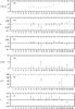 |
Fig. 4 Results for the first data set, recorded at 6:19 UT. Error bars indicate the 1σ confidence level. a) Intensity of the 3.95 μm line in arbitrary unit. Missing values correspond to points where the Gaussian fits were not satisfactory. b) Normalised Stokes parameter q. c) Normalised Stokes parameter u. d) Debiased polarisation rate pc. e) Polarisation angle θ where pc ≠ 0. 90° corresponds to a vertical polarisation vector; 0° corresponds to an horizontal vector on the Jovian disk (i.e. referring to the slit direction). f) Normalised Stokes parameter v. |
5. Discussion
5.1. Linear polarisation
Although we have unambiguously detected a measurable degree of polarisation in the Jovian auroral and polar emissions, our results do not demonstrate any clear correlation between the degree of polarisation and the location on the main oval. There is some evidence that the highest reportable levels are for pixels just to the east of the main oval for data sets 1, 2, and 8.
Polarisation direction along the slit, taken from the slit direction in the trigonometric sense in degree.
Polarisation angles are fairly unstructured. They are listed in Table 3. The exterior part of the west oval presents only two accurate points. Polarisation angles are around 100° from the slit in the direction of the trigonometric rotation. The interior region shows angles that are more or less parallel to the slit with angles around 150° for data sets 3, 4, and 5 and between 0° and 25° for the three subsequent sets. In the polar regions we found no preferential direction. The east oval presents directions around 90°(between 60° and 120°) in its inner region and direction parallel to the slit in its exterior region (between 170° and 8°). It is difficult to interpret this direction because there is currently no theoretical link between the polarisation and the local fields. The complex and small-scale structure of the polar region validates the difficulty of finding a preferential direction in this region. Besides that, the FUV intensity of the emissions can vary on timescales of tens of seconds in the PR (Gérard et al. 2003). The method we used is not valid in the PR if such rapid variations occur in emission there.
5.2. Circular polarisation
We also observed circular polarisation, which is more difficult to interpret than the linear polarisation. The sign of the Stokes v parameter seems to be strongly structured (Table 4). For those cases where we are confident of the detection, the EOE always shows a negative value of v and the EOI a positive one. The PR does not show a clear structure, and the circular polarisation is often close to zero. For the west oval, the WOE presents a positive Stokes v value and the interior region a negative one, except for the first two data sets.
Sign of the Stokes v normalised parameter along the slit.
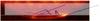 |
Fig. 8 Polarisation direction for data set 8, overlayed on the disk recorded at 7:49 UT. The length of the vector represents the polarisation degree. |
5.3. Possible links with the E and B fields
There may be several processes causing the molecular anisotropy that results in the observed polarisation. The ionospheric electric field has an effect on the polarisability tensor of the molecule. This results in a small additional dipole being generated parallel to the electric field, which adds to the dipole associated with the ν2 ro-vibrational transitions being observed. There are no direct measurements of the ionospheric field although, as previously mentioned, but it may be deduced from calculations (Smith et al. 2005). Generally, the electric field is thought to be directed equatorwards across the main auroral oval. If the electric field is the primary factor affecting the observed polarisation, then the angle would be expected to be 165° at the dawn limb. In the dusk sector of the oval, the angle should be 15° at the limb. On the body of the planet, the polarisation angle would gradually approach 90° towards the centre. However, superimposing the polarisation direction on the Bracket α image (Fig. 8) does not fit well with these expectations. That said, the spatial variability of auroral processes and the corresponding electric fields generated in the ionosphere (Smith et al. 2005; Lystrup et al. 2007) may explain that no clear link between the polarisation and the fields appears in these first observations. The circular polarisation, on the other hand, seems to be more structured than the linear one.
Proper interpretation of these results requires full ab initio calculations and laboratory experiments concerning the polarisation of emission, work that has not yet been performed. Initial calculations show that changes in the computed Einstein A coefficients of the lines observed in this study can be generated by including a small fixed dipole in the space-fixed x-direction, which could correspond to north-south on the planet. For the Q(1,0 − ) line at 3.953 μm, a fixed dipole of just 0.01 atomic units (0.025 Debye) causes a reduction in A from 129 s-1 to 113 s-1, of about 12.5% and more than enough to account for our observed polarisation.
Notwithstanding our current inability to model it fully, the detection of polarisation in the emission from Jupiter’s auroral/polar regions gives planetary scientists another tool with which to probe the physical conditions of upper atmospheres. The polarisation of other lines could also be studied. For example, the auroral Lyman α line could be polarised, and the Stokes parameters can be linked with the magnetic field due to Hanle effect during radiative transfer (Ben-Jaffel et al. 2005) and also with the particle precipitation energy (James et al. 1998). If those theoretical effects are confirmed, it seems that, as in the case for the Earth, simultaneous polarisation observations of several emission lines could help determine prevailing ionospheric conditions and thus provide constraints for ionospheric models.
6. Conclusions
We have reported the first measurement of polarisation in infrared Jovian auroral emissions with a confidence level greater than 3σ for both linear and circular polarisation. These results were found under the assumption that the emission intensity is constant during each set of observations, which is true in the main oval following Gérard et al. (2003). The polarisation appears primarily in or close to the main auroral oval, with polarisation degrees up to 7%. Polarisation directions are unstructured, and there appears to be no definitive link with local anisotropy. However, a structured circular polarisation is measured. Laboratory experiments and ab initio calculations are now needed to fully understand these results. For now, follow-up observations to confirm detections in the northern and southern aurora with better signal-to-noise ratios are not possible. The spectro-polarimetry instrument on UKIRT was the only facility capable of making these measurements owing to the required wavelength range and resolution, and since the time of these observations the telescope has ended the use of its Cassegrain instruments. Other emission lines could be polarised in the Jovian auroral emissions, especially the Lyman α line and the H2 Werner and Lyman bands. Such observations would require a FUV spectro-polarimeter, not currently in existence.
Details of the Starlink software package are available at http://starlink.jach.hawaii.edu/
Acknowledgments
We thank Chris Davis and Tim Carroll for their expert assistance during these observations. The United Kingdom Infrared Telescope is operated by the Joint Astronomy Centre on behalf of the Science and Technology Facilities Council of the UK We thank the Department of Physical Sciences, University of Hertfordshire, for providing IRPOL2 for the UKIRT. We thank Veronique Bommier and Herve Lamy for useful discussions. We thank Renee Prange for helping to initiate this collaboration. M. B. Lystrup is supported by an NSF Astronomy and Astrophysics Postdoctoral Fellowship under award AST-0802021. U.G. and U.C.L. are part of the Europlanet RI, the European planetary science network, which is supported by the European Union’s Framework 7 programme.
References
- Aitken, D. K., & Hough, J. H. 2001, PASP, 113, 1300 [NASA ADS] [CrossRef] [Google Scholar]
- Ben-Jaffel, L., Harris, W., Bommier, V., et al. 2005, Icarus, 178, 297 [NASA ADS] [CrossRef] [Google Scholar]
- Bommier, V., Sahal-Bréchot, S., Dubau, J., & Cornille, M. 2011, Ann. Geophys., 29, 71 [Google Scholar]
- Gérard, J., Gustin, J., Grodent, D., Clarke, J. T., & Grard, A. 2003, J. Geophys. Res., Space Phys., 108, 1319 [CrossRef] [Google Scholar]
- James, G. K., Slevin, J. A., Dziczek, D., McConkey, J. W., & Bray, I. 1998, Phys. Rev. A, 57, 1787 [NASA ADS] [CrossRef] [Google Scholar]
- Landi Degl’Innocenti, E., & Landolfi, M. 2004, Polarization in Spectral Lines (Dordrecht: Kluwer Academic Publishers), Astrophys. Space Sci. Libr., 307 [Google Scholar]
- Lilensten, J., Moen, J., Barthélemy, M., et al. 2008, Geophys. Res. Lett., 35, 8804 [Google Scholar]
- Lystrup, M. B., Miller, S., Stallard, T., Smith, C. G. A., & Aylward, A. 2007, Ann. Geophys., 25, 847 [NASA ADS] [CrossRef] [Google Scholar]
- Lystrup, M. B., Miller, S., Dello Russo, N., Vervack, Jr., R. J., & Stallard, T. 2008, ApJ, 677, 790 [NASA ADS] [CrossRef] [Google Scholar]
- Miller, S., Achilleos, N., Ballester, G. E., et al. 2000, Roy. Soc. Lond. Phil. Trans. Ser. A, 358, 2485 [Google Scholar]
- Rego, D., Achilleos, N., Stallard, T., et al. 1999, Nature, 399, 121 [NASA ADS] [CrossRef] [Google Scholar]
- Semel, M., Donati, J., & Rees, D. E. 1993, A&A, 278, 231 [NASA ADS] [Google Scholar]
- Simmons, J. F. L., & Stewart, B. G. 1985, A&A, 142, 100 [NASA ADS] [Google Scholar]
- Smith, C. G. A., Miller, S., & Aylward, A. D. 2005, Ann. Geophys., 23, 1943 [NASA ADS] [CrossRef] [Google Scholar]
- Watson, J. K. G., Foster, S. C., McKellar, A. R. W., et al. 1984, Can. J. Phys., 62, 1875 [NASA ADS] [CrossRef] [Google Scholar]
- Whittet, D. C. B., Martin, P. G., Hough, J. H., et al. 1992, ApJ, 386, 562 [NASA ADS] [CrossRef] [Google Scholar]
All Tables
Polarisation direction along the slit, taken from the slit direction in the trigonometric sense in degree.
All Figures
|
Fig. 1 Sequence of Brackett α acquisition images of Jupiter’s aurora. Each image was recorded just before a full UIST/IRPOL2 set of observations i.e. from the top to the bottom (UT): 0628, 0648, 0721, 0749, 0850, 0912, 0938. |
| In the text | |
|
Fig. 2 Position of the slit on the planet, determined from matching the intensity profile of the 3.953 μm line to a cut of the brightness of the Brackett α image. UT 0721, CML 53.51. |
| In the text | |
|
Fig. 3 Comparison between the polarisation degrees obtained by the three processing method for data set 5. |
| In the text | |
|
Fig. 4 Results for the first data set, recorded at 6:19 UT. Error bars indicate the 1σ confidence level. a) Intensity of the 3.95 μm line in arbitrary unit. Missing values correspond to points where the Gaussian fits were not satisfactory. b) Normalised Stokes parameter q. c) Normalised Stokes parameter u. d) Debiased polarisation rate pc. e) Polarisation angle θ where pc ≠ 0. 90° corresponds to a vertical polarisation vector; 0° corresponds to an horizontal vector on the Jovian disk (i.e. referring to the slit direction). f) Normalised Stokes parameter v. |
| In the text | |
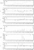 |
Fig. 5 Same as Fig. 4 for data set 2, recorded at 6:29 UT. |
| In the text | |
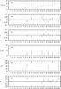 |
Fig. 6 Same as Fig. 4 for data set 5, recorded at 6:38 UT. |
| In the text | |
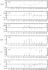 |
Fig. 7 Same as Fig. 4 for data set 8, recorded at 7:39 UT. |
| In the text | |
|
Fig. 8 Polarisation direction for data set 8, overlayed on the disk recorded at 7:49 UT. The length of the vector represents the polarisation degree. |
| In the text | |
Current usage metrics show cumulative count of Article Views (full-text article views including HTML views, PDF and ePub downloads, according to the available data) and Abstracts Views on Vision4Press platform.
Data correspond to usage on the plateform after 2015. The current usage metrics is available 48-96 hours after online publication and is updated daily on week days.
Initial download of the metrics may take a while.