| Issue |
A&A
Volume 529, May 2011
|
|
|---|---|---|
| Article Number | A13 | |
| Number of page(s) | 13 | |
| Section | Cosmology (including clusters of galaxies) | |
| DOI | https://doi.org/10.1051/0004-6361/200913918 | |
| Published online | 21 March 2011 | |
Magnetic power spectra from Faraday rotation maps
REALMAF and its use on Hydra A
Max Planck Institute for Astrophysics, Karl-Schwartzschildstr.1, 85741 Garching, Germany
e-mail: This email address is being protected from spambots. You need JavaScript enabled to view it.
Received: 19 December 2009
Accepted: 29 January 2011
Abstract
We develop a novel maximum-a-posteriori method to measure magnetic power spectra from Faraday rotation data and implement it in the REALMAF code. A sophisticated model for the magnetic autocorrelation in real space permits us to alleviate previously required simplifying assumptions in the processing. We also introduce a way to treat the divergence relation of the magnetic field with a multiplicative factor in Fourier space, with which we can model the magnetic autocorrelation as a spherically symmetric function. Applied to the dataset of Hydra A north, we find a power law power spectrum on spatial scales between 0.3 kpc and 8 kpc, with no visible turnover at large scales within this range and a spectral index consistent with a Kolmogorov-like power law regime. The magnetic field strength profile seems to follow the electron density profile with an index α = 1. A variation of α from 0.5 to 1.5 would lead to a spectral index between 1.55 and 2.05. The extrapolated magnetic field strength in the cluster centre highly depends on the assumed projection angle of the jet. For an angle of 45° we derive extrapolated 36 μG in the centre and directly probed 16 μG at 50 kpc radius.
Key words: magnetic fields / galaxies: clusters: intracluster medium / radio continuum: general / polarization / turbulence / plasmas
© ESO, 2011
1. Introduction
1.1. Motivation
Intergalactic magnetic fields are of great scientific interest. They are part of the intergalactic metabolism, they affect the propagation of heat and cosmic rays, and they are tracers of the dynamical state of the intergalactic medium. One way to retrieve their properties is to measure the Faraday rotation effect they cause on traversing polarised light. This has lead to significant insight into the presence, strength, and morphology of magnetic fields in galaxy clusters.
Although it is not possible to retrieve the exact magnetic field in position space from Faraday rotation data, the magnetic power spectrum is accessible and contains information on the typical field strength, correlation length, and the distribution of magnetic energy onto different length-scales. All these quantities can be predicted in magneto-genesis theories. The latter, the spectral energy distribution, is a sort of fingerprint of these theories. Magneto-genesis-scenarios in which the energy is injected on large scales by gas stirring typically exhibit Kolmogorov-like power law spectra (Subramanian et al. 2006; Enßlin & Vogt 2006). Whereas scenarios in which the magnetic fields are built up from small to large scales typically exhibit different spectral slopes (Schekochihin & Cowley 2006). Magnetic field measurements by Faraday rotation therefore have the potential to distinguish between these theories.
1.2. Faraday rotation
The plane of polarisation of light traveling to us through a magnetised plasma is changed by the wavelength-dependent Faraday rotation effect. If the Faraday rotating plasma is entirely located between the radio source (at physical depth zs and at position x ⊥ in the plane of sky) and the observer (assumed to be at z = ∞), the effect is a plain change of the original polarisation angle χ0 according to 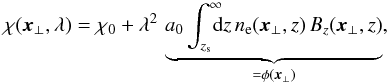 (1)with a proportionality constant
  , with c, e, and me being the speed of light, the electron charge, and the mass, respectively. Furthermore, ne(x) and B(x) are the electron density and the magnetic field within the Faraday rotating foreground medium, and φ(x ⊥ ) denotes the Faraday depth of the source at x ⊥ . Although the original polarisation angle χ0 is unknown, measurements of the polarisation angle at a range of wavelengths λ provide this observationally, and also an estimator of the Faraday depth φ via a fit to Eq. (1). The observational estimate of the Faraday depth is called the rotation measure (RM), because it expresses the rate at which the linear polarisation rotates as a function of λ2.
Some of the many studies of magnetic fields via Faraday rotation are Dennison (1979), Lawler & Dennison (1982), Dreher et al. (1987), Laing (1988), Hennessy et al. (1989), Taylor et al. (1990), Goldshmidt & Rephaeli (1993), Kim et al. (1991), Ge & Owen (1994), Feretti et al. (1995), Johnson et al. (1995), Johnson et al. (1995), Feretti et al. (1999a,b), Clarke et al. (2001), Taylor et al. (2001), Carilli & Taylor (2002), Taylor et al. (2002), Eilek & Owen (2002), Murgia et al. (2004), Laing et al. (2006), Xu et al. (2006), Taylor et al. (2007), Cho & Ryu (2009), Feain et al. (2009), and Battaglia et al. (2009), where we omitted works directly addressed in the following.
1.3. REALMAF
In this work, we present the code REALMAF (REAL MAgnetic Fields), which is aimed at measuring magnetic power spectra in galaxy clusters from maps of Faraday rotation measurements and apply this code to the Hydra A cluster.
As will be detailed in the following sections, our method relies on these informations and assumptions:
-
the linearity of the measurement process (seeSect. 2.1);
-
the maps of rotation measures and their errors (see Sect. 4.1);
-
knowledge of the geometry of the Faraday active volume, which also depends on the projection angle θ of the jet and the cavity size (see Sect. 4.2);
-
assuming that there is no polarised radio emission inside the Faraday active volume in front of the radio bubble (see Sect. 4.2);
-
knowledge of the electron density profile ne of the cluster atmosphere (see Sect. 4.2);
-
assuming that the magnetic field strength B follows the electron density profile like
 (e.g. Dolag et al. 2001,and see Sect. 3.4);
 -
assuming Gaussian probability distributions for the magnetic fields and the measurement errors in the rotation measure map (see Sect. 2.2);
-
assuming statistical isotropy of B (see Sect. 2.3);
-
assuming solenoidal fields (see Sect. 2.3);
-
using a Bayesian approach to inference with a scale-independent prior for the power spectrum (see Sect. 3.1).
We use H0 = 70 km s-1 Mpc-1, Ωm = 0.3, ΩΛ = 0.7 and a redshift of 0.0538 for Hydra A (de Vaucouleurs et al. 1991), which gives a linear to angular conversion factor 1′′ = 1.047 kpc. To follow the tradition in cosmic magnetism studies, we use cgs-units in this paper with the energy unit 1 erg = 10-7 J and magnetic field strength unit 1 G = 10-4 T.
2. Magnetic field statistics in Faraday screens
2.1. Measurement equation
The rotation measure differs from the Faraday depth as defined by Eq. (1) only by the measurement noise n:  (2)We assume the signal-to-noise ratio of the polarised flux to be sufficiently high for an accurate RM determination within an area A in the sky. The n-tuple of the RM values there then forms our data vector d = (RM(x ⊥ ))x ⊥ ∈ A, from which all deductions will be made. The RM data can be regarded as the result of a functional linear response operator R acting on the three-dimensional magnetic field configuration and producing a two-dimensional sky image of it,
  (3)where the elements of the response matrix R are defined in Eq. (2) and the application of R on B should be read as the index-sum and line-of-sight integration given in the same equation. The extended Faraday effect in the intra-cluster medium in front of the Hydra A radio galaxy was accurately measured by Taylor & Perley (1993). The intra-cluster medium has a roughly spherical symmetric electron density ne(x ⊥ ,z) centred on the Hydra A cD galaxy. The radio jets of Hydra A inflate bubbles with relativistic, radio emitting plasma, which are visible as cavities in the X-ray emission of the surrounding hot cluster atmosphere (Wise et al. 2007). On its way to the observer the polarised radio emission of these bubbles experiences a rotation of its polarisation plane because of the Faraday effect of the magnetised intra-cluster medium.
2.2. Gaussian random fields
Owing to the information lost in the projection, Eqs. (2) and (3) are not directly invertible. It is therefore impossible to calculate the line-of-sight magnetic field Bz from φ and the known electron density profile. However, we will see that assuming statistical isotropy of the magnetic fields and using a statistical approach we are able to retrieve the amplitude spectrum of the magnetic field in Fourier space, the magnetic power spectrum  , and the typical field strength B in position space and its autocorrelation length λB, which are determined by ω(k). The expectation brackets should be understood as an average over the ensemble of possible magnetic field configurations produced by typical intra-cluster dynamics. We will assume that the magnetic field statistics generated by those is Gaussian.
Gaussian magnetic fields statistics is not what numerical simulations of MHD turbulence find, see Waelkens et al. (2009). However, they are the starting point of any analysis of correlation functions. If all we know statistically about the fields is their two-point correlation, the assumption which only expresses this knowledge is a Gaussian of which this correlation matrix is the covariance matrix. Any other distribution function would contain more information in a Shannon-Boltzmann sense.
Before we can gain additional information on higher order statistics, we need to understand more the two point correlation function, and this is possible even with an approximate assumption on the statistics. Non-Gaussianities could modify the result of a power spectrum measurement based on the assumption of Gaussian fields. However, this modification can be expected to be of a modest nature, much smaller than the systematic uncertainties we deal with because of the imperfect modeling of the galaxy cluster’s atmosphere structure and the geometry of the radio source that was used to probe for Faraday rotation. Our method is relatively robust to non-Gaussian modifications, because the observational quantities it exploits, the product of RM values at different locations, are a linear transformation of the magnetic two-point correlation, irrespective of whether the underlying magnetic field statistics are Gaussian or not.
Finally, many other methods also use Gaussian random fields or assume them implicitly, e.g. Murgia et al. (2004); Bonafede et al. (2010a,b); Vacca et al. (2010); Govoni et al. (2010).
Using again the functional vector notation, we can write the Gaussian probability to find a magnetic field configuration B given a magnetic covariance matrix M = ⟨ B BT ⟩ , with elements Mij(x,y) = ⟨ Bi(x) Bj(y) ⟩ : 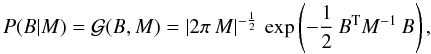 (4)with | M | being the determinant of the magnetic covariance matrix.
2.3. Magnetic correlation tensor
If there is a statistical translation invariance, Mij(x,y) depends only on the distance x − y because the absolute position cannot matter and only relative positions determine the two-point statistics. As a consequence, the magnetic covariance matrix becomes diagonal in its Fourier space representation with respect to the k-vector: 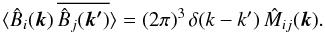 (5)If we deal with statistical isotropy, one moreover finds for solenoidal fields (∇·B = 0)
 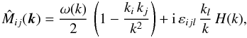 (6)(see e.g. Subramanian 1999; Enßlin & Vogt 2003) and therefore
 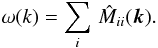 (7)H(k) specifies the magnetic helicity, which does not play any role in this work, because it does not lead to any detectable signature in Faraday rotation maps alone, as we will see shortly.
2.4. Faraday statistics
Assuming Gaussian statistics for turbulent magnetic fields has the pleasant property that the probability function of the Faraday depth φ is also Gaussian: 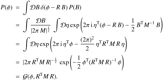 (8)Here, we used the Fourier representation of the Dirac delta function (in functional spaces) as well as the well known property of Gaussian integrals
  , which also holds for functional or path integrals denoted by
  . The φ-covariance Cφ = ⟨ φ φT ⟩ = RTM R reads for our specific response and magnetic covariance matrices
 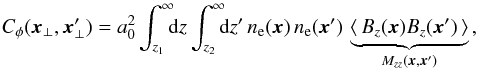 (9)where z1 and z2 denote the depth to the surface of the radio source at sky position x ⊥ and
  , respectively. If the spatial electron distribution is constant, the magnetic fields are statistically homogeneous and isotropic and the observation samples a virtually infinitely extended Faraday active volume, this can be simplified even more, and reads in Fourier space
 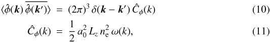 where Lz is the depth of the Faraday screen. Thus, clearly the magnetic energy, but not the helicity spectrum can be retrieved from Faraday rotation maps. In the more realistic case the geometry is less simple (finite observed volume, structured electron density, and magnetic field strength profiles, etc.). This formula has to be replaced by one which takes these effects into account, as derived in Enßlin & Vogt (2003). Because then the different Fourier modes couple, it can become simpler to again work in the position space, as we will do below (see Sect. 3.4).
2.5. REALMAF and other power spectra estimators
We model the magnetic power spectrum as a combination of spectral basis functions 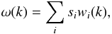 (12)where the spectral amplitudes form our spectral signal s = (si). The number of bins, and therefore the number of free parameters of our inference problem, will be set by a trade-off between the aim to have high spectral resolution and to have small and uncorrelated vertical error bars in the spectrum1.
A probability function for s given the data d, the posterior P(s | d), will be set up later in this work in Sect. 3.2. Maximising the posterior with respect to the parameters in s provides an estimator for ω(k) expressed as amplitudes of relatively independent frequency bands. A similar approach has already been applied to the Hydra A cluster by Vogt & Enßlin (2005). Expressing the spectral basis functions as analogous basis functions for the magnetic autocorrelation allows us to calculate the RM covariance matrix completely in position space, which makes two rough simplifications in the processing used by Vogt & Enßlin (2005) unnecessary (see Sect. 5 for further discussion). Moreover we include noise effects into the analysis and model the Faraday screen more accurately using recently improved measurements of the geometry of the cavities in the Hydra A cluster by Wise et al. (2007).
The Hydra A cluster has been investigated by Laing et al. (2008) as well. They compared simulated rotation measure structure functions with the observed ones. A comparison with their results will be discussed in Sect. 5.
Another approach for retrieving magnetic power spectra is the one proposed by Murgia et al. (2004). Assuming a power law power spectrum, they simulated Faraday rotation maps by using the FARADAY code and compared the observed and synthetic profiles of the dispersion of the RM as fit criterion. In order to find a good fit, Murgia et al. (2004) assumed a power law to restrict the number of degrees of freedom. This method was also applied e.g. by Govoni et al. (2006) and Guidetti et al. (2008).
The REALMAF code presented in this work should alleviate several of the restrictions and assumptions of former approaches. Although REALMAF also requires the spectral range to be set up by hand, the posterior statistic calculated by it guides the choice. The power spectrum within the chosen range is relatively free to adopt any slope required by the data and permitted by the number of assumed spectral bands.
3. Inference method
3.1. Statistical inference and frequentist estimates
In this work concepts from statistical inference will be applied to Faraday rotation data to measure magnetic field properties. Because this is traditionally done via frequentist estimates, we here briefly recall the conceptual differences in the methods.
In a traditional frequentist data analysis the question is asked how likely the data would have emerged under certain model parameters, in the following called the signal. The parameters or signal values with high likelihood are then favoured over the ones with low likelihood. The likelihood is often estimated by comparing a statistical summary of the real data with that of simulated mock data sets and by characterising their similarity and difference. In our case the Faraday rotation dispersion and empirical correlation functions are typically used as statistical summaries of the RM data. A comparison of data and model seems to be transparent, because it happens completely in data space. One can easily inspect the mock data by eye and compare them to the real one. This is one reason why frequentist methods are popular. Another one is their lower computational complexity, because they usually only require calculating the measurement process in a forward fashion.
In statistical inference, a different question is addressed: How probable is a signal or a model given the data and other information sources? This is the reverse from the frequentist question and is actually the more relevant question scientifically. Answering it requires some knowledge or assumption on how probable the model was before taking the data. This prior probability, in combination with the likelihood probability, permits us – using the Bayes theorem – to construct the posterior probability of a model given the data and any earlier knowledge, which then answers the question. Because this deduction takes the reverse causal way of the measurement process, the computational complexity is usually higher than that of a comparable frequentist method.
Thus, the statistical inference (or the Bayesian) approach is more abstract in trying to do deductions in the model or signal space. Its answer is a probability function in model space and not a single estimate. The mean and variance of the posterior are often used to characterise the solution. And no mock data and statistical summaries are usually generated, because the inference inserts the observed data into a likelihood function from which a backward deduction of the model is done.
Frequentist and Bayesian results often agree. However, there are at least three reasons why they can differ, and we believe that the latter two matter here:
-
1.
Bayesian methods specify the prior assumptions explicitely,while those are often implicit in frequentist estimates. Becausethe prior has some impact on the result, different choices of priorswill lead to different results.
-
2.
Bayesian methods are better suited to exploit the full information content of the data. The summary statistics used in frequentist analysis often looses a significant amount of the information imprinted in the data. In our case, we are investigating the correlation between all pairs of pixels, but a typical frequentist statistics might only look at the variance of the individual pixels or the correlation function from a subset of similar pixels, and therefore exploits much less of the data complexity.
-
3.
There are situations where no suitable summary statistics exist to construct an empirical likelihood. In our case, calculating an empirical RM correlation function to compare data with mock data only makes sense if the RM field can be assumed to result from a statistically homogeneous process. However, we are facing a very inhomogeneous geometry here because of the highly structured cluster atmosphere, with very few comparable lines of sight. How to obtain a meaningful two-point correlation function from the data in this situation is not clear to us.
Because of the last point, the Bayesian inference performed in this work does not provide common quantities of frequentist analysis like mock data, observed RM correlation function, and the like. The RM data are confronted with the theoretical covariance matrix that is expected for a given power spectrum of the magnetic field after a model of the inhomogeneous cluster atmosphere is factored out. The power spectrum would, in a statistically homogeneous setting, describe an easily observable RM correlation function, but not in our inhomogeneous case.
The Bayesian approach also extracts statistical information from poorly sampled quantities, while providing the correct large uncertainty resulting from the undersampling. For example in our case the magnetic modes on scales of or larger than the observed RM map are clearly undersampled. The largest modes appear as a single number in the data, the mean RM value of the map. Because it is a single number, it is hard to invert this into precise spectral information on large-scale magnetic fluctuations. Nevertheless, there is some useful information in this number, especially if it is far from zero. In this case, the total magnetic spectral power on large spatial scales should be on a level which makes the observed mean RM value sufficiently likely. The use of a Jeffreys prior on all spectral amplitudes enforces in our application that the inversion of poorly constrained modes is made in a very conservative fashion. With frequentist methods the usage of the information in such poorly sampled modes is more difficult, because no empirical statistics can be built up from a single observation.
3.2. Statistical basics
Our aim is to retrieve from the rotation measures (data d) the magnetic power spectrum represented by the spectral amplitudes (signal s). The Bayes theorem expresses the posterior P(s | d) (the conditional probability of the signal given the data) in terms of the likelihood P(d | s) in the following way:  (13)Because P(d) is a constant with respect to s, the most probable s given d can be retrieved by maximising the joint probability, which consists of the likelihood P(d | s) multiplied with the prior P(s). These will be specified now for our problem.
In our case the signal is the ensemble of spectral amplitudes s = (si)i. We adopt Jeffreys prior for each spectral amplitude, so that  . Jeffreys prior is a uniform distribution on a logarithmic scale, expressing that we are beforehand not even sure about the magnitude of the magnetic spectrum.
Our likelihood P(d | s) has to incorporate two stochastic processes. The first is the realisation of the magnetic field configuration according to Eq. (4). Because s fully determines the here relevant symmetric part of the magnetic correlation tensor, M = M(ω,H) = M(∑ isi ωi,H), the statistics of the Faraday depth is determined by it as well, and it is also Gaussian according to Eq. (8). If the noise is also Gaussian, then the data are Gaussian with a covariance matrix C, with entries Cij = ⟨ di dj ⟩ for the correlation of RM data at locations x ⊥ ,i and x ⊥ ,j. Using vector and matrix notation for the data vector d = φ + n and its covariance matrix C, we can write the Gaussian as  (14)An expression for C as a function of our spectral parameter s is needed. In the view of the linearity of Eq. (2), the observed data RM can be expressed in terms of the magnetic field B (vector over physical space), a response matrix R (projecting from physical to data space) and noise n (in data space) as: d = R B + n. From this we find
 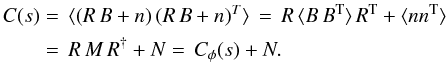 Thus to any derived Faraday rotation covariance matrix Cφ = ⟨ φ φT ⟩ an estimate for the noise covariance matrix N = ⟨ nnT ⟩ needs to be added.
3.3. Maximising the posterior
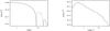 |
Fig. 1 Left: the magnetic autocorrelation ω(r) in position space for a typical magnetic power spectrum reconstruction for the cool core in the Hydra A cluster using seven spectral bins. The negative part of ω(r) is dotted. Right: the counterpart in Fourier space ω(k). The parameterisation can adopt any shape permitted by the seven basis functions seen as wiggles in the power spectrum. The parameters θ = 45° and α = 1 were assumed, with θ described in Sect. 4.2 and α introduced in Eq. (17). |
The power spectrum inference within the maximum-a-posteriori approach can only be conducted numerically. Here, we maximise the logarithm of the posterior, because there are convenient analytical expressions for the gradient and Hessian. Multiplication of the likelihood with the prior to get the posterior is an addition in logarithmic space, which also simplifies matters. Indices i,j refer to the degrees of freedom of the parameterisation of s. We find ![Mathematical equation: \begin{equation} \label{eq:gradient} \frac{\partial \ln[ P(s|d)]}{\partial s_i} = \frac{1}{2}\mathrm{Tr}\left[ \left(dd^{\rm T}-C \right)\, \left(C^{-1}\frac{\partial C}{\partial s_i}C^{-1}\right)\right] - \frac{1}{s_i}, \end{equation}](/articles/aa/full_html/2011/05/aa13918-09/aa13918-09-eq92.png) (15)and if s contributes only linearly to C:
(15)and if s contributes only linearly to C: ![Mathematical equation: \begin{eqnarray} \label{eq:hessian} \frac{\partial^2 \ln[P(s|d)]}{\partial s_j \partial s_i} \!&\!=\!&\! -\frac{1}{2}\mathrm{Tr} \left[ C^{-1} \frac{\partial C}{\partial s_j} C^{-1} \frac{\partial C}{\partial s_i}\right] \notag\\ && -\mathrm{Tr}\left[\left(dd^{\rm T}-C\right) \left(C^{-1}\frac{\partial C}{\partial s_i}C^{-1}\frac{\partial C}{\partial s_j}C^{-1}\right)\right]\!+\!\frac{\delta_{ij}}{s_i^2}\cdot \end{eqnarray}](/articles/aa/full_html/2011/05/aa13918-09/aa13918-09-eq93.png) (16)The most probable power spectrum is then found iteratively. We use a second-order Newton method to solve for it, with
(16)The most probable power spectrum is then found iteratively. We use a second-order Newton method to solve for it, with
![Mathematical equation: $$ s_{\rm new}=s-\left(\frac{\partial^2 \ln[P(s|d)]}{\partial s_j \partial s_i}\right) ^{-1}\frac{\partial \ln[P(s|d)]}{\partial s_i}, $$](/articles/aa/full_html/2011/05/aa13918-09/aa13918-09-eq94.png) where repeated indices are assumed to be summed over.
where repeated indices are assumed to be summed over.
3.4. The covariance matrix
An expression for the covariance matrix  of the rotation measure map needs to be derived in the following form:
  The electron density distribution ne(x) needs to be obtained from independent data, e.g. from X-ray observations. The magnetic field energy is assumed to follow ne(x) according to Dolag et al. (2002):
  (17)The following approach is based on statistical homogeneity of the magnetic field. Therefore we re-scale ⟨ B2(x) ⟩ with a rescaleing function h, h(x) = ⟨ B2(x) ⟩ 0.5/B0 = (ne(x)/n0)α. This ensures
  to be independent of position. If we also assume statistical isotropy, we obtain the scaling of the required z-component of B:
  . Thus,
 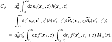 (18)with
  , where we introduced the window function f(x), which is nonzero inside the Faraday screen:
 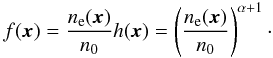 (19)
(19) is the zz-part of the (rescaled) magnetic autocorrelation tensor, which we try to measure.
3.5. Modelling the magnetic autocorrelation
Mzz(r) can be split up into a longitudinal part ML(r) and a corresponding perpendicular part MN(r), which depend only on the absolute value of r (see Subramanian 1999; or Enßlin & Vogt 2003).  (20)The rescaled magnetic autocorrelation function
  is given by
 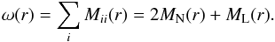 (21)The information of the data can be combined into a one-dimensional correlation function and therefore does not allow us to simultaneously determine two independent functions. Thus a relation between MN and ML is necessary. There are two suitable possibilities how to connect them.
-
a)
Full isotropy assumption, which additionally assumesisotropy at any location in Fourier space. This yields
 (22)
(22) -
b)
Considering the solenoidal character of the magnetic field by
 , which yields
  (23)
(23)
condition leads to Eq. (6) and is more physical, but also more complicated to handle. Both assumptions have been implemented in REALMAF. However, the most computationally efficient way is to use the full isotropy assumption and apply the divergence relation in Fourier space, which results in a simple multiplication factor, see Sect. 3.6.
Connecting of ML and MN allows us to parameterise Mzz(r) using  (24)where
  is further split into
  and
and  described by Eq. (20). Because of the linearity of the Fourier transformation, the linear coefficients si in real space also appear as linear coefficients in the analogous representation in Fourier space. Thus, although we are calculating the covariance matrix completely in real space, the power spectrum can be obtained directly:
 The basis functions together with the retrieved spectral amplitudes si can be translated into ω(r) (see Fig. 1a) and the corresponding ω(k) (see Fig. 1b). The used model functions for
  and
and  were chosen to transform into relatively well separated and well localised frequency bands wi(k) in Fourier space. Appendix A shows the used model functions and describes how they were derived.
3.6. The divergence relation in Fourier space
The zz-part of the magnetic autocorrelation tensor can be expressed in Fourier space analogously to Eq. (20)  (25)Applying gives then
  (26)see Enßlin & Vogt (2003). The
  from Eq. (25) is in general not the Fourier transformation of ML(r) used in Eq. (20). To create a connection to the real-space parameterisation Mzz(r), we multiply
  by 3/2, which is analogous to an addition of with
  . This makes Mzz(k) a spherically symmetric function, which forces that its Fourier back-transform Mzz(r) must be spherically symmetric as well. Then,
  (27)which is the full isotropy assumption defined in Eq. (22). Therefore, when assuming full isotropy, the divergence condition can be imposed on ω(k) to a good approximation via multiplying it with the factor 2/3. This was verified as well by numerical experiments2. Using the full isotropy assumption reduces the processing time by up to a factor 4 and allows a simpler spherically symmetric model for Mzz. In practice the power spectrum is multiplied with a factor 2/3 and the resulting magnetic field strength by
  .
.
Finally, the condition, which is used by Vogt & Enßlin (2005) as well, is not exact because of
 with the rescaleing function h defined in Sect. 3.4. If B varies on scales much smaller than the ones on which h varies, this assumption is sufficiently close to the condition ∇·B = 0. Another indication that the resulting errors are negligibl small is that a totally different assumption on the statistical distribution of the magnetic fields, like full isotropy, which violates by definition, produces only a shift by a factor of 1.5, as shown above.
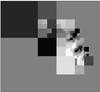 |
Fig. 2 Merged data map of Hydra A with 1000 pixels remaining. The RM values range between –1700 rad/m2 (dark) and 2800 rad/m2 (light). The map has a size of about 40 kpc. Each square represents one value used in the analysis. |
4. Application to the Hydra A data
4.1. The data
High-resolution polarisation measurements of the radio lobes of Hydra A at different wavelengths, with the VLA suitable for RM map making, were performed by Taylor & Perley (1993). High-fidelity RM maps were constructed from these using the PACERMAN code (Dolag et al. 2005; Vogt et al. 2005). PACERMAN uses error weighting and also non-local information to solve the nπ-ambiguity and therefore produces more reliable Faraday rotation maps than algorithms that do standard fitting of Eq. (2) pixel by pixel. The resulting RM map was tested by Vogt et al. (2005) for the presence of map-making artifacts. These artifacts can be statistically detected using the anti-correlation of inferred RM and position angle values imprinted by misfits, as first shown by Enßlin et al. (2003). The tests show that the current RM map of the south lobe of Hydra A is prone to nπ-ambiguities and other artifacts, even if generated with PACERMAN. However, the north lobe, which contains lower RM values and is therefore pointing towards us, is sufficiently clean. Therefore Vogt & Enßlin (2005) analysed only the north lobe of Hydra A, and our application of REALMAF is also restricted to this area.
The resolution of the RM map is too high to take every single pixel into account in our analysis. A computational bottleneck is the double integral in the calculation of the model covariance matrix followed by matrix multiplications described in Sect. 3.3. To reduce the amount of required computational resources, we merge areas in the map to bigger pixels by combining the rotation measure values, the errors, and the pixel position in an inverse noise-weighted fashion. The idea is to average the data in quadratic areas chosen so that they have roughly the same noise level. Therefore the outer regions with lower radio surface brightness and consequently larger RM errors are more heavily averaged. For details on the algorithm combining the pixels, the reader is referred to Vogt & Enßlin (2005).
These merged data points then form the data vector d used in Sect. 3.2. Figure 2 visualises the merged map by showing the averaged values in colour within the square areas from which they were averaged. The area outside the squares does not contain any used RM values. In Fig. 3 the radial profile of of RM2 is shown and is compared with the ensemble averaged ⟨ RM2 ⟩ predicted by the deduced magnetic spectrum and assumed radial profile of the electron and magnetic field energy densities. From this figure it can be seen that the largest separation between our pixels is rmax = 33 kpc, whereas the smallest rmin = 0.073 kpc. A first guess of the optimal spectral range can be obtained based on these maximal and minimal sizes of visible structures calculated using kmin = π/rmax and kmax = π/rmin The final result in Fig. 7 uses roughly these spectral boundaries.
Spatial averaging of RM data is not properly modelled in Eq. (18). In principle, it could be included into this formula and the generic inference formalism, owing to the linearity of averaging. However, we have to perform the double integral in Eq. (18) numerically for any pair of data pixels. Adding four more integration dimensions would exceed our computational possibilities.
We accept the spectral error resulting from the data averaging operation because pixels that resulted from averaging over large regions are automatically only contributing information about scales above their size. Any baseline formed by them with other pixels will be of the order of the pixel size or larger. The product of the RM values of a pair of pixels is compared with the expected data correlation over this baseline distance. Thus these pixels determine the inferred spectrum mostly on scales on which their internal RM substructure, which was averaged out, does not matter.
The silhouette of the radio lobe used to probe the Faraday screen breaks the translational invariance of our problem, in addition to the effect of the electron density profile. However, this does not impact directly our data covariance matrix C, because this only contains the expected (averaged over an ensemble of data realisations) correlation of individual pairs of positions in the RM map. The silhouette restricts the available positions and therefore the number of baselines, which means that on larger scales, we have less information. However, the Bayesian formalism is informed about this and just increases the uncertainty margins for poorly constrained data modes.
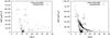 |
Fig. 3 Left: radial profile of the original rotation measure data and the merged values shown in Fig. 2. To facilitate reading of the plot, the 1000 merged data points are combined within (variably sized) radial bins. Right: comparison of the merged profile with the theoretical radial profile of the ensemble average resulting from the analysis. The retrieved profile was obtained from the trace of the covariance matrix described in Eq. (18) and implicitly emerges from the modelled magnetic power spectrum shown in Fig. 8 and the assumed geometrical profiles of magnetic energy and electron density. The former determines the amplitude of the theoretical profile, whereas the latter determines the detailed radial decline. This theoretical curve was not obtained by a fit of the radial profile, which is shown here for illustration only. Instead, our inference is based on examining the cross-correlation of all pairs of points, which contain much more information compared with the autocorrelation of individual points displayed here. We note that the variations seen in the data with respect to the theoretical mean curve are a natural consequence of the data being only a single realisation of a random process, whereas the theoretical curve represents the ensemble average of a large number of these realisations. |
We also require to specify the noise covariance matrix. Assuming the noise at different pixels to be uncorrelated, the noise matrix is diagonal. The diagonal elements can be approximated by the square of the RM-deviation of each pixel given by the error map produced by PACERMAN.
The used rotation measure map has a mean value of about 600 rad/m2. The galactic rotation measure at the position of Hydra A is about 1 percent of this and therefore negligible, see Johnston-Hollitt et al. (2004). Therefore we assume that the mean value is caused by cosmic variance which is in turn processing a too small sample of the cluster. This mean value is correctly interpreted by our method in that it adds power to the small k part of the magnetic power spectrum, compared with the case in which we subtract the mean value from the data d.
4.2. Window function
The window function f defined in Eq. (19) requires the electron density distribution ne(x). Hydra A is a cooling-core cluster. Therefore we assume a spherically symmetric double beta profile defined as ![Mathematical equation: \begin{equation} \label{eq:windowfunction} {n_{\rm e}(x)= \left[ n_{{\rm e}1}^2 \left(1+ \left( \frac{r}{r_{\rm c1}} \right)^2 \right)^{-3\beta} + n_{{\rm e}2}^2 \left( 1+\left( \frac{r}{r_{\rm c2}}\right)^2 \right)^{-3\beta} \right]^{1/2}}, \end{equation}](/articles/aa/full_html/2011/05/aa13918-09/aa13918-09-eq154.png) (28)with ne1 = 0.056 cm-3, ne2 = 0.0063 cm-3, rc1 = 33.3 kpc, rc2 = 169 kpc and β = 0.766, as fitted by Vogt & Enßlin (2005) using data from Mohr et al. (1999). Various works propose that the observed radio lobes of active galactic nuclei, like Hydra A, form cavities in the cluster atmosphere, see e.g. Böhringer et al. (1993), Enßlin (1999), McNamara et al. (2000), Fabian et al. (2000), and David et al. (2001). In these cavities the polarised radio light is produced, but ne(x) is presumably so low that no significant Faraday rotation is expected to occur there. The fact ne(x) = 0 for any x ∈ cavity can be taken into account by adjusting the integration boundaries in Eq. (18). In order to calculate the important lower integration boundary, where the Faraday active area starts, we need to know the geometry of the cavity. The cavity in our used map-section can be approximated by an ellipse with the projected distance 24.9 kpc from cluster centre, projected semimajor axis 20.5 kpc, and semiminor axis with 12.4 kpc, as Wise et al. (2007) propose. Additionally the Hydra A north lobe is tilted by an angle θ towards the observer. Depending on θ the innermost radius of the probed Faraday active area shifts, as can be seen in Fig. 4. There it becomes apparent that the sensitivity of our analysis starts at radii of about 20 to 30 kpc from the cluster centre depending on θ. θ is not well determined and its estimates range from about 30° (Taylor & Perley (1993), if the cavity effect is added) to more than 45° (Laing et al. 2008) to 60° (Wise et al. 2007).
(28)with ne1 = 0.056 cm-3, ne2 = 0.0063 cm-3, rc1 = 33.3 kpc, rc2 = 169 kpc and β = 0.766, as fitted by Vogt & Enßlin (2005) using data from Mohr et al. (1999). Various works propose that the observed radio lobes of active galactic nuclei, like Hydra A, form cavities in the cluster atmosphere, see e.g. Böhringer et al. (1993), Enßlin (1999), McNamara et al. (2000), Fabian et al. (2000), and David et al. (2001). In these cavities the polarised radio light is produced, but ne(x) is presumably so low that no significant Faraday rotation is expected to occur there. The fact ne(x) = 0 for any x ∈ cavity can be taken into account by adjusting the integration boundaries in Eq. (18). In order to calculate the important lower integration boundary, where the Faraday active area starts, we need to know the geometry of the cavity. The cavity in our used map-section can be approximated by an ellipse with the projected distance 24.9 kpc from cluster centre, projected semimajor axis 20.5 kpc, and semiminor axis with 12.4 kpc, as Wise et al. (2007) propose. Additionally the Hydra A north lobe is tilted by an angle θ towards the observer. Depending on θ the innermost radius of the probed Faraday active area shifts, as can be seen in Fig. 4. There it becomes apparent that the sensitivity of our analysis starts at radii of about 20 to 30 kpc from the cluster centre depending on θ. θ is not well determined and its estimates range from about 30° (Taylor & Perley (1993), if the cavity effect is added) to more than 45° (Laing et al. 2008) to 60° (Wise et al. 2007).
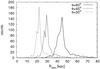 |
Fig. 4 Histogram of the minimal distance Rmin from the cluster centre for 800 data points depending on the assumed projection angle θ. Magnetic fields at r < Rmin are invisible to the method. |
4.3. Measuring the magnetic profile
The index α of the magnetic field can be retrieved from the data. In contrast to the power spectrum3, which is built dynamically by our algorithm, α has to be set up for every processing run. Maximising the posterior with respect to α provides indications on most probable configurations. One drawback is that α also depends on the low-frequency cut-off kmin (position of the top of the first spectral bin) chosen; meaning a two-dimensional problem needs to be optimised. The result we find is α = 1 with kmin = 0.42 kpc-1. Because this result only depends on the large scales, a rather low-resolution study with 300 data points was sufficient and permitted a fast investigation of the 2-d parameter space. Sampling of kmin for three different projection angles θ can be found in Fig. 5.
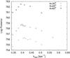 |
Fig. 5 Sampling of kmin for given α = 1. |
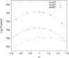 |
Fig. 6 Sampling of α for given kmin = 0.42 kpc-1. |
Cut-offs with k < 0.42 kpc-1 correspond to α > 1 and vice versa. Smaller θ implies a smaller physical distance between the data points, which results in a small shift of kmin. However, it is negligible and inside the statistical variance of about 0.05 kpc-1. Figure 6 shows a consistency check by sampling α for the given kmin = 0.42 kpc-1. The curvature in Fig. 6 gives roughly a 1-sigma variance for α of about Δα = ± 0.3, while assuming Gaussianity around the peak. When we also consider the impact of the variance of kmin, we find α = 1 ± 0.5.
Surprisingly the posterior maximum is rising for rising θ with no apparent limit. We suppose that this has nothing to do with the probability of the physical model and therefore θ cannot be restricted using the data of the Hydra A north lobe only. Indeed, θ is a parameter, that only affects the integration bounds of Eq. (18), whereas the power spectrum, the magnetic scaling α, and the cut-offs affect the integrand.
4.4. Power spectrum and magnetic characteristics
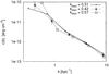 |
Fig. 7 Power spectrum with an optimal, a too small and a too large cut-off kmin. |
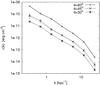 |
Fig. 8 Inferred power spectrum for three assumed projection angles and comparison with a Kolmogorov slope (dotted). Note that for k > 10 kpc-1 beam effects reduce the amount of power and are probably responsible for the steepening. |
The shape of the power spectrum depends on the spectral cut-offs kmin and kmax. We retrieved the most probable kmin to be 0.42 kpc-1 in Sect. 4.3. Obviously, the most probable configuration is a power law with no large-scale turnover visible within the probed spatial scales, as can be seen in Fig. 7. The decline for smaller kmin may be caused by the limited rotation measure map dimensions and the down-pull of thereby unconstrained amplitudes by Jeffreys prior. A larger kmin will remove necessary degrees of freedom of the model at the large scales, which forces the algorithm to deposit additional power at the neighbouring scale. The high-frequency cut-off is limited by the resolution of the map and instrumental beam. A beam with spatial scales of 0.32 kpc (FWHM) gives kmax = 10 kpc-1. Below, we increase the resolution by increasing the number of data points to 1000 and extend the spectrum to a maximal possible range. We made three processing runs with α = 1 and three possible projection angles, see Fig. 8 and Table 1. To investigate the dependence of the results on α we made two more runs with α = 0.5 and α = 1.5, see Table 2. Formulas for the calculation of the magnetic characteristics are described in Appendix B. The given statistical uncertainties refer to static α and θ. These errors are propagated from the error bars of the power spectrum.
Magnetic field characteristics for most probable α = 1.
Magnetic field characteristics for θ = 45° and maximal and minimal possible α.
The power law ranges from scales of 0.3 kpc (beam FWHM) to about 8 kpc. The fall-off in power at small scales is caused by instrumental beam effects. However, the larger scales are not greatly affected by the beam. To measure the spectral index we ignore the first spectral bin, which is possibly affected by map boundary limits as well as the last two beam affected bins. The dotted line in Fig. 8 represents a Kolmogorov slope of ϵ(k) ∝ k-1.67 compared with the plot using θ = 45°. We achieve a perfect fit for the central part of the retrieved power spectrum, which is also inside the larger statistical variance of the parts at smaller k. There is a noticeable dependence of the spectral index on α with minimal and maximal slopes of 1.5 and 2.1, which should be regarded as improbable worst cases. θ has a big impact on the resulting magnetic field strengths. Assuming a larger θ implies a shorter interaction path with the magnetic field and therefore greater necessary magnetic field strengths. The derived B0 in the cluster centre assumes that the magnetic profile given by Eq. (17) can be extrapolated with a constant α into the cluster centre. However, the sensitivity starts at regions from about 30 kpc from the cluster centre, see Fig. 4, and a flattening of the magnetic profile at smaller radii is well possible. B50 gives the directly probed magnetic field strengths at 50 kpc distance.
The impact of the instrumental beam on the calculated magnetic field strength is low. A continuation of the power law to the small scales would give an additional 0.2 μG at most.
5. Comparison with other methods
Recent results of Hydra A for θ = 45°.
The magnetic power spectrum of Hydra A was previously measured by Vogt & Enßlin (2005) and by Laing et al. (2008). Both find significantly lower central magnetic field strengths than we do. This is because of a much flatter magnetic field profile inferred characterised by a smaller index α. Moreover Vogt & Enßlin (2005) found a bump, a cut-off at spatial scales of about 2 kpc and more, but the spectral index for small scales is still similar to our current results. However, Laing finds a much flatter spectral index of about 0.8. Table 3 compares the results for a projection angle of θ = 45°.
To partly reconstruct the results of Vogt & Enßlin (2005), we applied the two simplifications they have used in the calculation of the covariance matrix in Eq. (18),
-
1.
extending the second lower integration bound to –∞;
-
2.
merging the two window functions f assuming the magnetic autocorrelation changes on much smaller scales than the window function.
Then we compared the results with the Fourier method of Vogt, but adding noise effects, the cavity structure, and a more advanced triangular parameterisation of the power spectrum, see Fig. 9. We reconstructed the spectral bump found by Vogt & Enßlin (2005) and found a perfect match between both methods. Figure 10 shows the difference to our method without these simplifications.
Consistent with Vogt & Enßlin (2005), the most likely α is shifted to much lower values if one adopts these simplifications, as can be seen in Fig. 11. However, instead of a falling plateau of the posterior between α = 0.1 and α = 0.8 and a cut-off for the unphysical range α < 0.1 we again find a Gaussian distribution, but with a maximum at 0.1. This very low α value indicates that the bump found by Vogt & Enßlin (2005) may be explained by a power leak on large scales produced by an implicit increase of the large-scale contribution of the window function.
One of the major simplifications used by Laing et al. (2008) is a linear and position-independent relation between the RM power spectrum and the magnetic autocorrelation4, which is only valid for a deep and statistically homogeneous Faraday screen. Both assumptions are not very well met for the Hydra A cluster. If we simulate a constant window function by setting α = −1 (for which the effective window function, as given by Eq. (19), becomes flat) and use symmetric integration bounds in Eq. (18) we get a spectral index of about 1.1. For α = 0.25 we get a central magnetic field strength of 12.9 μG, which is much closer to their results.
The remaining difference to the spectral index of 0.8 and field strength of 19 μG may be partly caused by the beam correction applied by Laing et al. (2008), which lifts the high-frequency part of the spectrum, which is possibly contaminated with noise residuals from the RM-map-making algorithms. An implementation of a beam correction as a convolution in real space is not feasible in REALMAF, because it would be computationally too expensive and an implementation in Fourier space is in general only possible with simplifying assumptions. However, the exact frequency-dependent instrumental beam is unknown anyway, and we believe its effect can be neglected at scales larger than the beam size.
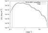 |
Fig. 9 Reconstruction of the results of the Fourier space method by Vogt & Enßlin (2005) by adding the removed simplifications for α = 0.5 and θ = 45°. This plot illustrates the continuous result taking the model for the power spectrum into account. |
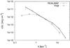 |
Fig. 10 Power spectrum using the REALMAF and the method by Vogt & Enßlin (2005) for α = 0.5 and θ = 45°. According to Fig. 9 the Fourier method is equivalent to explicitly adding simplifications to the real space method. |
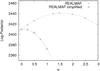 |
Fig. 11 Sampling of α with and without simplifications used in Vogt & Enßlin (2005) for θ = 45° and kmin = 0.3 kpc-1. |
6. Conclusions
6.1. Summary
We developed a new method to retrieve magnetic power spectra from Faraday rotation maps implemented in the REALMAF (REAL MAgnetic Fields) code, where we modelled the magnetic autocorrelation function in real space.
Furthermore we introduced and verified a way to take the solenoidal character of the magnetic fields into account by using a simple full spherical model for the magnetic autocorrelation and multiplying with a proportionality factor. In contrast to the method by Vogt & Enßlin (2005) with a model in Fourier space, this permits us to alleviate some previously required simplifications in the processing. However, we are able to reconstruct their results by synthetically adding their simplifications to our method.
When we apply REALMAF to the north lobe of the Hydra A galaxy cluster, we find a power law power spectrum in the spatial range of 0.3 kpc to 8 kpc, with no visible large-scale turnover within this range, as reported by Vogt & Enßlin (2005). The magnetic density profile, which we modelled with an index α applied to the electron density profile, seems to follow the electron density profile with α = 1 ± 0.5. The somewhat large uncertainty on α also affects the spectral index of the power law, which is then in the range of 1.5 to 2.1. The exact projection angle of the used radio lobe Hydra A north is not well restricted, but it only seriously affects the absolute value of the magnetic energy density in the cluster and not the spectral slope. Depending on the angle we obtain field strengths ranging from 20 μG up to 80 μG in the cluster centre. However, these are extrapolations, because the measurement is only sensitive at a distance of about 50 kpc from cluster centre, where we find fields between 10 μG and 30 μG. The extrapolation of the model into the centre may be questionable.
Theories describing the generation of magnetic fields by turbulence like Subramanian et al. (2006), Enßlin & Vogt (2006) and Schekochihin & Cowley (2006) forecast a large-scale turnover, which might be visible inside our spectral range. Compared with Vogt & Enßlin (2005) we found no large-scale turnover within the spectral range up to 8 kpc. A turnover at larger scales is, however, not excluded by our analysis.
6.2. Outlook
The REALMAF code will permit us to analyse the Faraday rotation data of other galaxy clusters. This will hopefully allow us to study magnetic field spectra over a large range of spatial scales and in a variety of cluster environments. A usable map of Hydra A south would further increase the probed range at large scales and a map with a higher resolution would increase the range at small scales. We published the REALMAF code for general scientific usage under an open source license5.
Upcoming telescopes such as EVLA, LOFAR, LWA, ASKAP, and SKA will certainly provide the necessary high-fidelity Faraday rotation data of many more galaxy clusters for further studies with REALMAF. This may help to figure out the origin of cluster magnetic fields and the role they play in the metabolism of the intra-cluster medium.
The algorithm described Sect. 3.3 may not converge and may fail in cases where the variance of the spectrum is too large, or, equivalently, the inverse problem is too degenerate. For the our data this limits the spectral resolution to a maximum of about 7 bins.
Actually this relation was discovered in numerical experiments first.
And the directly obtained central magnetic field strength B0.
Applied by Vogt & Enßlin (2003) as well.
Acknowledgments
Special thanks to Corina Vogt, who made her code used in Vogt & Enßlin (2005) available for insight, thanks to Daria Guidetti and Robert Laing for discussions and to an anonymous referee for constructive comments, and thanks to Henrik Junklewitz and Niels Oppermann for comments on the manuscript. This research was performed in the framework of the DFG Forschergruppe 1254 “Magnetisation of Interstellar and Intergalactic Media: The Prospects of Low-Frequency Radio Observations”.
References
- Battaglia, N., Pfrommer, C., Sievers, J. L., Bond, J. R., & Enßlin, T. A. 2009, MNRAS, 393, 1073 [NASA ADS] [CrossRef] [Google Scholar]
- Böhringer, H., Voges, W., Fabian, A. C., Edge, A. C., & Neumann, D. M. 1993, MNRAS, 264, L25 [NASA ADS] [CrossRef] [Google Scholar]
- Bonafede, A., Feretti, L., Murgia, M., et al. 2010a, A&A, 513, A30 [NASA ADS] [CrossRef] [EDP Sciences] [Google Scholar]
- Bonafede, A., Feretti, L., Murgia, M., et al. 2010b, [arXiv:1009.1233] [Google Scholar]
- Carilli, C. L., & Taylor, G. B. 2002, ARA&A, 40, 319 [NASA ADS] [CrossRef] [Google Scholar]
- Cho, J., & Ryu, D. 2009, ApJ, 705, L90 [NASA ADS] [CrossRef] [Google Scholar]
- Clarke, T. E., Kronberg, P. P., & Böhringer, H. 2001, ApJ, 547, L111 [NASA ADS] [CrossRef] [Google Scholar]
- David, L. P., Nulsen, P. E. J., McNamara, B. R., et al. 2001, ApJ, 557, 546 [NASA ADS] [CrossRef] [Google Scholar]
- de Vaucouleurs, G., de Vaucouleurs, A., Corwin, Jr., H. G., et al. 1991, Third Reference Catalogue of Bright Galaxies [Google Scholar]
- Dennison, B. 1979, AJ, 84, 725 [NASA ADS] [CrossRef] [Google Scholar]
- Dolag, K., Schindler, S., Govoni, F., & Feretti, L. 2001, A&A, 378, 777 [NASA ADS] [CrossRef] [EDP Sciences] [Google Scholar]
- Dolag, K., Bartelmann, M., & Lesch, H. 2002, A&A, 387, 383 [NASA ADS] [CrossRef] [EDP Sciences] [Google Scholar]
- Dolag, K., Vogt, C., & Enßlin, T. A. 2005, MNRAS, 358, 726 [NASA ADS] [CrossRef] [Google Scholar]
- Dreher, J. W., Carilli, C. L., & Perley, R. A. 1987, ApJ, 316, 611 [NASA ADS] [CrossRef] [Google Scholar]
- Eilek, J. A., & Owen, F. N. 2002, ApJ, 567, 202 [NASA ADS] [CrossRef] [Google Scholar]
- Enßlin, T. A. 1999, in Diffuse Thermal and Relativistic Plasma in Galaxy Clusters, ed. H. Boehringer, L. Feretti, & P. Schuecker, 275 [Google Scholar]
- Enßlin, T. A., & Vogt, C. 2003, A&A, 401, 835 [NASA ADS] [CrossRef] [EDP Sciences] [Google Scholar]
- Enßlin, T. A., & Vogt, C. 2006, A&A, 453, 447 [NASA ADS] [CrossRef] [EDP Sciences] [Google Scholar]
- Enßlin, T. A., Vogt, C., Clarke, T. E., & Taylor, G. B. 2003, ApJ, 597, 870 [NASA ADS] [CrossRef] [Google Scholar]
- Fabian, A. C., Sanders, J. S., Ettori, S., et al. 2000, MNRAS, 318, L65 [NASA ADS] [CrossRef] [Google Scholar]
- Feain, I. J., Ekers, R. D., Murphy, T., et al. 2009, ApJ, 707, 114 [NASA ADS] [CrossRef] [Google Scholar]
- Feretti, L., Dallacasa, D., Giovannini, G., & Tagliani, A. 1995, A&A, 302, 680 [NASA ADS] [Google Scholar]
- Feretti, L., Dallacasa, D., Govoni, F., et al. 1999a, A&A, 344, 472 [NASA ADS] [Google Scholar]
- Feretti, L., Perley, R., Giovannini, G., & Andernach, H. 1999b, A&A, 341, 29 [NASA ADS] [Google Scholar]
- Ge, J., & Owen, F. N. 1994, AJ, 108, 1523 [NASA ADS] [CrossRef] [Google Scholar]
- Goldshmidt, O., & Rephaeli, Y. 1993, ApJ, 411, 518 [NASA ADS] [CrossRef] [Google Scholar]
- Govoni, F., Murgia, M., Feretti, L., et al. 2006, A&A, 460, 425 [NASA ADS] [CrossRef] [EDP Sciences] [Google Scholar]
- Govoni, F., Dolag, K., Murgia, M., et al. 2010, A&A, 522, A105 [NASA ADS] [CrossRef] [EDP Sciences] [Google Scholar]
- Guidetti, D., Murgia, M., Govoni, F., et al. 2008, A&A, 483, 699 [NASA ADS] [CrossRef] [EDP Sciences] [Google Scholar]
- Hennessy, G. S., Owen, F. N., & Eilek, J. A. 1989, ApJ, 347, 144 [NASA ADS] [CrossRef] [Google Scholar]
- Johnson, R. A., Leahy, J. P., & Garrington, S. T. 1995, MNRAS, 273, 877 [NASA ADS] [Google Scholar]
- Johnston-Hollitt, M., Hollitt, C. P., & Ekers, R. D. 2004, in The Magnetized Interstellar Medium, ed. B. Uyaniker, W. Reich, & R. Wielebinski, 13 [Google Scholar]
- Kim, K., Kronberg, P. P., & Tribble, P. C. 1991, ApJ, 379, 80 [NASA ADS] [CrossRef] [Google Scholar]
- Laing, R. A. 1988, Nature, 331, 149 [NASA ADS] [CrossRef] [Google Scholar]
- Laing, R. A., Canvin, J. R., Cotton, W. D., & Bridle, A. H. 2006, MNRAS, 368, 48 [NASA ADS] [Google Scholar]
- Laing, R. A., Bridle, A. H., Parma, P., & Murgia, M. 2008, MNRAS, 391, 521 [NASA ADS] [CrossRef] [Google Scholar]
- Lawler, J. M., & Dennison, B. 1982, ApJ, 252, 81 [NASA ADS] [CrossRef] [Google Scholar]
- McNamara, B. R., Wise, M., Nulsen, P. E. J., et al. 2000, ApJ, 534, L135 [CrossRef] [Google Scholar]
- Mohr, J. J., Mathiesen, B., & Evrard, A. E. 1999, ApJ, 517, 627 [NASA ADS] [CrossRef] [Google Scholar]
- Murgia, M., Govoni, F., Feretti, L., et al. 2004, A&A, 424, 429 [NASA ADS] [CrossRef] [EDP Sciences] [Google Scholar]
- Schekochihin, A. A., & Cowley, S. C. 2006, Physics of Plasmas, 13, 056501 [NASA ADS] [CrossRef] [Google Scholar]
- Subramanian, K. 1999, Phys. Rev. Lett., 83, 2957 [NASA ADS] [CrossRef] [Google Scholar]
- Subramanian, K., Shukurov, A., & Haugen, N. E. L. 2006, MNRAS, 366, 1437 [NASA ADS] [CrossRef] [Google Scholar]
- Taylor, G. B., & Perley, R. A. 1993, ApJ, 416, 554 [NASA ADS] [CrossRef] [Google Scholar]
- Taylor, G. B., Perley, R. A., Inoue, M., et al. 1990, ApJ, 360, 41 [NASA ADS] [CrossRef] [Google Scholar]
- Taylor, G. B., Govoni, F., Allen, S. W., & Fabian, A. C. 2001, MNRAS, 326, 2 [NASA ADS] [CrossRef] [Google Scholar]
- Taylor, G. B., Fabian, A. C., & Allen, S. W. 2002, MNRAS, 334, 769 [NASA ADS] [CrossRef] [Google Scholar]
- Taylor, G. B., Fabian, A. C., Gentile, G., et al. 2007, MNRAS, 382, 67 [NASA ADS] [CrossRef] [Google Scholar]
- Vacca, V., Murgia, M., Govoni, F., et al. 2010, A&A, 514, A71 [NASA ADS] [CrossRef] [EDP Sciences] [Google Scholar]
- Vogt, C., & Enßlin, T. A. 2003, A&A, 412, 373 [NASA ADS] [CrossRef] [EDP Sciences] [Google Scholar]
- Vogt, C., & Enßlin, T. A. 2005, A&A, 434, 67 [NASA ADS] [CrossRef] [EDP Sciences] [Google Scholar]
- Vogt, C., Dolag, K., & Enßlin, T. A. 2005, MNRAS, 358, 732 [NASA ADS] [CrossRef] [Google Scholar]
- Waelkens, A. H., Schekochihin, A. A., & Enßlin, T. A. 2009, MNRAS, 398, 1970 [NASA ADS] [CrossRef] [Google Scholar]
- Wise, M. W., McNamara, B. R., Nulsen, P. E. J., Houck, J. C., & David, L. P. 2007, ApJ, 659, 1153 [NASA ADS] [CrossRef] [Google Scholar]
- Xu, Y., Kronberg, P. P., Habib, S., & Dufton, Q. W. 2006, ApJ, 637, 19 [NASA ADS] [CrossRef] [Google Scholar]
Appendix A: Model functions
Here we describe the construction of our spectral model functions. We start with an ansatz for ML(r) for the case  and use a Gaussian multiplied with a cosine. The corresponding MN(r) is obtained by Eq. (23). Thus we adopt
 ![Mathematical equation: \appendix \setcounter{section}{1} \begin{equation} \label{M(r)} \begin{aligned} M_\mathrm{L}^{(i)}(r) =& \frac{1}{\sqrt{2\pi}}b_i^3\exp[-\frac{1}{2}\frac{r^2}{a_i^2}]\cos[b_ir]\,,\,\textrm{and}\\ M_\mathrm{N}^{(i)}(r) =& \frac{b_i^3}{2a_i^2 \sqrt{2\pi}}\exp[{-\frac{r^2}{2a_i^2}}]((2a_i^2-r^2)\cos{[b_i r]}\\ &+ a_i^2 b_i r \sin{[b_i r]}). \end{aligned} \end{equation}](/articles/aa/full_html/2011/05/aa13918-09/aa13918-09-eq201.png) (A.1)These functions are Fourier transformed analytically using
(A.1)These functions are Fourier transformed analytically using
![Mathematical equation: \appendix \setcounter{section}{1} $$ M(k)=4\pi\int_0^\infty r^2 M(r)\frac{\sin{[k r]}}{k r}{\rm d}r, $$](/articles/aa/full_html/2011/05/aa13918-09/aa13918-09-eq202.png) see Enßlin & Vogt (2003). We bind the free parameter ai as
see Enßlin & Vogt (2003). We bind the free parameter ai as
 because in this case
 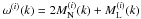 is fully positive and concentrated around a maximum at k = 3 bi. This allows us to put the power spectrum together by relatively well separated and located frequency bands, as Fig. A.2 illustrates. Figure A.1 shows the model functions in position space. Especially MN(r) has a strong negative part, because any closed field line has to come somewhere back through the plane perpendicular to it.
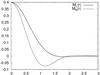 |
Fig. A.1 model functions |
If we assume full isotropy, Mzz(r) becomes spherically symmetric. In this case a suitable model function can be obtained by Eq. (A.1): 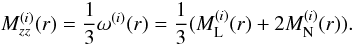 (A.2)This implicitly assumes MN(r) = ML(r). Thus we get
-
a)
using
in position space: ![Mathematical equation: \appendix \setcounter{section}{1} \begin{equation} \begin{aligned} M_\mathrm{L}^{(i)}(r)=&\frac{b_i^3}{\sqrt{2\pi}}\exp\Bigg[-\frac{8}{9} b_i^2 r^2\Bigg] \cos[b_i r]\\ M_\mathrm{N}^{(i)}(r)=& \frac{b_i^3}{18\sqrt{2\pi}}\exp\Bigg[-\frac{8}{9}b_i^2r^2\Bigg](2(9-8b_i^2r^2)\cos[b_ir]\\ &- 9b_ir\sin[b_ir]), \end{aligned} \end{equation}](/articles/aa/full_html/2011/05/aa13918-09/aa13918-09-eq212.png) (A.3)in Fourier space:
(A.3)in Fourier space: ![Mathematical equation: \appendix \setcounter{section}{1} \begin{equation} \begin{aligned} M_\mathrm{L}^{(i)}(k)=&\frac{27}{64}\pi\left(\frac{k-b_i}{k}\exp\Bigg[-\frac{9(b_i-k)^2}{32b_i^2}\Bigg]\right.\\ &+\left.\frac{k+b_i}{k}\exp\Bigg[-\frac{9(b_i+k)^2}{32b_i^2}\Bigg]\right)\\ M_\mathrm{N}^{(i)}(k)=&\frac{27}{128}\pi\left(\Bigg(\frac{9(b_i-k)^2}{16b_i^2}-1\Bigg)\exp\Bigg[-\frac{9(b_i-k)^2}{32b^2}\Bigg]\right.\\ &+\left. \Bigg(\frac{9(b_i+k)^2}{16b_i^2}-1\Bigg)\exp\Bigg[-\frac{9(b_i+k)^2}{32b_i^2}\Bigg]\right), \end{aligned} \end{equation}](/articles/aa/full_html/2011/05/aa13918-09/aa13918-09-eq213.png) (A.4)and
(A.4)and -
b)
using full isotropy in position space:
![Mathematical equation: \appendix \setcounter{section}{1} \begin{equation} \begin{aligned} M_{zz}^{(i)}(r)=&\frac{b_i^3}{27\sqrt{2\pi}}\exp\Bigg[-\frac{8}{9}b_i^2r^2\Bigg]\\ & \times\left((27-16b_i^2r^2)\cos[b_ir]-9b_ir\sin[b_ir]\right), \end{aligned} \end{equation}](/articles/aa/full_html/2011/05/aa13918-09/aa13918-09-eq214.png) (A.5)in Fourier space:
(A.5)in Fourier space: 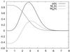
Fig. A.2 Model functions
 ,
,  and ω(i)(k) in Fourier space with
  and bi = 1.
![Mathematical equation: \appendix \setcounter{section}{1} \begin{equation} \begin{aligned} M_{zz}^{(i)}(k)=&\frac{27}{1024b_i^2k}\pi\exp\Bigg[-\frac{9(b_i+k)^2}{32b_i^2}\Bigg]\\ &\times\left(16b_i^3+9b_i^2k+18b_ik^2+9k^2+9k^3\right.\\ &+ \left.\exp\Bigg[\frac{9k}{8b_i}\Bigg]\Bigg(-16b_i^3+9b_i^2k-18b_ik^2+9k^3\Bigg)\right). \end{aligned} \end{equation}](/articles/aa/full_html/2011/05/aa13918-09/aa13918-09-eq218.png) (A.6)
(A.6)
Appendix B: Calculation of magnetic the field characteristics
Here we provide the used formulae for the magnetic field characteristics.
-
a)
Magnetic field strength The magnetic energy density can be calculated by integrating over the power spectrum or analogously taking the autocorrelation function in real space at the origin ω(0). The magnetic field strength in the centre of the cluster, where f = 1 and therefore
 , is then
  (B.1)
(B.1) -
b)
Magnetic autocorrelation length
 (B.2)
(B.2) -
c)
1-dimensional power spectrum Transformation from the three-dimensional power spectrum ω(k) to the one-dimensional ϵ(k) is done using (Enßlin & Vogt 2003)
 (B.3)
(B.3) -
d)
Spectral index using a Bayesian approach The spectral index can be calculated from the slope of the power spectrum in logarithmic scale. The fitting formula is:
 The variance from the above power law is then defined as:
  The allowed statistical deviations of s are imprinted in a covariance matrix Dij = ⟨ δsi δsj ⟩ , which is automatically obtained from the inverse of the Hessian matrix calculated with the maximum a posteriori approach as described in Sect. 3.3. The probabilities of the spectral amplitudes s of the power spectrum can be approximated as a Gaussian, where we can neglect the normalisation factor, because it is independent of q and r:
  Only a part of the power spectrum is used to fit the power law. Dij is then the projection (cut) of the full inverse Hessian matrix
  obtained from Eq. (16)
  with the projection operator ψ = { 0,...,1,...1,...,0 } selecting the used spectral bins for the fit. Using the Bayesian theorem from Eq. (13):
  where we already applied a uniform prior distribution P(r,q) = const. P(q,r | δs) has to be maximised to achieve the desired slope r within a maximum-a-posteriori approach. To numerically find the optimum, the gradients and the 2 × 2 Hessian matrix are necessary:
 ![Mathematical equation: \appendix \setcounter{section}{2} \begin{eqnarray*} \frac{\partial \ln P}{\partial r} &=& -q\ln[k_i]k_i^{-r}D_{ij}^{-1}(s_j-qk_j^{-r})\\ \frac{\partial \ln P}{\partial q} &=& k_i^{-r}H_{ij}^{-1}(s_j-qk_j^{-r})\\ \frac{\partial^2 \ln P}{\partial q^2} &=& -k_i^{-r}D_{ij}^{-1}k_j^{-r}\\ \frac{\partial^2 \ln P}{\partial r^2} &=& q(q\ln[k_i]k_i^{-r}D_{ij}^{-1}\ln[k_j]k_j^{-r}\\ &&-(\ln[k_i])^2k_i^{-r}D_{ij}^{-1}(s_j-qk_j^{-q}))\\ \frac{\partial^2 \ln P}{\partial q \partial r} &=& 2q\ln[k_i]k_i^{-r}D_{ij}^{-1}k_j^{-r}-\ln[k_i]k_i^{-r}D_{ij}^{-1}s_j. \end{eqnarray*}](/articles/aa/full_html/2011/05/aa13918-09/aa13918-09-eq241.png) An expression for the second unknown q can be found analytically. If the initial value of r is given, the corresponding initial value q can be calculated easily. This is necessary because the first guess must be close to the maximum to attain convergence.
An expression for the second unknown q can be found analytically. If the initial value of r is given, the corresponding initial value q can be calculated easily. This is necessary because the first guess must be close to the maximum to attain convergence. 
All Tables
All Figures
|
Fig. 1 Left: the magnetic autocorrelation ω(r) in position space for a typical magnetic power spectrum reconstruction for the cool core in the Hydra A cluster using seven spectral bins. The negative part of ω(r) is dotted. Right: the counterpart in Fourier space ω(k). The parameterisation can adopt any shape permitted by the seven basis functions seen as wiggles in the power spectrum. The parameters θ = 45° and α = 1 were assumed, with θ described in Sect. 4.2 and α introduced in Eq. (17). |
| In the text | |
|
Fig. 2 Merged data map of Hydra A with 1000 pixels remaining. The RM values range between –1700 rad/m2 (dark) and 2800 rad/m2 (light). The map has a size of about 40 kpc. Each square represents one value used in the analysis. |
| In the text | |
|
Fig. 3 Left: radial profile of the original rotation measure data and the merged values shown in Fig. 2. To facilitate reading of the plot, the 1000 merged data points are combined within (variably sized) radial bins. Right: comparison of the merged profile with the theoretical radial profile of the ensemble average resulting from the analysis. The retrieved profile was obtained from the trace of the covariance matrix described in Eq. (18) and implicitly emerges from the modelled magnetic power spectrum shown in Fig. 8 and the assumed geometrical profiles of magnetic energy and electron density. The former determines the amplitude of the theoretical profile, whereas the latter determines the detailed radial decline. This theoretical curve was not obtained by a fit of the radial profile, which is shown here for illustration only. Instead, our inference is based on examining the cross-correlation of all pairs of points, which contain much more information compared with the autocorrelation of individual points displayed here. We note that the variations seen in the data with respect to the theoretical mean curve are a natural consequence of the data being only a single realisation of a random process, whereas the theoretical curve represents the ensemble average of a large number of these realisations. |
| In the text | |
|
Fig. 4 Histogram of the minimal distance Rmin from the cluster centre for 800 data points depending on the assumed projection angle θ. Magnetic fields at r < Rmin are invisible to the method. |
| In the text | |
|
Fig. 5 Sampling of kmin for given α = 1. |
| In the text | |
|
Fig. 6 Sampling of α for given kmin = 0.42 kpc-1. |
| In the text | |
|
Fig. 7 Power spectrum with an optimal, a too small and a too large cut-off kmin. |
| In the text | |
|
Fig. 8 Inferred power spectrum for three assumed projection angles and comparison with a Kolmogorov slope (dotted). Note that for k > 10 kpc-1 beam effects reduce the amount of power and are probably responsible for the steepening. |
| In the text | |
|
Fig. 9 Reconstruction of the results of the Fourier space method by Vogt & Enßlin (2005) by adding the removed simplifications for α = 0.5 and θ = 45°. This plot illustrates the continuous result taking the model for the power spectrum into account. |
| In the text | |
|
Fig. 10 Power spectrum using the REALMAF and the method by Vogt & Enßlin (2005) for α = 0.5 and θ = 45°. According to Fig. 9 the Fourier method is equivalent to explicitly adding simplifications to the real space method. |
| In the text | |
|
Fig. 11 Sampling of α with and without simplifications used in Vogt & Enßlin (2005) for θ = 45° and kmin = 0.3 kpc-1. |
| In the text | |
|
Fig. A.1 model functions |
| In the text | |
|
Fig. A.2 Model functions |
| In the text | |
Current usage metrics show cumulative count of Article Views (full-text article views including HTML views, PDF and ePub downloads, according to the available data) and Abstracts Views on Vision4Press platform.
Data correspond to usage on the plateform after 2015. The current usage metrics is available 48-96 hours after online publication and is updated daily on week days.
Initial download of the metrics may take a while.