| Issue |
A&A
Volume 528, April 2011
|
|
|---|---|---|
| Article Number | A128 | |
| Number of page(s) | 6 | |
| Section | Extragalactic astronomy | |
| DOI | https://doi.org/10.1051/0004-6361/201016353 | |
| Published online | 14 March 2011 | |
Kinematics and stellar population of NGC 4486A
1
Université de Lyon, Université Lyon 1, 69622 Villeurbanne, France ;
CRAL, Observatoire de Lyon, CNRS UMR 5574, 69561 Saint-Genis Laval France
e-mail: This email address is being protected from spambots. You need JavaScript enabled to view it.
2
Institut für Astronomie, Universität Wien, Türkenschanzstraße 17, 1180 Wien, Austria
e-mail: This email address is being protected from spambots. You need JavaScript enabled to view it.
3
Instituto de Astrofísica de Canarias, La Laguna, 38200 Tenerife ;
Departamento de Astrofísica, Universidad de La Laguna, 38205 La Laguna, Tenerife, Spain
e-mail: This email address is being protected from spambots. You need JavaScript enabled to view it.
4
Dept. of Physics & Astronomy, Ghent University, Krijgslaan 281, S9, 9000 Ghent, Belgium
e-mail: This email address is being protected from spambots. You need JavaScript enabled to view it.
Received: 17 December 2010
Accepted: 2 February 2011
Abstract
Context. NGC 4486A is a low-luminosity elliptical galaxy harbouring an edge-on nuclear disk of stars and dust. It is known to host a super-massive black hole.
Aims. We study its large-scale kinematics and stellar population along the major axis to investigate the link between the nuclear and global properties.
Methods. We use long-slit medium-resolution optical spectra that we fit against stellar population models.
Results. The SSP-equivalent age is about 12 Gyr old throughout the body of the galaxy, and its metallicity decreases from [Fe/H] = 0.18 near the centre to sub-solar values in the outskirts. The metallicity gradient is −0.24 dex per decade of radius within the effective isophote. The velocity dispersion is 132 ± 3 km s-1 at 1.3″ from the centre and decreases outwards. The rotation velocity reaches a maximum  km s-1 at a radius 1.3 < rmax < 2″.
Conclusions. NGC 4486A appears to be a typical low-luminosity elliptical galaxy. There is no signature in the stellar population of the possible ancient accretion/merging event that produced the disk.
Key words: galaxies: individual: NGC 4486A / galaxies: elliptical and lenticular, cD / galaxies: kinematics and dynamics / galaxies: stellar content
© ESO, 2011
1. Introduction
NGC 4486A is a low-luminosity (MB = −17.77 mag) E2 galaxy belonging to the Virgo cluster. Its catalogue properties are summarized in Table 1. It is one of the four galaxies projected within a few arcmin of the central cD, M 87 (Prugniel et al. 1987). It habours a spectacular nuclear disk of stars and dust (Kormendy et al. 2005). This almost edge-on disk, detected up to a radius of 250–350 pc (3–4″, approximately half the effective radius, reff), is marginally bluer than the surrounding population, suggesting that it is at least 2 Gyr younger. It is aligned along the major axis of the galaxy. This disk is believed to have been formed from accreted gas that funneled down to the central region.
Although it is a bright galaxy, it is not often observed because of a foreground bright star located 2.5″ away from the nucleus (de Vaucouleurs & de Vaucouleurs 1964; de Vaucouleurs 1959). However, this particular circumstance makes this object a first choice target for adaptive optics observations. Kormendy et al. (2005) used the adaptive optics system of the CFH telescope to reach a spatial resolution of 0.07″ (FWHM) after a Lucy deconvolution. Nowak et al. (2007) used the near-infrared integral field spectrograph SINFONI to study the central kinematics. Using the Schwarzschild orbit superposition method to fit the two-dimensional information, they found a central super-massive black hole of mass M• = 1.25 × 10⁷ M⊙ and rejected any model without a black hole at the 4.5σ confidence level.
In this paper, we study the internal kinematics and the stellar population of this galaxy to investigate if its nuclear particularity is related to its global properties.
The paper is organized as follows: in Sect. 2 we present the observations and the data reduction, in Sect. 3 the analysis, and in Sect. 4 we discuss the results and conclude.
Characteristics of NGC 4486A.
Setup and journal of the observations.
2. Observations and data reduction
In the frame of another project (Koleva et al. 2011), we discovered observations of NGC 4486A in the Gemini Science Archive. They were taken with the GMOS spectrograph attached to the 8.1 m Gemini-South telescope in long-slit mode. The setup and journal of these observations are reported in Table 2. Two slightly different grating orientations were used to patch the holes in the wavelength coverage, which are caused by the separation between the three CCD detectors.
The observer probably ignored the presence of the star and inadvertently centred the slit on it, unfortunately missing the centre of the galaxy by about 1″ (Fig. 1). Nevertheless, these spectra provide a chance to probe the stellar population and the kinematics of this object.
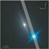 |
Fig. 1 Central field of NGC 4486A. The location of the slit is superimposed on the composite image from Kormendy et al. (2005, their Fig. 4). The size is 8″ across. |
The data reduction was made using the GMOS pipeline in the IRAF environment exactly as described in Koleva et al. (2011). The instrumental broadening, or line-spread function (LSF), was found to be acceptably modelled with a Gaussian with standard deviation σins = 61 km s-1. Some pixels within r = 0.6″ from the peak of light are saturated. The seeing measured on images taken during the same observing blocks is for the two nights 0.9 and 1.6″ FWHM with a typical error of ± 0.06″.
The radial position, r, of a spectrum with respect to the galaxy’s kinematical centre is related to the position along the slit with respect to the peak of light, x, as: r2 = (x + 2.15 ± 0.07)2 + (1.28 ± 0.07)2″2.
In order to measure the distance of the galaxy nucleus orthogonal to the slit, an ACS image of NGC 4486A obtained in the F850LP filter was extracted from the Hubble Legacy Archive. The distance between the star and the nucleus was determined to be 2.51 ± 0.05″ from measuring the position of the respective peaks of intensity. According to this measurement, the light peak of the galaxy in the slit should be at 2.36″ from the star. Fitting two Gaussians to the light distribution of the galaxy nucleus and the star in the GMOS acquisition image, which has been taken before the spectra, we measure a corresponding separation of 2.35 ± 0.08″. Using the light distribution of the spectrum along the slit, and fitting two Gaussians to the light peaks, we measure a separation of 2.45 ± 0.1.
Nowak et al. (2007) did not report any displacement of the kinematical centre, and therefore, we will not consider the small discrepancy between our photometric and kinematical determinations (one pixel, or one fifth of the FWHM seeing) as significant; it may result from the dust extinction. We adopt the kinematical centre as a reference.
3. Data analysis
The analysis was performed with the full-spectrum fitting package ULySS1 (Koleva et al. 2009).
The present difficulty of contamination by a foreground or background object was already met on other occasions. In Bouchard et al. (2010) and Makarova et al. (2010), the interloper was separately modelled and then subtracted before studying the target. In the present case, the contamination reaches 99% and extends over a large range of the object. We therefore tried to optimise the decomposition.
The ULySS package allows one to fit a spectrum against a constrained linear combination of non-linear models. In the present case we are considering two components that represent the star and the galaxy respectively. For the “star” component we could have attempted to use a spectrum extracted in the region where the galaxy spectrum is quasi-negligible. But we found a simpler and more robust way to model the stellar spectrum with ULySS, as in Wu et al. (2011). In this paper, stellar spectra are fitted against empirical models consisting of interpolated ELODIE spectra, and the authors show that this method reproduces accurately any observation and restores reliable atmospheric parameters.
The adopted model is therefore ![Mathematical equation: \begin{eqnarray} {\rm Obs}(\lambda, x) &=& P_n(\lambda) \times {\rm LSF}~\otimes \Big ( (1-f) \times S(T_{\rm eff}, g, \mathrm{[Fe/H]}_s, \lambda)\nonumber\\ \label{eqn:main} &&\quad+f \times G(cz, \sigma, h_3, h_4, {\rm Age}, \mathrm{[Fe/H]}_g, x, \lambda)\Big), \end{eqnarray}](/articles/aa/full_html/2011/04/aa16353-10/aa16353-10-eq35.png) (1)where Obs(λ,x) is the observed long-slit spectrum, function of the wavelength, λ, and position along the slit, x. S is the spectrum representing the foreground star, function of the atmospheric parameters (temperature, surface gravity and metallicity), and G is a synthetic stellar population, function of the radial velocity, velocity dispersion, h3 and h4 coefficients of the Gauss-Hermite expansion, age and metallicity for the position x along the slit. f is the relative light fraction of G, LSF is the line-spread function, and Pn is a multiplicative polynomial of degree n.
(1)where Obs(λ,x) is the observed long-slit spectrum, function of the wavelength, λ, and position along the slit, x. S is the spectrum representing the foreground star, function of the atmospheric parameters (temperature, surface gravity and metallicity), and G is a synthetic stellar population, function of the radial velocity, velocity dispersion, h3 and h4 coefficients of the Gauss-Hermite expansion, age and metallicity for the position x along the slit. f is the relative light fraction of G, LSF is the line-spread function, and Pn is a multiplicative polynomial of degree n.
The stellar model, S, is an interpolated empirical spectrum computed using the ELODIE library (Prugniel et al. 2007; Prugniel & Soubiran 2001). The population model, G, is computed with PEGASE.HR (Le Borgne et al. 2004) and is also based on the ELODIE library. We are using single stellar populations (SSPs) with a Salpeter (1955) IMF. An SSP supposes that all the stars are coeval and have the same metallicity. Because the two components S and G are based on the same spectral library, they share the same LSF (resolution R ≈ 10 000), and therefore the LSF can be factorized. The multiplicative polynomial, Pn, is modelling the shape of the spectrum and makes the flux calibration unnecessary. It was shown that even with flux-calibrated spectra, this polynomial is an advantage to match the inaccuracies of this calibration. We used a degree n = 40, determined as described in Koleva et al. (2009) which was also adopted in Koleva et al. (2011).
Because the stellar model does not depend on the position along the slit, it appears preferable to determine its parameters and to freeze them when analysing the galaxy. Therefore, the free parameters for the galactic fit are cz, σ, Age, [Fe/H ] g, f and the coefficients of Pn. There is only one more parameter than for a SSP fit. We discuss below the adjustment of the stellar model and then the fit of the galaxy.
3.1. Fit of the stellar spectrum
To determine the best ELODIE model to represent the foreground star, we first ran the analysis with the model of Eq. (1), leaving the stellar and galactic parameters free (as well as Pn). The retrieved parameters were very stable (i.e. independent of the position in the central two arcsec). Excluding the central spectra, because some pixels are saturated, we adopted the following solution: Teff = 6335 ± 5 K, log (g, cm s-2) = 4.14 ± 0.03 and [Fe/H ] = −0.33 ± 0.02. The quoted uncertainties reflect the dispersion of the values for the different extracted spectra (the physical uncertainties are larger, see Wu et al. 2011).
3.2. Kinematics and population of NGC 4486A
In order to check if this decomposition can bias the results, we applied the same analysis on another galaxy of the same observing run, which was un-affected by a star. We used NGC 4434 because it has approximately the same diameter, velocity dispersion, age, and metallicity as our present target. We found that the contribution of the stellar spectrum amounts to approximately 2%, which means that the flux contribution is comparable to the rms noise (the spectra were rebinned to reach S/N = 40). Because this contribution is constrained to be positive, we expected this component to be often inactive. Surprisingly, it is the case for only 3% of the individual spectra, independently of the radius of these extractions. These fake detections of the stellar component have no effect on the determination of the kinematics or of the age, but a small bias of 0.03 dex on the metallicity. This bias is acceptable for the present purpose.
We repeated the analysis of NGC 4486A using the atmospheric parameters determined in Sect. 3.1. The profiles obtained with the two setups are perfectly coincident, and the kinematics on the two sides of the galaxies fold adequately. The age is constant at 12 Gyr. The central metallicity is nearly solar, [Fe/H ] = 0.05 ± 0.02 dex, but the profile is asymmetric, declining to − 0.65 on the north side and to − 1 dex on the south at a radius of 10″. The light of the star exceeds the one from the galaxy by two orders of magnitude at the location of the star (the galactic spectrum is negligible at this place). The contamination then decreases, but remains at a level higher than 15% over the whole radial range.
This asymmetry of the metallicity is probably not physical, because the galaxy appears regular in other respects and this asymmetry is not observed in other galaxies. Therefore, we carefully examinated the fits and did additional tests. We separately analysed the blue and the red halves of the spectra and found consistent results (though naturally more noisy; the blue half was below 5000 Å, and the red above 4800 Å). When selecting the red region from 4900 Å (excluding Hβ), we obtained a marginal reduction of the asymmetry. We also tested with no more success, if allowing for a differential extinction between the star and the galaxy would reduce the effect and improve the fit.
The close examination of the fits revealed the probable presence of additional continuum light, in particular on the south side of the galaxy, which is more affected by the star. This pushes the solution to a lower metallicity and degrades the quality of the fit.
We then compared the light profiles along the slit for our target and for a template star observed with the same setup, and found that the contamination is actually higher than the one inferred from the spectroscopic decomposition. This provides additional evidence for pollution by diffuse light, which was not (or not perfectly) dispersed. The scattered light represents 1.5% of the incident light. Unfortunately, we did not have adequate observations to check if the PSF before the slit has indeed lower wings (the acquisition images are saturated).
Based on this suspicion of diffuse light, we fitted models with an additional free additive term. However, such a component is naturally degenerate with the metallicity, and the fit became unstable. It returned on average higher and super-solar [Fe/H ] g (as expected). We therefore added constraints.
We modified the model of Eq. (1) by replacing the stellar component, S, by a combination (1 − a) × S + a × C, where C is a constant spectrum representing the undispersed light and a the corresponding fraction. We adjusted a as the function of the distance to the star along the slit to match the retrieved spectroscopic contamination, f, with the photometric contamination obtained comparing our observation with one of a template star. We tried if using a different spectral energy distribution in place of the constant C affected the result and the quality of the fit. We considered either the same distribution as the star (using a smooth spectrum of it) or a spectrum biased to the blue (because the undispersed light may contaminate more the blue part of the spectrum). But we found no significant difference between these choices and adopted the additive constant. Because the age was apparently homogeneous, we fixed it to 12 Gyr to reduce the degree of freedom.
The final profiles of the kinematics and of the stellar population are presented in Fig. 2. We rejected the points in the range −1.3 < x < 1.9″ (1.5 < r < 4.2″ on the southern side), where the contamination from the foreground star exceeds the galactic light by more than a factor 2. An example of the decomposition is shown in Fig. 3 for the spectrum at the location x = 3,r = 5.6″, where the two contributions are comparable. The residuals are consistent with the noise computed from the photon statistics.
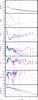 |
Fig. 2 Radial profiles of NGC 4486A derived from SSP fits. The spectra are radially binned for a compromise between S/N and spatial resolution (they have at minimum S/N = 40). The profiles are folded around the position of the kinematical centre. The red points are for the positive radii (South side) and blue for negative; the tones separate the two setups (the darker colours are for the first setup). The abscissa is the position along the slit (a = x − 2.15). The vertical blue dashed line marks the effective isophote. From top to bottom the panels are: (1) the logarithm of the relative total flux; (2) the logarithm of 1/f; (3 to 7) the internal kinematics and the SSP-equivalent metallicity. The velocity and h3 of the north side (blue points) are symmetrized. The points with f < 0.5 were excluded. |
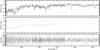 |
Fig. 3 Fit of a spectrum of NGC 4486A. The top panel shows the observed (in black) and fitted (blue) spectra. The red points mark the excluded regions (because of strong telluric absorption) and the rejected pixels (kappa-sigma clipping). The two gaps between the detectors are visible near 4800 and 5750 Å. The middle panel shows the two components of the model separately, the galactic population in black, and the star in orange. The bottom panel presents the residuals (observation-model). The green lines are the 1-σ errors. |
The kinematical, and now the metallicity, profiles are symmetric. The systemic velocity is 757 ± 6 km s-1. The peak of rotation velocity, Vmax = 107 ± 3, is reached at 2″ along the major axis (i.e. at a galactocentric distance of r = 2.4″). The velocity dispersion in our most central location, at 1.3″ along the minor axis, is σ0 = 132 ± 3 km s-1. Assuming a Gaussian line-of-sight velocity distribution (LOSVD), the peak rotation velocity is 96 km s-1 and the velocity dispersion σ0 = 139 ± 3 km s-1. The difference is due to the h3 and h4 moments. The h3 profile reveals a strong asymmetry of the LOSVD strongly correlated with the peak of rotation. After the peak, the rotation velocity and the velocity dispersion linearly decrease until 20″. The rotation decreases to 35 km s-1. The metallicity decreases linearly with radius from the central [Fe/H] = 0.18 dex to −1.3 dex at 20″.
Our analysis actually extends further than the 20″ limit of Fig. 2 (2.3 aeff), but owing to the lower S/N and strong contamination we have less confidence in these results. The radial velocity and metallicity appear well fitted, as the regularity and symmetry of the profiles show, but σ and the higher moments cannot be reliably determined. There is a hint that the rotation velocity continues to decrease and reaches 0 at 25–30″, but no indication that the outskirts would rotate in the opposite direction. This halo may be non-rotating. The metallicity continues to decrease to − 2 dex at 30″, and stays constant afterwards. However, the metallicity is the parameter that is the most affected by the contamination, and we will not interpret these external points.
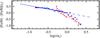 |
Fig. 4 Fit of the metallicity gradient. The colours are as in Fig. 2. The abscissa is the distance to the galaxy centre, divided by the effective semi-major axis. The straight line is the solution of the power-law fit, and its continuous region marks the used radial range. |
We fitted the metallicity gradients, ∇ [Fe/H ] = Δ [Fe/H ] /Δlog (r), using the points between the innermost location (r = 1.3″, greater than the seeing disk) and the effective isophote. The fit is shown in Fig. 4 and the value in Table 1. Clearly the adopted power-law model is not well suited (as in some other cases, see Koleva et al. 2011), but this fit allows us to compare this object with other galaxies. The flattening of the profiles in the most central region may be caused by the fact that the observation is made parallel to the major axis. The steepening after one reff, though consistent between the two sides and between the two setups, should be regarded with some caution, because the metallicity is the most sensitive parameter with respect to the pollution by diffuse light.
4. Discussion and conclusion
4.1. Revision of the catalogue properties
Because of the foreground star, the radial velocity and the velocity dispersion reported in the databases (HyperLeda and NED) are wrong. The velocity cz = 150 km s-1 and the dispersion σ0 = 41 ± 5 km s-1 obtained by the ENEAR project (Wegner et al. 2003) correspond to the stellar spectrum. The other earlier measurements are affected by the same problem.
4.2. Comparison with Nowak et al.
Nowak et al. (2007) find a kinematically cold component in the centre, with a velocity dispersion dropping to about σ0 = 110 km s-1. This structure coincides with the disk, and one arcsec above it, the velocity dispersion is in the range 130 to 140 km s-1. This is fully consistent with our value at the same location. The same method, using the near-infrared CO band heads, was used by Nowak et al. (2008) to study NGC 1316, which was also studied by us in the optical domain (Koleva et al. 2011). Our value of the velocity dispersion was significantly higher than the one of Nowak et al. (2008) (238 ± 2 vs. 221 to 226 km s-1). Because our measurements were based on high S/N observations at a high spectral resolution (σins = 19 km s-1), we tend to trust them. The usage of the CO band heads to measure the velocity dispersion may be sensitive to metallicity effects, or, because of the significant dust extinction, the stars probed by the NIR observations may be different from those probed in the visible. Anyway, in the present case, the two methods agree to perfection.
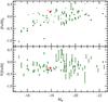 |
Fig. 5 Location of NGC 4486A in the metallicity and the metallicity gradients vs. luminosity diagrams. NGC 4486A is shown as red dots, and the other points are the galaxies from Koleva et al. (2011). |
Nowak et al. (2007) find that the velocity increases up to the edge of their field at 1.3″. At this point they note a rotation velocity of 115 ± 5 km s-1. We observe the peak at 2″ along the major axis, which is certainly consistent, given the difference of spatial resolution. Therefore, the peak of the rotation is reached between 1.3 and 2″, and the maximum rotation velocity is km s-1. The rotation velocity decreases monotically outwards.
4.3. NGC 4486A, a typical low-luminiosity elliptical
Figure 5 locates NGC 4486A in the metallicity and metallicity gradients vs. luminosity diagrams. The other galaxies represented in this figure are from Koleva et al. (2011).
NGC 4486A has a uniformly old population, a super-solar central metallicity, and a negative metallicity gradient ∇ [Fe/H ] = −0.24. These properties are similar to other galaxies in the same mass range. The orientation of the nuclear disk suggests that the galaxy is observed edge-on. The considerable rotation, implying Vmax/σ0 ≈ 1, is produced by a central concentration of mass and does not reflect a significant angular momentum.
The high h3 value, coinciding with the peak of rotation, indicates a population of fast rotating stars, and the steep decrease of the rotation in the external regions is consistent with the hypothesis proposed by Kormendy et al. (2005) for the formation of the disk. An ancient merger, 5 to 10 Gyr ago (because we do not see the effect on the population), injected some gas that cooled to the centre and formed a disk where it formed stars. This corresponds to the population observed in rotation, while the pre-existing population conserved a low rotation. However, because there is no signature in the stellar population, this scenario remains speculative.
4.4. Summary
We analysed long-slit spectra of NGC 4486A taken along its major axis and derived its internal kinematics, its age, and its metallicity. It is a typical low-luminosity elliptical galaxy.
We showed that with a careful composite modelling and a full-spectrum fitting it is possible to correct a galactic spectrum from the contamination by an external source of light and derive consistent information about the physical properties of the galaxy. The same approach can be used to separate a non-stellar emission in the nuclear region.
Acknowledgments
Ph.P. acknowledges the support from the Programe National Cosmologie et Galaxies (PNCG), INSU/CNRS. Ph.P. and W.Z. acknowlege a bilateral collaboration grant between France and Austria (AMADEUS, collaboration project PHC19451XM). S.d.R. and Ph.P.
acknowledge a bilateral collaboration grant between the Flander region and France (Tournesol). M.K. has been supported by the Programa Nacional de Astronomía y Astrofísica of the Spanish Ministry of Science and Innovation under grant AYA2007-67752-C03-01 and Bulgarian Scientific Research Fund DO 02-85/2008. She thanks CRAL, Observatoire de Lyon, Université Claude Bernard for an Invited Professorship. We thank Nina Nowak and the referee for comments on the manuscript.
References
- Bouchard, A., Prugniel, P., Koleva, M., & Sharina, M. 2010, A&A, 513, A54 [NASA ADS] [CrossRef] [EDP Sciences] [Google Scholar]
- de Vaucouleurs, G. H. 1959, Lowell Observatory Bulletin, 4, 105 [NASA ADS] [Google Scholar]
- de Vaucouleurs, G., & de Vaucouleurs, A. 1964, Reference catalogue of bright galaxies, ed. G. de Vaucouleurs, & A. de Vaucouleurs [Google Scholar]
- Koleva, M., Prugniel, P., Bouchard, A., & Wu, Y. 2009, A&A, 501, 1269 [NASA ADS] [CrossRef] [EDP Sciences] [Google Scholar]
- Koleva, M., Prugniel, P., de Rijcke, S., & Zeilinger, W. 2011, MNRAS, submitted [Google Scholar]
- Kormendy, J., Gebhardt, K., Fisher, D. B., et al. 2005, AJ, 129, 2636 [NASA ADS] [CrossRef] [Google Scholar]
- Kormendy, J., Fisher, D. B., Cornell, M. E., & Bender, R. 2009, ApJS, 182, 216 [NASA ADS] [CrossRef] [Google Scholar]
- Le Borgne, D., Rocca-Volmerange, B., Prugniel, P., et al. 2004, A&A, 425, 881 [NASA ADS] [CrossRef] [EDP Sciences] [Google Scholar]
- Makarova, L., Koleva, M., Makarov, D., & Prugniel, P. 2010, MNRAS, 406, 1152 [NASA ADS] [Google Scholar]
- Mei, S., Blakeslee, J. P., Côté, P., et al. 2007, ApJ, 655, 144 [NASA ADS] [CrossRef] [Google Scholar]
- Nowak, N., Saglia, R. P., Thomas, J., et al. 2007, MNRAS, 379, 909 [NASA ADS] [CrossRef] [Google Scholar]
- Nowak, N., Saglia, R. P., Thomas, J., et al. 2008, MNRAS, 391, 1629 [NASA ADS] [CrossRef] [Google Scholar]
- Prugniel, P., & Soubiran, C. 2001, A&A, 369, 1048 [NASA ADS] [CrossRef] [EDP Sciences] [Google Scholar]
- Prugniel, P., Nieto, J., & Simien, F. 1987, A&A, 173, 49 [NASA ADS] [Google Scholar]
- Prugniel, P., Soubiran, C., Koleva, M., & Le Borgne, D. 2007, New release of the ELODIE library: Version 3.1 [arXiv:astro-ph/0703658] [Google Scholar]
- Salpeter, E. E. 1955, ApJ, 121, 161 [Google Scholar]
- Schlegel, D. J., Finkbeiner, D. P., & Davis, M. 1998, ApJ, 500, 525 [NASA ADS] [CrossRef] [Google Scholar]
- Wegner, G., Bernardi, M., Willmer, C. N. A., et al. 2003, AJ, 126, 2268 [NASA ADS] [CrossRef] [Google Scholar]
- Wu, Y., Singh, H. P., Prugniel, P., Gupta, R., & Koleva, M. 2011, A&A, 525, A71 [NASA ADS] [CrossRef] [EDP Sciences] [Google Scholar]
All Tables
All Figures
|
Fig. 1 Central field of NGC 4486A. The location of the slit is superimposed on the composite image from Kormendy et al. (2005, their Fig. 4). The size is 8″ across. |
| In the text | |
|
Fig. 2 Radial profiles of NGC 4486A derived from SSP fits. The spectra are radially binned for a compromise between S/N and spatial resolution (they have at minimum S/N = 40). The profiles are folded around the position of the kinematical centre. The red points are for the positive radii (South side) and blue for negative; the tones separate the two setups (the darker colours are for the first setup). The abscissa is the position along the slit (a = x − 2.15). The vertical blue dashed line marks the effective isophote. From top to bottom the panels are: (1) the logarithm of the relative total flux; (2) the logarithm of 1/f; (3 to 7) the internal kinematics and the SSP-equivalent metallicity. The velocity and h3 of the north side (blue points) are symmetrized. The points with f < 0.5 were excluded. |
| In the text | |
|
Fig. 3 Fit of a spectrum of NGC 4486A. The top panel shows the observed (in black) and fitted (blue) spectra. The red points mark the excluded regions (because of strong telluric absorption) and the rejected pixels (kappa-sigma clipping). The two gaps between the detectors are visible near 4800 and 5750 Å. The middle panel shows the two components of the model separately, the galactic population in black, and the star in orange. The bottom panel presents the residuals (observation-model). The green lines are the 1-σ errors. |
| In the text | |
|
Fig. 4 Fit of the metallicity gradient. The colours are as in Fig. 2. The abscissa is the distance to the galaxy centre, divided by the effective semi-major axis. The straight line is the solution of the power-law fit, and its continuous region marks the used radial range. |
| In the text | |
|
Fig. 5 Location of NGC 4486A in the metallicity and the metallicity gradients vs. luminosity diagrams. NGC 4486A is shown as red dots, and the other points are the galaxies from Koleva et al. (2011). |
| In the text | |
Current usage metrics show cumulative count of Article Views (full-text article views including HTML views, PDF and ePub downloads, according to the available data) and Abstracts Views on Vision4Press platform.
Data correspond to usage on the plateform after 2015. The current usage metrics is available 48-96 hours after online publication and is updated daily on week days.
Initial download of the metrics may take a while.