| Issue |
A&A
Volume 528, April 2011
|
|
|---|---|---|
| Article Number | A98 | |
| Number of page(s) | 13 | |
| Section | Interstellar and circumstellar matter | |
| DOI | https://doi.org/10.1051/0004-6361/201015968 | |
| Published online | 08 March 2011 | |
The characterisation of irregularly-shaped particles
A re-consideration of finite-sized, “porous” and “fractal” grains
Institut d’Astrophysique Spatiale (IAS), Bâtiment 121, Université Paris-Sud
11 and CNRS,
91405
Orsay,
France
e-mail: This email address is being protected from spambots. You need JavaScript enabled to view it.
Received:
21
October
2010
Accepted:
15
January
2011
Abstract
Context. A porous and/or fractal description can generally be applied where particles have undergone coagulation into aggregates.
Aims. To characterise finite-sized, “porous” and “fractal” particles and to understand the possible limitations of these descriptions.
Methods. We use simple structure, lattice and network considerations to determine the structural properties of irregular particles.
Results. We find that, for finite-sized aggregates, the terms porosity and fractal dimension may be of limited usefulness and show with some critical and limiting assumptions, that “highly-porous” aggregates (porosity ≳80%) may not be “constructable”. We also investigate their effective cross-sections using a simple “cubic” model.
Conclusions. In place of the terms porosity and fractal dimension, for finite-sized aggregates, we propose the readily-determinable quantities of inflation, I (a measure of the solid filling factor and size), and dimensionality, D (a measure of the shape). These terms can be applied to characterise any form of particle, be it an irregular, homogeneous solid or a highly-extended aggregate.
Key words: dust, extinction
© ESO, 2011
1. Introduction
Interstellar, interplanetary or cometary dust particles are generally modelled as spheres, or collections of mono- or multi-disperse spheres. Such approaches are clearly rather idealised starting points from which to model and to perform analogue experiments aimed at understanding the obviously much more complex and diverse forms of dust in astrophysical media. For example, many of the collected interplanetary dust particles, or IDPs, show complex, extended and open structures comprised of aggregates of irregular sub-grains with radii typically of the order of hundreds of nanometres (e.g., Brownlee 1978; Rietmeijer 1998). Such types of structures are to be expected in coagulated grains in interstellar and proto-planetary disc particles (e.g., Ossenkopf 1993; Ormel et al. 2007, 2009) and are seen in soot particle experiments and simulations (e.g., Dobbins & Megaridis 1991; Köylü et al. 1995; Mackowski 2006, and references therein).
Highly-porous grains, of apparently arbitrarily-large porosity, can be constructed mathematically but can they exist physically, i.e., can we build a physical 3D model of them and do such particles bear any resemblance to “real” interstellar grains? Such particles also pose the question as to how one should define porosity in these cases.
In this paper we discuss the issues of aggregate/irregular grain porosity and fractal structure and attempt to define characteristic properties for aggregate grains, composed of single-sized spherical constituent grains (also known as sub-grains or primary particles) that can be determined using simple measures of the aggregate geometry. We show that this approach can be extended to any irregularly-shaped particle.
2. Porosity matters
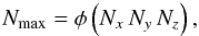
The porosity, P, of a particle is usually defined as,
 (1)where
Vv and Vs are the volumes of
vacuum and of the solid matter making up the particle, and Vt is
the total volume of the particle within some defined surface. Note that this definition of
porosity is independent of the form of the particles, which can be of any arbitrary shape,
and is only defined for 0 ≤ P < 1. The problem with
this definition of porosity is that it is often difficult to define a physically-reasonable
surface that delimits the particle in an unequivocal way. Clearly, a measure of a particle’s
porosity requires an unambiguous definition of the reference volume, which
is in many, if not most, cases not possible. Thus, the porosity of very extended particles
can be hard to define and it may not make much sense to talk of “highly porous” particles.
It therefore seems that a better measure or a more open-ended definition of the nature of
coagulated grains is needed. Ormel et al. (2007,
2009) have considered the “porosity” of coagulated
grains in terms of an enlargement parameter and a geometrical filling factor approach to
determine the particle cross-sections, respectively. We return to a discussion of these
ideas later.
(1)where
Vv and Vs are the volumes of
vacuum and of the solid matter making up the particle, and Vt is
the total volume of the particle within some defined surface. Note that this definition of
porosity is independent of the form of the particles, which can be of any arbitrary shape,
and is only defined for 0 ≤ P < 1. The problem with
this definition of porosity is that it is often difficult to define a physically-reasonable
surface that delimits the particle in an unequivocal way. Clearly, a measure of a particle’s
porosity requires an unambiguous definition of the reference volume, which
is in many, if not most, cases not possible. Thus, the porosity of very extended particles
can be hard to define and it may not make much sense to talk of “highly porous” particles.
It therefore seems that a better measure or a more open-ended definition of the nature of
coagulated grains is needed. Ormel et al. (2007,
2009) have considered the “porosity” of coagulated
grains in terms of an enlargement parameter and a geometrical filling factor approach to
determine the particle cross-sections, respectively. We return to a discussion of these
ideas later.
3. Fractal matters
We recall that a fractal structure has the property of self-similarity and that the
constituent parts of its structure can be considered a reduced copy of the whole, i.e., the
details of the structure are essentially scale- or reference point-invariant. The
characteristic of a fractal structure is its Rényi, Hausdorff or packing dimension (i.e.,
the fractal dimension). In a rather general way the fractal dimension,
Df, of a system can be defined as follows:
 (2)where
N(r) and M(r) are the
number and mass, respectively, of particles within a defined radius, r,
from a given reference point. This definition of the fractal dimension, or what might
perhaps be called the “fractality” of the system, is determined by the spatial distribution
of the structural units existing within a defined spherical volume of a much larger entity.
For an infinitesimally-reducible structure, such as the Mandelbrot set, this clearly poses
no problem. However, for a finite sized, porous particle, which does not exist beyond this
assumed spherical volume and does not reproduce itself at ever smaller size-scales, the idea
of a scale-invariant fractal dimension no longer holds. Interstellar grains therefore cannot
be fractal in the true sense of the definition of fractal entities because their structures
are not scale-invariant, i.e., a shift in the reference point will not always yield the same
fractal dimension. For example, a finite piece of “chicken wire” (essentially a 2D hexagonal
grid or mesh) might be considered to have a fractal dimension of two globally but one
locally when one descends to the level of the wire and no longer sees the larger mesh. Thus,
the use of the term fractal, when referring to finite-sized particles, can be rather
misleading. It would seem that a better description for irregular interstellar grains ought
to be possible and should be rather general.
(2)where
N(r) and M(r) are the
number and mass, respectively, of particles within a defined radius, r,
from a given reference point. This definition of the fractal dimension, or what might
perhaps be called the “fractality” of the system, is determined by the spatial distribution
of the structural units existing within a defined spherical volume of a much larger entity.
For an infinitesimally-reducible structure, such as the Mandelbrot set, this clearly poses
no problem. However, for a finite sized, porous particle, which does not exist beyond this
assumed spherical volume and does not reproduce itself at ever smaller size-scales, the idea
of a scale-invariant fractal dimension no longer holds. Interstellar grains therefore cannot
be fractal in the true sense of the definition of fractal entities because their structures
are not scale-invariant, i.e., a shift in the reference point will not always yield the same
fractal dimension. For example, a finite piece of “chicken wire” (essentially a 2D hexagonal
grid or mesh) might be considered to have a fractal dimension of two globally but one
locally when one descends to the level of the wire and no longer sees the larger mesh. Thus,
the use of the term fractal, when referring to finite-sized particles, can be rather
misleading. It would seem that a better description for irregular interstellar grains ought
to be possible and should be rather general.
As we will show low Df particles cannot be “porous” because this leads to a loss of continuity in the structure. Thus, the “fractal” nature of a structure is coupled to its “porosity” and the two properties therefore cannot be independently varied, as already discussed in some detail by Mandelbrot (1982).
4. Sparse lattices
By sparse lattice we here mean stacked constituents on a regular lattice (e.g., cubic, hexagonal or face-centred cubic) in which not every lattice site is necessarily occupied.
4.1. Simple cubic lattices
A simple cubic lattice, i.e., a lattice composed of equi-dimensional regular cubic constituents, can be packed together with 100% efficiency leaving no intervening, unfilled space. This lattice is clearly not of relevance to the structure of interstellar grains but it does, nevertheless, provide some useful intuitive insight into the nature of porous grain structures.
In a simple cubic lattice each site shares 6 faces, 12 edges and 8 corners with
neighbouring lattice sites. If we now randomly remove lattice sites we can look at how the
number of neighbouring sites depends on the porosity. For illustrative purposes we
consider constituent cubes of edge length l stacked into a cubic particle
of edge length nl (i.e., total number of lattice sites
= n3). A cubic particle of porosity P then
contains (1 − P)n3 occupied sites and the
average number of occupied adjacent sites (ignoring the macroscopic particle outer edges
and surfaces), which we call the coordination number for a given porosity,
CP, is simply
(1 − P)C, where C is the maximum site
coordination number under consideration. For a cubic lattice, C may take
the values 6, 18 or 26, depending on the hierarchy of the coordination that we allow,
i.e., sites sharing only faces (C = 6), sites sharing faces and edges
(C = 6 + 12 = 18) sites sharing faces, edges and corners
(C = 6 + 12 + 8 = 26). We then have that
 (3)We are now
interested in the limit where the structure is just continuous and, therefore, can be
physically constructed as a single entity. Two limits are of interest here:
(3)We are now
interested in the limit where the structure is just continuous and, therefore, can be
physically constructed as a single entity. Two limits are of interest here:
-
1.
the dimer limit where each site has only one occupiedneighbouring site and the system therefore consists only ofdimers. Such a “structure” is clearly not macroscopic, does not“hold up” and is not “constructable”;
- 2.
the continuity limit, which is somewhat akin to the percolation threshold for a lattice, where the structure is just bound into a single, “one-dimensional” unit by inter-site contacts or bonds.
The first case is trivial and CP = 1. The second case is of interest in determining whether a given structure is “constructable” and in this case CP is just equal to 2, which ensures that the network can, minimally, completely inter-link. In this case each site has two filled neighbouring sites and the network can, in theory at least, propagate over the whole considered volume as a 1D “chain”. Although, in the latter case the structure would resemble something like a ball of wire, i.e., a one-dimensional construct warped into a three dimensional space, which is not a fractal structure.
For the simple cubic lattice, or in fact for any lattice, the relevant critical
porosities Pcrit for a given case are given by
 (4)For the dimer
limit, i.e., CP = 1, we then have
that
(4)For the dimer
limit, i.e., CP = 1, we then have
that  ,
respectively, for the C = 6, 18 and 26 maximum coordination cases. For
the more interesting continuity limit case, where
CP = 2, we have
,
respectively, for the C = 6, 18 and 26 maximum coordination cases. For
the more interesting continuity limit case, where
CP = 2, we have
 ,
respectively, for the C = 6, 18 and 26 maximum coordination cases. In
the latter case, i.e. C = 26, allowing a structure to coordinate only
through the corner points is perhaps a rather extreme situation. The equivalent porosities
for the three cases are ≈66, 89 and 92%. For comparison, percolation theory, see for
example Stauffer & Aharony (1994), predicts
site and bond percolation thresholds of 0.3116 and 0.2488, respectively, which would be
equivalent to “critical porosities” of ≈69 and 75%. Our simple model therefore indicates
values roughly consistent with percolation theory.
,
respectively, for the C = 6, 18 and 26 maximum coordination cases. In
the latter case, i.e. C = 26, allowing a structure to coordinate only
through the corner points is perhaps a rather extreme situation. The equivalent porosities
for the three cases are ≈66, 89 and 92%. For comparison, percolation theory, see for
example Stauffer & Aharony (1994), predicts
site and bond percolation thresholds of 0.3116 and 0.2488, respectively, which would be
equivalent to “critical porosities” of ≈69 and 75%. Our simple model therefore indicates
values roughly consistent with percolation theory.
4.2. Close-packed lattices
We now turn our attention to the perhaps more astrophysically-relevant, but still idealised, case of close-packed lattices of spherical entities. In this case we note that the lattice positions are fixed and that the constituent “monomers” cannot take arbitrary positions. Nevertheless, this is a useful starting point.
By simple close-packed lattices we refer to lattices composed of regular, equal-sized
spheres packed as efficiently as possible, i.e., face-centred cubic (fcc) and hexagonal
close packing (hcp), which are identical for our purposes. However, for the simplicity of
the presentation, we will only consider the fcc case for simple solid spheres. For
identical size and composition spheres, the fcc lattice unit cell can be considered as a
cube where each face of the cube shares a sphere with one adjacent unit cell and each
corner of the cube shares a sphere with seven other neighbouring unit cells. It then
follows that each fcc unit cell contains  spheres
within a cube of side length
spheres
within a cube of side length  where
d is the diameter of the sphere. The volume of the cube is then
where
d is the diameter of the sphere. The volume of the cube is then
 (5)and
the volume occupied by the solid matter of the spheres is
(5)and
the volume occupied by the solid matter of the spheres is
 (6)The porosity of
such a vacancy- or defect-riddled fcc structure is then given by
(6)The porosity of
such a vacancy- or defect-riddled fcc structure is then given by
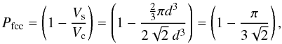 (7)i.e., a porosity of 26%,
which is equivalent a solid filling factor of
(7)i.e., a porosity of 26%,
which is equivalent a solid filling factor of  , which appears to be the
most efficient lattice packing possible for equal-sized spheres. The same value holds for
the hcp lattice. For the simple cubic packing of spheres it can similarly be shown that
the filling factor is
, which appears to be the
most efficient lattice packing possible for equal-sized spheres. The same value holds for
the hcp lattice. For the simple cubic packing of spheres it can similarly be shown that
the filling factor is  . These results can be
found in standard textbooks on crystallography and the solid state.
. These results can be
found in standard textbooks on crystallography and the solid state.
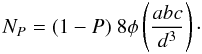
We now consider a spherical volume of radius A and volume
Vg, perhaps equivalent to an aggregate interstellar grain,
composed of spherical sub-grains, of volume Vsg, packed on a
fcc lattice. The maximum number of sub-grains, Nmax, within
the total grain volume is then 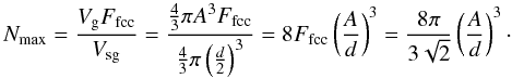 (8)We now use the above
results to study the effects of introducing porosity into the structure by removing some
of the sub-grains from the lattice. If N is the total number of
sub-grains within the particle or aggregate
(N ≤ Nmax) then, following from the
definition above (with
(8)We now use the above
results to study the effects of introducing porosity into the structure by removing some
of the sub-grains from the lattice. If N is the total number of
sub-grains within the particle or aggregate
(N ≤ Nmax) then, following from the
definition above (with  ), the porosity
of the particle is given by
), the porosity
of the particle is given by ![Mathematical equation: \begin{equation} P = \left( 1 - \frac{ N \frac{\pi}{6} d^3}{ \frac{4}{3} \pi A^3 \ F_{\rm fcc} } \right) = \left[ 1 - N \left( \frac{d}{A} \right)^3 \frac{3 \sqrt{2}}{8 \pi} \right] = \left( 1 - \frac{N}{N_{\rm max}} \right), \end{equation}](/articles/aa/full_html/2011/04/aa15968-10/aa15968-10-eq52.png) (9)or, equivalently, the
number of sub-grains for a given porosity,
NP, is given by
(9)or, equivalently, the
number of sub-grains for a given porosity,
NP, is given by
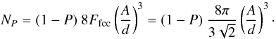 (10)where we recover the
value Nmax when P = 0.
(10)where we recover the
value Nmax when P = 0.
The average sub-grain coordination number for our porous lattice, which can be expressed
in the same way as for the simple cubic lattice discussed above, is simply the maximum
coordination number, C (12 for fcc and hcp), multiplied by the fraction
of filled sites (1 − P), i.e.,
CP = (1 − P)C.
In this case the dimer limit and continuity limit
critical porosities, Pcrit, are
 and
and
 , i.e.,
92% and 83%, respectively. Thus, it appears that, for this idealised close-packed lattice
(fcc or hcp) model, there is an upper limit to the porosity of a particle and that this
limit is ≈80%. For the cubic lattice the equivalent limiting porosity is ≈70%. Note
that these limits are given by (1 − [2/C]) and are
therefore independent of the monomer size.
, i.e.,
92% and 83%, respectively. Thus, it appears that, for this idealised close-packed lattice
(fcc or hcp) model, there is an upper limit to the porosity of a particle and that this
limit is ≈80%. For the cubic lattice the equivalent limiting porosity is ≈70%. Note
that these limits are given by (1 − [2/C]) and are
therefore independent of the monomer size.
However, remember that this limiting porosity strongly depends upon the above, and widely
used, definition of porosity and the fixed lattice positions for our particle subgrains.
It also depends on the fact that we have assumed that the sub-grains are “evenly”
distributed throughout the volume  . We now look at the
nature and definition of porosity more closely.
. We now look at the
nature and definition of porosity more closely.
5. Sparse networks
By sparse network we here mean contiguous, irregularly-connected, spherical constituents that do not lie on a regular lattice.
5.1. General packing of spherical grains
We consider a mono-disperse collection of connected spherical sub-grains in an
arbitrarily-shaped, “porous” particle that can be defined by its three semi-major axes
(a,b and c), as per an ellipsoid, with an “enclosing”
volume,  . The
maximum number of sub-grains of diameter d within this assumed volume is
given by
. The
maximum number of sub-grains of diameter d within this assumed volume is
given by 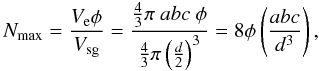 (11)similar to that defined
for a spherical particle above but where we have now replaced the maximum fcc lattice
packing efficiency for mono-disperse, spherical particles,
(11)similar to that defined
for a spherical particle above but where we have now replaced the maximum fcc lattice
packing efficiency for mono-disperse, spherical particles,
 , by a
more-generalised maximum packing efficiency φ. The porosity of the
particle is given by
, by a
more-generalised maximum packing efficiency φ. The porosity of the
particle is given by ![Mathematical equation: \begin{equation} P = \left( 1 - \frac{ N \ \frac{\pi}{6} d^3}{ \frac{4}{3} \pi \ a b c \ \phi } \right) = \left[ 1 - \frac{N}{8 \phi} \left( \frac{d^3}{a b c} \right) \right] = \left( 1 - \frac{N}{N_{\rm max}} \right), \end{equation}](/articles/aa/full_html/2011/04/aa15968-10/aa15968-10-eq71.png) (12)and the number of
sub-grains for a given porosity, NP, is
(12)and the number of
sub-grains for a given porosity, NP, is
 (13)We can now consider a
more generalised definition of the semi-major axes, a,b and
c, of our porous particle that is independent of the filling factor. We
normalise the three principal axes of the particle (i.e., 2a,
2b and 2c) by the monomer size, d. If
we assume that these axes are parallel to the Cartesian axes x,y and
z, and that
Nx = 2a/d, Ny = 2b/d
and
Nz = 2c/d,
then the volume within the encompassing surface is
(13)We can now consider a
more generalised definition of the semi-major axes, a,b and
c, of our porous particle that is independent of the filling factor. We
normalise the three principal axes of the particle (i.e., 2a,
2b and 2c) by the monomer size, d. If
we assume that these axes are parallel to the Cartesian axes x,y and
z, and that
Nx = 2a/d, Ny = 2b/d
and
Nz = 2c/d,
then the volume within the encompassing surface is 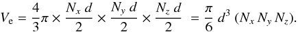 (14)We can simplify the
above expressions for Nmax, P and
NP to:
(14)We can simplify the
above expressions for Nmax, P and
NP to:
 (15)
(15)![Mathematical equation: \begin{equation} P = \left[ 1 - \frac{1}{\phi } \left( \frac{N}{N_x \, N_y \, N_z} \right) \right] = \left( 1 - \frac{N}{N_{\rm max}} \right), \end{equation}](/articles/aa/full_html/2011/04/aa15968-10/aa15968-10-eq82.png) (16)
(16) (17)The key parameters in
defining our arbitrary particle are now the number of constituent monomers,
N, and its normalised dimensions,
Nx,Ny
and Nz or more generally
Ni where
i = x,y or z. The nature of the
particle can be characterised, independent of porosity or fractal measures, through the
sum, Σi, and the product, Πi, of
its dimensions, i.e.,
(17)The key parameters in
defining our arbitrary particle are now the number of constituent monomers,
N, and its normalised dimensions,
Nx,Ny
and Nz or more generally
Ni where
i = x,y or z. The nature of the
particle can be characterised, independent of porosity or fractal measures, through the
sum, Σi, and the product, Πi, of
its dimensions, i.e., 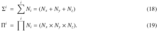 Table 1 shows the values of Σi
and Πi for the most compact and the most extended particles
possible. For highly porous “disc-like” and “sphere-like” distributions this corresponds
to linear structures located along 2 and 3 orthogonal axes, respectively. Note that a
one-dimensional or rod-like assemblage of spheres can never be porous since any “vacancy”
cuts the structure into smaller but separated particles. Thus, the maximum possible
particle dimension is Nd and the minimum particle dimension is that of
the most compact spherical particle possible, i.e.,
φN1/3d.
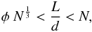
Figure 1 shows the relationship between
Σi and Πi as a function of the
particle dimensionality, which is defined below.
Table 1 shows the values of Σi
and Πi for the most compact and the most extended particles
possible. For highly porous “disc-like” and “sphere-like” distributions this corresponds
to linear structures located along 2 and 3 orthogonal axes, respectively. Note that a
one-dimensional or rod-like assemblage of spheres can never be porous since any “vacancy”
cuts the structure into smaller but separated particles. Thus, the maximum possible
particle dimension is Nd and the minimum particle dimension is that of
the most compact spherical particle possible, i.e.,
φN1/3d.
Figure 1 shows the relationship between
Σi and Πi as a function of the
particle dimensionality, which is defined below.
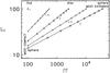 |
Fig. 1 Axis sum, Σi, vs. axis product, Πi, plot for a particle containing 100 identical sub-particles as a function of the dimensionality (as indicated): D = 1 (diamond), 1.5 (plus signs), 2 (triangles), 2.5 (crosses) and 3 (squares). Compact particles are to the lower left and extended particles to the upper right. Note that no porosity is allowed for D = 1, rod-like particles. |
Σi and Πi for compact and highly extended particles.
We can see from Table 1 that for the most compact
particles Σi ≤ N and
Πi = N and for the most extended particles
Σi = N and
Πi ≥ N. If we wish we can consider the
porosity, P, of these particles and re-write
Nmax, P and
NP as:
 (20)
(20) (21)
(21) (22)However, the advantage of
using the Σi and Πi
characterisation is that we have a system that can generically describe an
arbitrarily-extended particle without the need to define its porosity or its “fractality”.
(22)However, the advantage of
using the Σi and Πi
characterisation is that we have a system that can generically describe an
arbitrarily-extended particle without the need to define its porosity or its “fractality”.
5.2. Dimensionality and inflation
With a view to generalising the notion of grain “porosity”, or better characterising
extended particles, we consider a more open-ended definition than simply the particle
porosity, as did Ormel et al. (2007, 2009). Ormel et al.
(2007) considered grains in terms of an enlargement parameter, the ratio of the
extended volume to the most compact volume. Whereas Ormel
et al. (2009) used a geometrical filling factor approach to determine the
particle cross-sections. We now consider the idea of particle “inflation” beyond the most
compact forms possible. In this case we define the inflation, I, for a
given particle as: 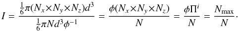 (23)Inflation is thus,
equivalently, the ratio of the volume of the enclosing ellipsoid
(
(23)Inflation is thus,
equivalently, the ratio of the volume of the enclosing ellipsoid
( , Eq. (14)) to the (minimum) volume of the solid
matter in the aggregate (
, Eq. (14)) to the (minimum) volume of the solid
matter in the aggregate (![Mathematical equation: \hbox{$\frac{4}{3} \pi \, [N^{\frac{1}{3}}]^3 \, (d/2)^3 \ \phi^{-1} = \frac{1}{6} \pi \, N \, d^3 \ \phi^{-1}$}](/articles/aa/full_html/2011/04/aa15968-10/aa15968-10-eq115.png) ),
where φ is the maximum packing efficiency of the sub-grains in the
minimum volume. For cubic particles (on a cubic grid, see Sect. 4.1), where φ = 1, we have
),
where φ is the maximum packing efficiency of the sub-grains in the
minimum volume. For cubic particles (on a cubic grid, see Sect. 4.1), where φ = 1, we have
 . Note that with this
definition an inflation factor I = 10 could be considered akin to a
porosity of 90%.
. Note that with this
definition an inflation factor I = 10 could be considered akin to a
porosity of 90%.
The inflation, I, for any particle has a minimum value of unity and a maximum value of ≈N2/27 (for unit packing efficiency, i.e., φ = 1), which is determined by the most-extended “spherical” particle possible. This hypothetical, and rather physically unrealistic, structure has an equal number of sub-particles (N/3) arranged along the three orthogonal, cartesian axes. This corresponds to the extreme upper right part of Fig. 1. For a particle with a dimensionality of 2 the maximum value of I is ≈N/4. We can see that with this definition the increase in the particle size by a factor of f translates to an inflation factor of f3, provided that the condition (Nx + Ny + Nz) ≤ N is fulfilled. Note that the largest values of I are to be found for the most “spherical” extended particles where the product, Πi, is a maximum for a given sum, Σi.
We now define the dimensionality, D, of any given extended particle in
terms of its maximum-dimension-normalised sum Σi:
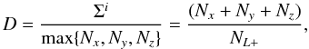 (24)where
NL + = max { Nx,Ny,Nz }
and indicates that we take the longest dimension of the particle, as the normalisation
length.
(24)where
NL + = max { Nx,Ny,Nz }
and indicates that we take the longest dimension of the particle, as the normalisation
length.
It is clearly possible to extend this definition of D to the general
case of any arbitrary-shaped particle, independent of whether it is an aggregate or a
highly irregular single “lump”, i.e.,
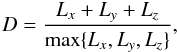 (25)where
Li is the particle size along its
ith axis (x, y or
z). As an illustrative example, in Table 2 we show the dimensionality and inflation factors for several regular solids,
where the value Lx
(Lz) is, generally, the maximum (minimum)
dimension of the regular solid. Note that in the case of the cube the longest dimension,
Lx, is the cube diagonal, and not an edge,
and that the other two dimensions are then taken orthogonal to this direction.
(25)where
Li is the particle size along its
ith axis (x, y or
z). As an illustrative example, in Table 2 we show the dimensionality and inflation factors for several regular solids,
where the value Lx
(Lz) is, generally, the maximum (minimum)
dimension of the regular solid. Note that in the case of the cube the longest dimension,
Lx, is the cube diagonal, and not an edge,
and that the other two dimensions are then taken orthogonal to this direction.
The dimensionality, D, and inflation, I, for regular geometrical solids. a and l are the relevant radius and side/edge lengths, respectively.
For our general case we can define a minimum and a maximum particle dimension,
NL − and
NL + , respectively, defined by the
minimum volume (spherical) close-packed particle, of radius a, and the
maximum linear chain length. These extreme particle dimensions are given, for the fcc
close-packed and the more general case, by
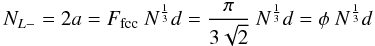 (26)and
 (27)Thus, all possible
particles must have sizes, L (expressed in terms of the sub-unit
dimension d), within the range
(27)Thus, all possible
particles must have sizes, L (expressed in terms of the sub-unit
dimension d), within the range
 (28)where the lower limit
can be equated with a fractal dimension Df ≈ 3 and the upper
limit with Df ≈ 1. However, the particles in question are not
necessarily “truly” fractal in nature. In fact, this definition of the quantity
dimensionality (1 ≤ D ≤ 3) can indeed be applied to any particle, whether
solid and homogeneous (I = 1), particles with concavities and protrusions
or porous aggregates (I > 1). Additionally, the
concept of inflation can be applied to any particle because it is just the volume of the
enclosing ellipsoid, that can directly determined from the particle dimensions, divided by
the minimum volume of the solid matter
(Vs/φ, where
φ is set to the maximum packing efficiency and is set to 1 for a solid
particle).
(28)where the lower limit
can be equated with a fractal dimension Df ≈ 3 and the upper
limit with Df ≈ 1. However, the particles in question are not
necessarily “truly” fractal in nature. In fact, this definition of the quantity
dimensionality (1 ≤ D ≤ 3) can indeed be applied to any particle, whether
solid and homogeneous (I = 1), particles with concavities and protrusions
or porous aggregates (I > 1). Additionally, the
concept of inflation can be applied to any particle because it is just the volume of the
enclosing ellipsoid, that can directly determined from the particle dimensions, divided by
the minimum volume of the solid matter
(Vs/φ, where
φ is set to the maximum packing efficiency and is set to 1 for a solid
particle).
Clearly any given, finite-sized particle can only have dimensionalities in the range 1 to 3. The dimensionality, D, when coupled to I, can perhaps be considered as somewhat analogous to the fractal dimension of a structure and as a representation of the spatial arrangement.
The concepts of porosity and fractal structure (“fractality”) for any given extended and “constructable” particle can now re-posed in terms of the related and estimable quantities of inflation (I) and dimensionality (D). In Fig. 2 we show a plot of D vs. I for ≈15 000 randomly-generated particles containing 50 identical sub-grains. For illustrative purposes we have assumed maximum packing efficiency (i.e., φ = 1). These aggregates were generated by imposing the conditions: 1 ≤ Ni ≤ N (where i = x, y or z), Σi ≤ N and Πi ≥ N. From this figure it appears that particles created in this way are dominated by dimensionalities of the order of ≈1.2–2.3 and inflation factors of ≈5–50. The lower cut-off to the data points in this figure is simply due to the relationship between the sum of the particle dimensions, which determines the maximum dimension and therefore D, and the product of the particle dimensions, which determines the volume and hence I.
In Fig. 2 all particles are assumed to be equally “constructable”. However, given that the number of possible structural isomers for the given number of monomers (that we could perhaps call “structomers”) must increase with the enclosing volume Ve, the more extended structures are given undue weight in Fig. 2. This is indicated by the higher density of the data points for larger values of I in this linear-log plot. Hence, and for illustrative purposes, in Fig. 3 we plot another simulation in which the size of the data points are volume-weighted by dividing by I and shape-weighted by multiplying by (1 − [Dm − 2]2). For the shape-weighting we adopt an illustrative mean value of the dimensionality Dm = 2, i.e., close to the typical fractal dimension (i.e., Df = 1.8) seen in soot particle formation experiments. What Fig. 3 shows is that, assuming Dm = 2, aggregate particles will probably have inflation factors I < 10. However, this will obviously require a more detailed investigation than presented here because the “structomer” distribution in the D vs. I parameter space will depend upon the adopted particle construction protocol.
Thus, what emerges from the above is that it is perhaps not the fractal dimension or even the porosity that counts for finite-sized, extended particles but the “dimensionality” of the structure coupled to its “inflation”. In Table 1 we can see that the “dimensionality” is represented in the exponents of Σi and Πi.
 |
Fig. 2 Dimensionality, D, versus inflation, I, plot for particles containing 50 equal-sized constituents for ≈15 000 randomly-generated structures (with φ = 1). The inset box shows the limits on D (1 ≤ D ≤ 3) and I (1 ≤ I ≤ N2/27), and the middle vertical line shows the limit for an idealised 2D particle, i.e., I = N/4. |
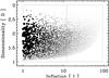 |
Fig. 3 Same as for Fig. 2 except that we have now volume- and shape-weighted the data point sizes by a factor (1 − [D − 2]2)/I (see text). |
In Appendix A we consider the implications of the above characterisation of irregular particles for the calculation of their cross-sections.
6. Implications for astronomical dust studies
Perhaps in no small part motivated by the then rather recent publication of the Bohren & Huffmann (1983) book, early studies of “porous” and composite interstellar grains, which must implicitly be irregular in form, treated “porosity” as vacuum filling a given fraction of the particle “volume” but did not take into account effects arising from their irregular structure (e.g., Jones 1988; Mathis & Whiffen 1989). These early investigations of grain porosity, and those subsequent to them, adopted a variety of approaches to the problem, including: effective medium theories (EMT, e.g., Jones 1988; Mathis & Whiffen 1989), hollow spheres (HS, e.g., Jones 1988; Min et al. 2005), multi-layered sphere models (MLS, e.g., Voshchinnikov et al. 2005) and discrete dipole approximations such as DDA (e.g., Bazell & Dwek 1990; Perrin & Sivan 1990, 1991; Henning & Stognienko 1993; Wolff et al. 1994). These methods can be put into three general classes: 1) implicit orientation-averaged (HS and MLS – spherical shell representations of an infinite number of randomly-orientated structures), 2) optical property averaged methods (EMT – solid “dilution” by the addition of vacuum, e.g., see Appendix B), and 3) fixed-shape methods where orientation- and structure-averaging is required (DDA). Comparison studies (e.g., Jones 1988; Wolff et al. 1994, 1998; Voshchinnikov et al. 2005; Shen et al. 2008, 2009) reveal that the results of these very different methods actually compare rather well. However, the “averaged” approach EMT, HS and MLS methods, as applied to spheroidal porous grains, cannot account for the details of the scattering properties of porous/irregular particles. In this sense DDA-generated particle studies do a much better job in determining the scattering properties of porous particles (e.g., Shen et al. 2008, 2009) because they take into account shape effects. Recently (Skorov et al. 2010, and their earlier work cited therein) studied very large, fluffy aggregates (N ≲ 2000) and conclude that their optical properties are sensitive to the aggregate size parameter, that characterisation by only N is insufficient (i.e., more detailed descriptions are needed) and that polarisation data can provide a measure of the aggregate fluffiness.
The concepts of inflation, I, and dimensionality, D, as defined here, can be applied to any arbitrary-shaped particle that is “constructable” with the DDA approach. They can also be applied to aggregates of spherical primary particles or monomers that can be analysed with the T-matrix method (TMM, e.g., Mackowski & Mishchenko 1996) and the generalised multiparticle Mie theory method (GMM, e.g., Xu 1995). All such particles are characterisable in terms of I and D. The “porosity” of very open structures (i.e., “highly porous” particles) is not unambiguously determineable, for the reasons discussed in the earlier sections, and the “fractal dimension” description for aggregates consisting of a rather limited number of monomers or primary particles does not appear tenable (see earlier sections and also Köhler et al. 2011).
The D and I descriptors may be particularly useful for characterising highly elongated structures and more meaningful than is possible with a porous particle description. Elongated structures actually correspond to low values of D and, perhaps rather surprisingly, also to low values of I. The low values of I arise in this case because the enclosing ellipsoid surface lies close to most of the constituent sub-particles because of its “cigar” shape.
In a porous aggregate the projected cross-section can be significantly less than that adopted in the “averaged” and “dilution” methods (e.g., EMT, HS and MLS) where the particle is assumed to be spherical and defined by a porosity-weighted, effective radius (e.g., see Appendix A.1). In the determination of the optical properties these methods actually do a surprisingly good job. In Appendices B and C we present some aspects of the Bruggemann EMT methods and dust cross-sections at long wavelengths that could be useful in studies of inhomogeneous particle studies.
6.1. Irregular particle mean projected cross-sections
We now use the methods developed earlier, to explore the relationship between
D and I, to estimate the projected cross-sections of
randomly-constructed aggregates within an ellipsoidal volume. For this exploratory model
we use 81 cubic primary particles (i.e., N = 81) on a cubic grid (see
Sect. 4.1), which have unit packing efficiency
(φ = 1) and a “spherical” compact form with cube centres that lie
within a circumscribed sphere of diameter 5 times the length of the side of a cube. As
before, the values of D and I for the particles are
randomly generated. The centre of each face of the
Nx × Ny × Nx
“box” that encompasses the ellipsoid is assigned a primary particle, and this used as a
seed to link the faces with randomly-generated but sequentially-coordinated primary cubes.
This ensures that the values of D and I so-generated are
fulfilled for the particle in question. Extra cubes are added, randomly but also
sequentially-coordinated to existing particle cubes, until the aggregate contains the
required 81 primary particles. The coordination number,
mi, for each cubic element
i in the generated aggregate is calculated by summing the number of
occupied nearest neighbour cubes. The mean coordination number for each generated
aggregate is then  .
The minimum condition for a constructable, single particle is the continuity limit for the
cubic lattice, i.e.,
.
The minimum condition for a constructable, single particle is the continuity limit for the
cubic lattice, i.e.,  (see Sect. 4.1) and aggregates with
 are therefore rejected. In constructing an aggregate we only allow neighbour-coordination
by cube faces and edges (see Sect. 4.1), which
corresponds to the condition
are therefore rejected. In constructing an aggregate we only allow neighbour-coordination
by cube faces and edges (see Sect. 4.1), which
corresponds to the condition  .
However, coordination numbers up to 26 are, in principle, possible because of the random
filling method used. For the aggregates
.
However, coordination numbers up to 26 are, in principle, possible because of the random
filling method used. For the aggregates  is always greater than 2, and generally less than 4 for these sparse lattices.
In Fig. 4 we show a D vs.
I plot for a limited range of I (≤10). The symbols
(filled circles) are size-scaled by the mean particle coordination number
,
which lies in the range  .
The crosses indicate “particles” with
that are not constructable (see Sect. 4.1) and
therefore eliminated from the cross-section analysis. Note that most of the rejected
particles “envelope” the valid aggregates at higher values of I. The
values of
are not systematically distributed in the D vs. I space
but appear to be somewhat random. Also note that the majority of the constructable
aggregates have I < 5, which correspond to
porosities ≲80%. The curved series of data points for the valid aggregates, especially
visible at the lower values of I are due to the discreteness, in the
limited range of compact aggregates for N = 81, and the coupling between
D and I (see below).
.
The crosses indicate “particles” with
that are not constructable (see Sect. 4.1) and
therefore eliminated from the cross-section analysis. Note that most of the rejected
particles “envelope” the valid aggregates at higher values of I. The
values of
are not systematically distributed in the D vs. I space
but appear to be somewhat random. Also note that the majority of the constructable
aggregates have I < 5, which correspond to
porosities ≲80%. The curved series of data points for the valid aggregates, especially
visible at the lower values of I are due to the discreteness, in the
limited range of compact aggregates for N = 81, and the coupling between
D and I (see below).
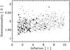 |
Fig. 4 The same as Fig. 3 but for ≈500 aggregates
(consisting of 81 cubic primary particles) and a more limited range of
I (≤10). The symbols (filled circles) are size-scaled by
|
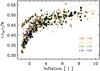 |
Fig. 5 The effective cross-section, normalised to the number of primary particles, N, for ≈500 aggregates constructed from 81 cubic primary particles on a cubic grid. The symbols (black filled circles and coloured plus signs) are size-scaled by the particle dimensionality, D. The plus signs colour-code (see key at bottom right of the figure) the binned dimensionality (red D = 1–1.5; yellow D = 1.5–2; green D = 2–2.5; blue D = 2.5–2). The orange lines shows some representative analytical fits (see text). |
The projected cross-section for a given aggregate is calculated by viewing it along each
of its axes, x,y or z, and summing the number of
occupied “pixels” in the plane projected on the other two axes, i.e.,
σx(y,z),
σy(x,z) and
σz(x,y). The effective
cross-section for the aggregate is then taken to be ![Mathematical equation: \begin{equation} \langle \sigma_{\rm eff} \rangle = \frac{1}{3} \sum [\sigma_x(y,z) + \sigma_y(x,z) + \sigma_z(x,y)]. \label{eq_sigma_xyz } \end{equation}](/articles/aa/full_html/2011/04/aa15968-10/aa15968-10-eq198.png) (29)Figure 5 shows the relationship between the aggregate projected
cross-sections ⟨σeff⟩, normalised by the number of primary
particles N, and their inflation. The data points (filled circles) are
scaled by the value of D for the aggregate and are also colour-coded and
binned by D (plus signs): 1–1.5 (red), 1.5–2 (yellow), 2–2.5 (green) and
2.5–3 (blue). The solid orange line in Fig. 5 shows
an analytical fit,
σfit = 0.52 N (1.1 + 0.5I-0.7),
to the principle data points in this ⟨σeff⟩ vs.
I plot. The upper [lower] dashed orange lines are for
σfit = 0.59 N (1.1 + 0.5I-0.5)
[σfit = (0.47 N (1.1 + 0.5I-0.9)].
Perhaps the first thing to note in this figure is that, with our adopted methodology, we
do not recover the full cross-section of the 81 constituent primary particles but, at
most, only about half of that number. Note that the asymptotic limit for the analytical
fit to the data (solid orange line) is
⟨σeff⟩ = 1.1(0.52 N) l2
or ≈57% of the cross-section of the infinitely-separated cubic primary particles, i.e.,
81l2. This arises because we impose the condition that the
aggregates must be constructable and contiguous entities, which limits the typical ranges
of D (≈1.2−2.5) and I (≲5) and results in
structures with significant shadowing (≳50%). As shown in Appendix A.1 even highly extended aggregates with
Df = 1 still shadow some 13% of the total primary particle
cross-section. Note that for such an aggregate our method predicts
(29)Figure 5 shows the relationship between the aggregate projected
cross-sections ⟨σeff⟩, normalised by the number of primary
particles N, and their inflation. The data points (filled circles) are
scaled by the value of D for the aggregate and are also colour-coded and
binned by D (plus signs): 1–1.5 (red), 1.5–2 (yellow), 2–2.5 (green) and
2.5–3 (blue). The solid orange line in Fig. 5 shows
an analytical fit,
σfit = 0.52 N (1.1 + 0.5I-0.7),
to the principle data points in this ⟨σeff⟩ vs.
I plot. The upper [lower] dashed orange lines are for
σfit = 0.59 N (1.1 + 0.5I-0.5)
[σfit = (0.47 N (1.1 + 0.5I-0.9)].
Perhaps the first thing to note in this figure is that, with our adopted methodology, we
do not recover the full cross-section of the 81 constituent primary particles but, at
most, only about half of that number. Note that the asymptotic limit for the analytical
fit to the data (solid orange line) is
⟨σeff⟩ = 1.1(0.52 N) l2
or ≈57% of the cross-section of the infinitely-separated cubic primary particles, i.e.,
81l2. This arises because we impose the condition that the
aggregates must be constructable and contiguous entities, which limits the typical ranges
of D (≈1.2−2.5) and I (≲5) and results in
structures with significant shadowing (≳50%). As shown in Appendix A.1 even highly extended aggregates with
Df = 1 still shadow some 13% of the total primary particle
cross-section. Note that for such an aggregate our method predicts
 and
therefore 33% shadowing, rather than the expected 13%. In fact only in a system of
isolated particles (and therefore by definition not an aggregate) is it possible to
recover the cross-section of the infinitely-separated primary particles. This only occurs
when there can be no shadowing and the cross-section per primary particle,
σpp, is equal to that of the total number of particles
(i.e.,
σpp ≈ N l2 = πr2)
and the volume per primary particle is then
and
therefore 33% shadowing, rather than the expected 13%. In fact only in a system of
isolated particles (and therefore by definition not an aggregate) is it possible to
recover the cross-section of the infinitely-separated primary particles. This only occurs
when there can be no shadowing and the cross-section per primary particle,
σpp, is equal to that of the total number of particles
(i.e.,
σpp ≈ N l2 = πr2)
and the volume per primary particle is then  , which is
equivalent to the value of I where all primary particles are “visible” in
the cross-section. With our methodology we fitted simulations of the cross-section of a
“cloud” of 81 randomly-placed and isolated primary particles and find
σ = N l2 (1−1.9e−I0.25),
which yields σ = N l2 at
an inflation value of ~1700.
, which is
equivalent to the value of I where all primary particles are “visible” in
the cross-section. With our methodology we fitted simulations of the cross-section of a
“cloud” of 81 randomly-placed and isolated primary particles and find
σ = N l2 (1−1.9e−I0.25),
which yields σ = N l2 at
an inflation value of ~1700.
It is clear from Fig. 5 that ⟨σeff⟩ increases with increasing I. This is due to what might be considered an “optical depth effect” because the more inflated particles expose more of their constituent primary particles and therefore add to the projected area. It also appears that the effects of I on ⟨σeff⟩ are stronger than those due to D, which perhaps appears at odds with previous studies of soot particles (e.g., Köylü et al. 1995, see Appendix A.1 for the details). However, such studies generally only characterise the particles in terms of their fractal dimension Df, whereas here we use a dual characterisation with D and I, where D is not equivalent to Df. Hence, a direct comparison of the respective analyses is not really possible.
The data in Fig. 5 show a “yellow spur” in the upper left region at ⟨σeff⟩/N = 0.44–0.51 and I ≲ 3. An analysis of the aggregate shape distribution shows that the yellow spur particles corresponds to “pancake-like” particles with holes in which one of the dimensions Nx, Ny or Nz is equal to that of a single primary particle. Such particles are not numerous in this simulation, and are not particularly physical, and we therefore ignore them here.
6.2. Irregular particle mean surface-to-volume ratios
The formation of H2 is a critical step, and a key starting point for,
interstellar chemistry. Given that its formation occurs principally by H atom
(re)combination on grain surfaces an aggregate surface-to-volume ratio,
SV, is of importance to interstellar chemistry and we have
therefore calculated this ratio for our cubic aggregates. SV
depends upon the mean facet coordination number,
 (
( ),
which is the mean number of cube faces that coordinate to other primary particle faces and
reduce the available surface. For the most compact “spherical” form with 81 primary
particle cubes, and a projected cross-section of 21l2 along
each axis, we have
SV = (6 × 21l2/81l3) = (126/81l) = 1.56/l.
The maximum possible value, where the cubes are connected only by their edges and all
surfaces are therefore exposed, is
SV = (81 × 6l2/81l3) = 6/l
(we recall that cube apex-only connections are not allowed here). For the constructed
aggregates we then have
),
which is the mean number of cube faces that coordinate to other primary particle faces and
reduce the available surface. For the most compact “spherical” form with 81 primary
particle cubes, and a projected cross-section of 21l2 along
each axis, we have
SV = (6 × 21l2/81l3) = (126/81l) = 1.56/l.
The maximum possible value, where the cubes are connected only by their edges and all
surfaces are therefore exposed, is
SV = (81 × 6l2/81l3) = 6/l
(we recall that cube apex-only connections are not allowed here). For the constructed
aggregates we then have  (30)which gives the
maximum value when
(30)which gives the
maximum value when  and the minimum value when
  .
For each cube the maximum possible coordination number is the sum of the edge (12) and
face (6) connections, i.e., 18. Face or facet connections therefore make
up one third of the possible coordination sites and we have
.
For each cube the maximum possible coordination number is the sum of the edge (12) and
face (6) connections, i.e., 18. Face or facet connections therefore make
up one third of the possible coordination sites and we have
 ,
which yields
,
which yields  (31)and normalising to
the minimum surface-to-volume ratio for the most compact structure gives
(31)and normalising to
the minimum surface-to-volume ratio for the most compact structure gives  (32)In Fig. 6 we show this normalised surface-to-volume ratio for the
same aggregates as for Fig. 4 but also include the
non-constructable aggregates (crosses). The horizontal dotted line indicates the clear
cut-off between constructable (
(32)In Fig. 6 we show this normalised surface-to-volume ratio for the
same aggregates as for Fig. 4 but also include the
non-constructable aggregates (crosses). The horizontal dotted line indicates the clear
cut-off between constructable ( )
and non-constructable (
)
and non-constructable ( )
aggregates, i.e.,
)
aggregates, i.e., ![Mathematical equation: \hbox{$S_{\rm V, \,norm} = [ 81 \times ( 6 - \frac{2}{3})]/126 = 3.43$}](/articles/aa/full_html/2011/04/aa15968-10/aa15968-10-eq237.png) . For the constructable
aggregates the mean coordination numbers range between 2 and 4, corresponding to a rather
narrow range in SV, i.e., 3.00–3.43. Thus, these aggregates do
not exhibit large variations in SV, which will also be the
case for aggregates of spherical primary particles. The points enclosed by squares are the
rather unlikely pancake-like, “yellow spur” aggregates in Fig. 4 and we again ignore them here. Also shown is an illustrative empirical
“fit” to the data
. For the constructable
aggregates the mean coordination numbers range between 2 and 4, corresponding to a rather
narrow range in SV, i.e., 3.00–3.43. Thus, these aggregates do
not exhibit large variations in SV, which will also be the
case for aggregates of spherical primary particles. The points enclosed by squares are the
rather unlikely pancake-like, “yellow spur” aggregates in Fig. 4 and we again ignore them here. Also shown is an illustrative empirical
“fit” to the data ![Mathematical equation: \hbox{$S_{\rm V}^\prime = \{\max[S_{\rm V,\, norm}] - \frac{1}{2}I^{-\frac{7}{4}} \} = (3.43 - 0.5/I^{1.75} )$}](/articles/aa/full_html/2011/04/aa15968-10/aa15968-10-eq238.png) .
.
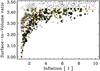 |
Fig. 6 The surface-to-volume ratio for ≈500 valid aggregates (filled symbols) with 81 cubic primary particles, on a cubic grid, normalised to that of the most compact “spherical” structure. The filled symbols are size- and colour-coded as per Fig. 5. The “bare” crosses indicate non-constructable aggregates, as per Fig. 4. |
6.3. Applicability to “real” aggregates?
As interesting as the above results, for the effective cross-sections of aggregates of
cubic grains on a cubic lattice, may appear we really need to consider their relevance to
“real” aggregates consisting of a size distribution of “spheroidal” primary particles.
Firstly, for spheres on the same cubic grid the effective cross-section would be lower by
a factor  when we
take a mean value based upon views exactly along the cartesian axes of the aggregates,
which is a special case that maximises the view of the “pores” between the primary
particles. If we imagine taking the mean values off-set by only a small angle then we
quickly “lose sight of” the pores and approach the value of
⟨σeff⟩ for the array of cubic primary particles. For
spheres on an fcc lattice our derived ⟨σeff⟩ is also
probably a good approximation because, in the fcc lattice where φ = 0.74
(cf. φ = 1 for cubic primary particles) and the maximum coordination
number is 12, there is intrinsically significant shadowing and in projection the “pore
dilution” of ⟨σeff⟩ will be negligible. Similarly, if we
consider pore filling by a mantling “glue” and/or abundant smaller primary particles, then
our “simple cubic cross-section” model probably does a rather good job of estimating the
projected cross-section for an aggregate as a function of D and
I.
when we
take a mean value based upon views exactly along the cartesian axes of the aggregates,
which is a special case that maximises the view of the “pores” between the primary
particles. If we imagine taking the mean values off-set by only a small angle then we
quickly “lose sight of” the pores and approach the value of
⟨σeff⟩ for the array of cubic primary particles. For
spheres on an fcc lattice our derived ⟨σeff⟩ is also
probably a good approximation because, in the fcc lattice where φ = 0.74
(cf. φ = 1 for cubic primary particles) and the maximum coordination
number is 12, there is intrinsically significant shadowing and in projection the “pore
dilution” of ⟨σeff⟩ will be negligible. Similarly, if we
consider pore filling by a mantling “glue” and/or abundant smaller primary particles, then
our “simple cubic cross-section” model probably does a rather good job of estimating the
projected cross-section for an aggregate as a function of D and
I.
This study is not intended to be exhaustive but is meant to be rather indicative and to give some general guidelines for studies of irregular aggregates. Clearly the exact forms of the particles in a study, and therefore their distributions in the D and I space, will depend on the aggregate construction protocol. Nevertheless, the “simple cubic cross-section” model is probably a very good approximation and ought to be widely applicable.
6.4. Implications for gas-grain coupling
In dynamical studies of porous/irregular grains, where gas-grain coupling plays a key role, it is important to have a good measure of the geometrical, or projected, cross-section of the particles. This is particularly so for porous/aggregate dust-gas coupling leading to dust drag/acceleration in circumstellar and disc winds, and in turbulent or shocked gas. Simply “inflating” the grains, using a lowered effective density to model porosity (e.g., Jones et al. 1994) is probably not sufficient because the inflated cross-section is not filled and the surface-to-mass ratio will lower than that predicted by the simple grain-“inflating” approach. In gas-grain coupling studies the projected cross-section for irregular (and “porous”) grains, and the appropriate orientation-averaging, therefore needs to be carefully considered as it will depend upon the adopted aggregate construction protocol.
7. Concluding remarks
We underline the fact that care needs to exercised in the use of the terms porosity and fractal dimension when considering finite-sized interstellar, interplanetary or cometary particles. In detail these grains are not fractal in the true sense of the definition of the term fractal because their structures are not scale-invariant, i.e., a shift in the reference point will not always yield the same fractal dimension.
Often, in coagulation simulations and experiments, the structures appears as rather psuedo-centro-symmetric, in the sense that they appear to have a centre from which extended structures radiate. In contrast, IDP grains are rather “blocky” and do not appear to exhibit “radial”-type structures extending away from a centre.
A new means of characterising the averaged “porosity” and “fractality” of irregular particles is proposed. Given that these two properties of an aggregate are not independent of one another, it seems that may be we should rather think in terms of defining our aggregate, “porous” or “fractal” particles in terms of dimensionality and inflation. A particle’s inflation, I, is a measure of its size compared to the most compact form possible and its dimensionality, D, is a measure of the 3D disposition of the constituent matter in the particle. The parameters I and D can be derived from direct measurements of the particle dimensions (normalised to that of the constituent sub-grains in the case of mono-disperse aggregates). Their usefulness is, in particular, underlined by the fact that I and D can be applied to particles of any arbitrary shape or structure be they solid and homogeneous, have significant concavities and protrusions or consist of porous aggregates of sub-grains or primary particles.
We find that the cross-sections of irregular aggregates can be rather well approximated by simply modelling them as sparse lattices of cubic primary particles on a simple cubic grid and then averaging along the orthogonal x, y and z axes to obtain the mean cross-section.
This study has focussed on aggregates composed of single-sized sub-grains in an attempt to explore their nature and to propose new measures to allow their characterisation. Interstellar grains will in any case be less porous than the rather idealised aggregates considered here because of the effects of ice mantle accretion and the fact that the coagulated grains are formed from a size distribution of primary particles with a clear excess of small over big grains. These factors will tend to lead to pore filling and to aggregates that are more compact and much more strongly bound together due to the extensive surface-to-surface contacts.
A definition of I and D for aggregate particles derived
from a size distribution of primary particles will be rather more complex than the simple
derivations presented but could, in principle, be derived in an analogous way. However, this
may not be necessary because the quantities dimensionality, D, and
inflation, I, can be derived from direct measurements of the particle
dimensions (Li, where
i = x,y or z) and the volume (or
mass) of the constituent solid matter, Vs, i.e.,
(33)and
 (34)
(34)
Acknowledgments
I would like to thank Melanie Köhler and Vincent Guillet for a careful reading of the manuscript and for stimulating discussions on this subject. I would also like to thank the referee for an encouraging review and for useful suggestions. This research was made possible through the key financial support of the Agence National de la Recherche (ANR) through the program Cold Dust (ANR-07-BLAN-0364-01).
References
- Bazell, D., & Dwek, E. 1990, ApJ, 360, 142 [NASA ADS] [CrossRef] [Google Scholar]
- Bohren, C. F., & Huffman, D. R. 1983, Absorption and Scattering of Light by Small Particles (New York: Wiley) [Google Scholar]
- Brown, D. J., Vickers, G. T., Collier, A. P., & Reynolds, G. K. 2005, Chem. Eng. Sci., 60, 289 [CrossRef] [Google Scholar]
- Brownlee, D. E. 1978, in Protostars and Planets: Studies of Star Formation and of the Origin of the Solar System (Tucson: University of Arizona Press), 134 [Google Scholar]
- Bruggemann, D. A. G. 1935, Ann. Phys. (Leipzig), 24, 636 [Google Scholar]
- Dobbins, R. A., & Megaridis, C. M. 1991, Appl. Opt., 30, 4747 [NASA ADS] [CrossRef] [PubMed] [Google Scholar]
- Draine, B. T., & Lee, H. K. 1984, ApJ, 285, 89 [Google Scholar]
- Henning, Th., & Stognienko, R. 1993, A&A, 280, 609 [NASA ADS] [Google Scholar]
- Jones, A. P. 1988, MNRAS, 234, 209 [NASA ADS] [Google Scholar]
- Jones, A. P., Tielens, A. G. G. M., Hollenbach, D. J., & McKee, C. F. 1994, ApJ, 433, 797 [NASA ADS] [CrossRef] [Google Scholar]
- Köhler, M., Guillet, V., & Jones, A. P. 2011, A&A, 528, A96 [NASA ADS] [CrossRef] [EDP Sciences] [Google Scholar]
- Köylü, Ü. Ö., Faeth, G. M., Farais, T. L., & Carvalho, M. G. 1995, Combustion and Flame, 100, 621 [Google Scholar]
- Mackowski, D. W. 2006, JQSRT, 100, 237 [NASA ADS] [CrossRef] [Google Scholar]
- Mackowski, D. W., & Mishchenko, M. I. 1996, J. Opt. Soc. Am. A, 13, 2266 [NASA ADS] [CrossRef] [Google Scholar]
- Mandelbrot, B. B. 1982, The Fractal Geometry of Nature (San Francisco: Freeman) [Google Scholar]
- Mathis, J. S., & Whiffen, G. 1989, ApJ, 341, 808 [NASA ADS] [CrossRef] [Google Scholar]
- Micelotta, E. R., Jones, A. P., & Tielens, A. G. G. M. 2010, A&A, 510, A36 [NASA ADS] [CrossRef] [EDP Sciences] [Google Scholar]
- Min, M., Hovenier, J. W., & de Koter, A. 2005, A&A, 432, 909 [NASA ADS] [CrossRef] [EDP Sciences] [Google Scholar]
- Min, M., Dominik, C., Hovenier, J. W., de Koter, A., & Waters, L. B. F. M. 2006a, A&A, 445, 1005 [NASA ADS] [CrossRef] [EDP Sciences] [MathSciNet] [Google Scholar]
- Min, M., Hovenier, J. W., Dominik, C., de Koter, A., & Yurkin, M. A. 2006b, J. Quant. Spectrosc. Radiat. Transfer, 97, 161 [Google Scholar]
- Muinonen, K. 1996, J. Quant. Spectrosc. Radiat. Transfer, 55, 603 [NASA ADS] [CrossRef] [Google Scholar]
- Muinonen, K., Nousiannen, T., Fast, P., Lumme, K., & Peltoniemi, J. I. 1996, J. Quant. Spectrosc. Radiat. Transfer, 55, 577 [Google Scholar]
- Mutschke, H., Min, M., & Tamanai, A. 2009, A&A, 504, 875 [NASA ADS] [CrossRef] [EDP Sciences] [Google Scholar]
- Ormel, C. W., Spaans, M., & Tielens, A. G. G. M. 2007, A&A, 461, 215 [NASA ADS] [CrossRef] [EDP Sciences] [Google Scholar]
- Ormel, C. W., Paszun, D., Dominik, C., & Tielens, A. G. G. M. 2009, A&A, 502, 845 [NASA ADS] [CrossRef] [EDP Sciences] [Google Scholar]
- Ossenkopf, V. 1993, A&A, 280, 617 [NASA ADS] [Google Scholar]
- Perrin, J.-M., & Sivan, J.-P. 1990, A&A, 228, 238 [NASA ADS] [Google Scholar]
- Perrin, J.-M., & Sivan, J.-P. 1991, A&A, 247, 497 [NASA ADS] [Google Scholar]
- Rietmeijer, F. 1998, in Rev. Min., ed. J. Papike (Washington, DC: The Mineralogical Society of America), 36, 21295 [Google Scholar]
- Rouleau, F., & Martin, P. G. 1991, ApJ, 377, 526 [NASA ADS] [CrossRef] [Google Scholar]
- Shen, Y., Draine, B. T., & Johnson, E. T. 2008, ApJ, 689, 260 [NASA ADS] [CrossRef] [Google Scholar]
- Shen, Y., Draine, B. T., & Johnson, E. T. 2009, ApJ, 696, 2126 [NASA ADS] [CrossRef] [Google Scholar]
- Skorov, Yu. V., Keller, H. U., & Rodin, A. V. 2010, P&SS, 58, 1802 [NASA ADS] [Google Scholar]
- Stauffer, D., & Aharony, A. 1994, Introduction to Percolation Theory, 2nd Ed. (Boca Raton, Florida: CRC Press) [Google Scholar]
- Voshchinnikov, N. V., Il’in, V. B., & Henning, Th. 2005, A&A, 429, 371 [NASA ADS] [CrossRef] [EDP Sciences] [Google Scholar]
- Wolff, M. J., Clayton, G. C., Martin, P. G., & Schulte-Ladbeck, R. E. 1994, ApJ, 423, 412 [NASA ADS] [CrossRef] [Google Scholar]
- Wolff, M. J., Clayton, G. C., & Gibson, S. J. 1998, ApJ, 503, 814 [Google Scholar]
- Xu, Y. 1995, Appl. Opt., 34, 4573 [NASA ADS] [CrossRef] [PubMed] [Google Scholar]
Appendix A: Extended particle properties
With the interpretation of the interstellar dust emission observations from the Herschel and Planck missions very much in mind, we are obviously interested in the long wavelength emission from dust and dust aggregates, and therefore in the absorption cross-section, which is equal to the emission cross-section, Cabs = Cem. In the following we explore the cross-sectional properties of aggregates of sub-grains.
A.1. Orientation-averaged cross-sections
The orientation-averaged cross-section factor, ⟨S⟩, (the effective
cross-section normalised to the maximum cross-section) for a particle is obviously
⟨S⟩ = 1 for a sphere (all particle axes equal). For a thin disc
Micelotta et al. (2010) find
 . For a
randomly-tumbling cylinder Brown et al. (2005)
show that the effective cross-section is
. For a
randomly-tumbling cylinder Brown et al. (2005)
show that the effective cross-section is  , where r
is the cylinder radius and l is its length, which corresponds to:
, where r
is the cylinder radius and l is its length, which corresponds to:
 (A.1)If we take the
particle enclosing volume, Ve, normalised to the
sub-particle size d, to be
Ve/d3 = π (Nx Ny Nz)/6
(see Eq. (14)), then the sub-particle
size-normalised, orientation-averaged, “enclosing” particle cross-section is given by:
(A.1)If we take the
particle enclosing volume, Ve, normalised to the
sub-particle size d, to be
Ve/d3 = π (Nx Ny Nz)/6
(see Eq. (14)), then the sub-particle
size-normalised, orientation-averaged, “enclosing” particle cross-section is given by:
 (A.2)which is not
filled, except for compact particles. However, we need to determine the actual
geometrical cross-section of the extended, porous particle (the fraction of the
cross-section σe that is filled), i.e., the total projected
cross-section, or the geometrical filling factor of Ormel et al. (2009). Unfortunately, Ormel et
al. (2009) and (2007) give no indication
as to how the geometrical filling factors and enlargement parameters were actually
calculated for their particles.
(A.2)which is not
filled, except for compact particles. However, we need to determine the actual
geometrical cross-section of the extended, porous particle (the fraction of the
cross-section σe that is filled), i.e., the total projected
cross-section, or the geometrical filling factor of Ormel et al. (2009). Unfortunately, Ormel et
al. (2009) and (2007) give no indication
as to how the geometrical filling factors and enlargement parameters were actually
calculated for their particles.
This problem was studied by Köylü et al. (1995),
based on earlier work cited therein, within the context of soot particle aggregate
structures. They found that, for agglomerated soot particles with a fractal dimension
Df ~ 1.8, the number of primary particles,
N, within the aggregate can be expressed as:  (A.3)where
ka is constant close to unity,
Aa is projected area of the aggregate and
Ap is the cross-section of a primary particle,
π(d/2)2. Köylü et al. (1995) considered aggregates of primary
particles or sub-grains. A power-law correlation is found to give an excellent fit to
their data with ka = 1.15 ± 0.02 and an index
α = 1.10 ± 0.004. The experimental uncertainty in
α is apparently very small (see Fig. A.1) and we will therefore subsequently ignore it. Thus, the projected area,
or effective cross-section, ⟨σeff⟩, of their fractal
particles is given by
(A.3)where
ka is constant close to unity,
Aa is projected area of the aggregate and
Ap is the cross-section of a primary particle,
π(d/2)2. Köylü et al. (1995) considered aggregates of primary
particles or sub-grains. A power-law correlation is found to give an excellent fit to
their data with ka = 1.15 ± 0.02 and an index
α = 1.10 ± 0.004. The experimental uncertainty in
α is apparently very small (see Fig. A.1) and we will therefore subsequently ignore it. Thus, the projected area,
or effective cross-section, ⟨σeff⟩, of their fractal
particles is given by 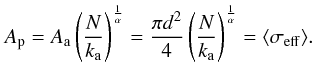 (A.4)As noted above this
appears to be valid for a limited range of fractal dimension applicable to soot
aggregate particles (Df ≈ 1.7−1.9). The above expression
can be more generally expressed as:
(A.4)As noted above this
appears to be valid for a limited range of fractal dimension applicable to soot
aggregate particles (Df ≈ 1.7−1.9). The above expression
can be more generally expressed as:
 (A.5)For an extended,
rod-like aggregate (Df = 1), where most, if not all, of the
primary particles are “visible”, we have
⟨σeff⟩ = (N πd2)/4
(i.e., c = 1 and β = 1), and for the case of the most
compact spherical aggregate (Df = 3) of primary particles it
can be shown that
(A.5)For an extended,
rod-like aggregate (Df = 1), where most, if not all, of the
primary particles are “visible”, we have
⟨σeff⟩ = (N πd2)/4
(i.e., c = 1 and β = 1), and for the case of the most
compact spherical aggregate (Df = 3) of primary particles it
can be shown that  (i.e., c = 1 and
  ).
Figure A.1 shows these three determined values
for α as a function of Df along with an
analytical fit to these data (
).
Figure A.1 shows these three determined values
for α as a function of Df along with an
analytical fit to these data ( ). Here,
and in the absence of evidence to the contrary, we make the (probably incorrect)
assumption that ka is indepdent of
Df over the entire range of
Df. The use of Eq. (A.4), and the dependence of α on
Df, now enables us to calculate the projected
cross-section for any collection of primary particles of a given fractal dimension or
fractality, i.e.,
). Here,
and in the absence of evidence to the contrary, we make the (probably incorrect)
assumption that ka is indepdent of
Df over the entire range of
Df. The use of Eq. (A.4), and the dependence of α on
Df, now enables us to calculate the projected
cross-section for any collection of primary particles of a given fractal dimension or
fractality, i.e., 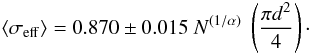 (A.6)This expression
is plotted in Fig. A.2, as the normalised function
⟨σeff⟩/((Nπd2)/4),
for aggregates with 10–1000 primary particles. What this figure shows is that for highly
fractal particles (Df = 1) the effective cross-section,
⟨σeff⟩, scales directly with the number of the primary
particles, N, and their cross-section,
π(d/2)2. This shows
that for Df = 1 the angle-averaged cross-section is only 87%
of the total cross-section of all the constituent sub-grains, i.e.,
Nπ(d/2)2, which
implies that some of the primary particles are “shadowed” in the orientation-averaged
projection as clearly must be the case. For a randomly tumbling cylinder
(Df ~ 1) setting ⟨S⟩ = 0.87 in
Eq. (A.1) corresponds to a cylinder
with l ≈ 10r.
(A.6)This expression
is plotted in Fig. A.2, as the normalised function
⟨σeff⟩/((Nπd2)/4),
for aggregates with 10–1000 primary particles. What this figure shows is that for highly
fractal particles (Df = 1) the effective cross-section,
⟨σeff⟩, scales directly with the number of the primary
particles, N, and their cross-section,
π(d/2)2. This shows
that for Df = 1 the angle-averaged cross-section is only 87%
of the total cross-section of all the constituent sub-grains, i.e.,
Nπ(d/2)2, which
implies that some of the primary particles are “shadowed” in the orientation-averaged
projection as clearly must be the case. For a randomly tumbling cylinder
(Df ~ 1) setting ⟨S⟩ = 0.87 in
Eq. (A.1) corresponds to a cylinder
with l ≈ 10r.
As the particle fractality (and hence the “porosity”) increase Fig. A.2 shows that the normalised effective cross-section decreases rapidly with N as the number of primary particles that are “hidden” within the structure increases. This is simply the effect of decreasing surface-to-volume ratio as the size, or number of primary particles, increases. For typical soot, cluster-cluster aggregates with Df ~ 1.7−1.9 it can be seen that the normalised cross-section is ≈40–80% of the total primary particle cross-section (Nπ(d/2)2).
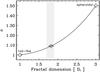 |
Fig. A.1 Aggregate projected area exponent, α, versus fractal dimension, Df, or equivalently the dimensionality, D. The data point at Df = 1.82 (with the uncertainties in Df and α indicated by the horizontal and vertical bars) is the best-fit value of α for soot aggregates, which have 1.7 ≤ Df ≤ 1.9 (shaded range), taken from Köylü et al. (1995). |
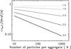 |
Fig. A.2 The normalised projected cross-section, ⟨σeff⟩/((Nπd2)/4), for aggregates consisting of 10–1000 primary particles of given fractal dimension or fractality (indicated by the number at right). The experimental uncertainties are of about the same order as the thickness of the Df = 3 line. |
A.2. Extended particle radii of gyration
As pointed out by Mandelbrot (1982); Dobbins & Megaridis (1991); Ossenkopf (1993), Köylü et al. (1995) and Mackowski
(2006), in aggregated particle studies a quantity of prime importance for the
optical and collisional properties of the particles is the radius of gyration,
Rg, which in these works is defined as:
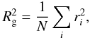 (A.7)where
ri is the distance of the individual
primary particle from the centre of mass of the aggregate. The soot particle and
simulation studies by Köylü et al. (1995) further
indicate that
(A.7)where
ri is the distance of the individual
primary particle from the centre of mass of the aggregate. The soot particle and
simulation studies by Köylü et al. (1995) further
indicate that 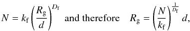 (A.8)where, from
experiment, Df = 1.82 ± 0.08 and
kf = 8.5 ± 0.5.
(A.8)where, from
experiment, Df = 1.82 ± 0.08 and
kf = 8.5 ± 0.5.
Mackowski (2006) in a similar study, but based
only on simulations (references therein), find that
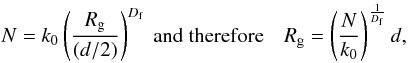 (A.9)and that the variation
of the factor k0 with Df can be
expressed as
k0 = (1.27−2.2[Df − 1.82]).
We can see that the two k factors above are simply related by
k0 = (1/2)Dfkf.
Upon substitution it can be shown that there is an apparent discrepancy between the
experimental and simulation fits, in that
kf/k0 = 1.9
at Df = 1.82. Nevertheless, we can use the above expressions
for k0(Df) to derive an
equivalent fractal dependence for
kf(Df), i.e.,
kf = 8.5(2.82 − Df), which
obviously reduces to the above value of kf = 8.5 when
Df = 1.82.
(A.9)and that the variation
of the factor k0 with Df can be
expressed as
k0 = (1.27−2.2[Df − 1.82]).
We can see that the two k factors above are simply related by
k0 = (1/2)Dfkf.
Upon substitution it can be shown that there is an apparent discrepancy between the
experimental and simulation fits, in that
kf/k0 = 1.9
at Df = 1.82. Nevertheless, we can use the above expressions
for k0(Df) to derive an
equivalent fractal dependence for
kf(Df), i.e.,
kf = 8.5(2.82 − Df), which
obviously reduces to the above value of kf = 8.5 when
Df = 1.82.
In these studies another characteristic, or rather characterising, parameter is the
longest particle dimension, the maximum projected length L, which is
simply related to the above-used quantity,
NL + (see Sect. 5.2), by
L = NL + × d.
Köylü et al. (1995) give the following useful
relationship: 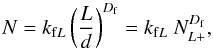 (A.10)which, when the
constant kfL is known, can be used to
derive the fractal dimension of a particle from measurements of its number of
constituent primary particles, its maximum projected length and the size of the primary
particles, i.e.,
Df = (log N − log kfL)/log NL + .
(A.10)which, when the
constant kfL is known, can be used to
derive the fractal dimension of a particle from measurements of its number of
constituent primary particles, its maximum projected length and the size of the primary
particles, i.e.,
Df = (log N − log kfL)/log NL + .
Using the above equations that express N as a function of
Aa (Eq. (A.3)) and of Rg (Eq. (A.8)), and substituting, we obtain the
following relationshipfor Rg as a function
Aa,
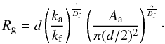 (A.11)This is useful because
it allows us to calculate the radius of gyration, Rg, of an
aggregate from known quantities and the calculated projected cross-section of the
particle (Eq. (A.3)). However, its
utility does depend on knowing, or assuming, values for the parameters
ka and kf.
(A.11)This is useful because
it allows us to calculate the radius of gyration, Rg, of an
aggregate from known quantities and the calculated projected cross-section of the
particle (Eq. (A.3)). However, its
utility does depend on knowing, or assuming, values for the parameters
ka and kf.
A.3. Extended particle optical properties
The optical properties of soot aggregates (with Df ~ 1.8)
have been studied by Dobbins & Megaridis
(1991) who derive the angle- and distribution-averaged absorption and
scattering properties. Dobbins & Megaridis
(1991) find that the absorption cross-section for polydisperse, fractal-like
aggregates with Df = 1.7−1.9 is:
 (A.12)where,
according to their definitions,
(A.12)where,
according to their definitions,  is
the average number of primary particles per aggregate, N (the first
moment of their aggregate size probability function,
p(N)),
xp = (πd)/λ ≪ 1,
E(m) = −Im[(m2 − 1)/(m2 + 2)]
and k = (2π)/λ.
With the, partial, substitution for the primary particle radius
d = 2a and some re-arrangement it can be shown that,
with x = (2πa)/λ,
the above absorption cross-section is simply, in the more usual nomenclature,
is
the average number of primary particles per aggregate, N (the first
moment of their aggregate size probability function,
p(N)),
xp = (πd)/λ ≪ 1,
E(m) = −Im[(m2 − 1)/(m2 + 2)]
and k = (2π)/λ.
With the, partial, substitution for the primary particle radius
d = 2a and some re-arrangement it can be shown that,
with x = (2πa)/λ,
the above absorption cross-section is simply, in the more usual nomenclature,
![Mathematical equation: \appendix \setcounter{section}{1} \begin{eqnarray} {\bar C_{\rm abs}^A} &=& N \pi d^2 \times \frac{2 \pi a}{\lambda} \left\{ - {\rm Im} \left[ \frac{m^2-1}{m^2+2} \right] \right\} \nonumber\\ & =& \frac{N \pi d^2}{4} \times 4 x \left\{ - {\rm Im} \left[ \frac{m^2-1}{m^2+2} \right] \right\} \end{eqnarray}](/articles/aa/full_html/2011/04/aa15968-10/aa15968-10-eq327.png) (A.13)which
is just the total geometrical cross-section of the primary particles,
Nπ(d/2)2, multiplied
by the absorption cross-section for a single primary particle in the Rayleigh limit. The
angle-averaged scattering cross-section derived by Dobbins & Megaridis (1991) is more complex, involving the second
moment of their aggregate size probability function,
p(N), but for the purposes of the long-wavelength
emission from aggregates does not concern us here. This approximation, via the
Rayleigh-Gans (RG) theory, is often used in the context of soot particle studies.
(A.13)which
is just the total geometrical cross-section of the primary particles,
Nπ(d/2)2, multiplied
by the absorption cross-section for a single primary particle in the Rayleigh limit. The
angle-averaged scattering cross-section derived by Dobbins & Megaridis (1991) is more complex, involving the second
moment of their aggregate size probability function,
p(N), but for the purposes of the long-wavelength
emission from aggregates does not concern us here. This approximation, via the
Rayleigh-Gans (RG) theory, is often used in the context of soot particle studies.
As pointed out by Mackowski (2006), the RG approximation, in the Rayleigh-limit, generally under predicts the absorption cross-sections of aggregates of spheres that have refractive indices typical of carbonaceous soots. Mackowski (2006) undertook a detailed theoretical/simulation study of the effects of aggregation on the optical properties of soot particles and arrived an elegant and simple model for predicting their absorption in relation to the properties predicted by the RG model. In essence, Mackowski finds that, for large aggregates (N ≥ 100), the RG model results underpredict the relevant cross-sections by as much as a factor of two but that this discrepancy strongly depends on the value of the complex refractive index at the wavelength of interest. For soot aggregates the RG model underestimate is found to be of the order of 10% at visible wavelengths and a factor of two in the mid-infrared. The reader is recommended to take a close look at the work by Mackowski (2006) for further details of the proposed simple model methodology.
The optical properties of irregular particles have also been dealt with using a Gaussian random particle approach (Muinonen 1996; Muinonen et al. 1996) and a distribution of form factors (DFF) based on the gaussian random particle approach (Min et al. 2006a,b; Mutschke et al. 2009). With these models it is possible to calculate the absorption and scattering of highly irregular particles.
Köhler et al. (2011) have studied the effects of refractive index, particle-particle contact and grain mantling on the emissivity of coagulated particles within the astrophysical context. They find that the grain-grain contact surfaces introduced in the discrete dipole approximation (DDA) model for coagulated grains can, depending on the material properties, explain the observed enhancement in the particle emissivity at far-infrared and sub-mm wavelengths.
Appendix B: Multi-component effective media
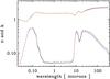 |
Fig. B.1 A comparison of the three-component Bruggemann EMT-generated n (upper curves) and k (lower curves) data for a mix of a-Sil (0.4), a-C:H (0.2) and vacuum (0.4) by volume (orange dashed line), with pair-wise mixing using the Bruggemann EMT. The pair-wise mixing order [(1+2)i+3m] is: [(a-Sil+a-C:H)+vac] and [(a-C:H+a-Sil)+vac] – green lines, [(a-Sil+vac)+a-C:H] and [(vac+a-Sil)+a-C:H] – upper blue lines, [(a-C:H+vac)+a-Sil] and [(vac+a-C:H)+a-Sil] – lower blue lines. |
In the Bruggemann effective medium theory (EMT) the effective dielectric function,
ϵav, of a fractional volume of inclusions,
fi, of dielectric function ϵi in
a matrix of of dielectric function ϵm is found from the
equation (Bruggemann 1935) ![Mathematical equation: \appendix \setcounter{section}{2} \begin{equation} f_{\rm i} \left[ \frac{\epsilon_{\rm i} - \epsilon_{\rm av}}{\epsilon_{\rm i} + 2 \epsilon_{\rm av}} \right] + (1-f_{\rm i}) \left[ \frac{\epsilon_{\rm m} - \epsilon_{\rm av}}{\epsilon_{\rm m} + 2 \epsilon_{\rm av}} \right] = 0. \label{eq_BEMT} \end{equation}](/articles/aa/full_html/2011/04/aa15968-10/aa15968-10-eq337.png) (B.1)For a binary mix
this involves solving a quadratic equation, for three components a cubic equation etc. In
Fig. B.1 we compare the mixing of the Draine & Lee (1984) astronomical silicate
(a-Sil), Rouleau & Martin (1991) BE
amorphous carbon (a-C:H) and vacuum components, obtained using the Bruggemann rule for
three components, with a pair-wise mixing of the same three components in the same volume
fractions. In this pair-wise mixing scheme components 1i
(inclusion) and 2m (matrix) are first mixed and then the “effective” result of
this pair mixed with a third component, i.e.,
[(1 + 2)i + 3m]. We note that in the
pair-wise mixing case the results are not commutative, except for the case of switching
inclusions and matrix in the first pair-wise effective medium calculation. We find that
where the mixing is performed in the order of most refractive to least refractive, i.e.,
silicate → carbon → ice → vacuum, the pair-wise method gives an excellent match to
n and k in comparison with the exact three-component
Bruggemann calculation, except for the lowest values of k at mid-infrared
wavelengths (see Fig. B.1).
(B.1)For a binary mix
this involves solving a quadratic equation, for three components a cubic equation etc. In
Fig. B.1 we compare the mixing of the Draine & Lee (1984) astronomical silicate
(a-Sil), Rouleau & Martin (1991) BE
amorphous carbon (a-C:H) and vacuum components, obtained using the Bruggemann rule for
three components, with a pair-wise mixing of the same three components in the same volume
fractions. In this pair-wise mixing scheme components 1i
(inclusion) and 2m (matrix) are first mixed and then the “effective” result of
this pair mixed with a third component, i.e.,
[(1 + 2)i + 3m]. We note that in the
pair-wise mixing case the results are not commutative, except for the case of switching
inclusions and matrix in the first pair-wise effective medium calculation. We find that
where the mixing is performed in the order of most refractive to least refractive, i.e.,
silicate → carbon → ice → vacuum, the pair-wise method gives an excellent match to
n and k in comparison with the exact three-component
Bruggemann calculation, except for the lowest values of k at mid-infrared
wavelengths (see Fig. B.1).
In the absence of having solved the quartic, and higher equations, for four and more component mixes we postulate that this pairwise calculation of an effective medium using the Bruggemann mixing rule can be used to calculate the effective medium of any number of mixed media, provided that the materials are mixed in the order of most to least refractory. Thus, this method (the pair-wise Bruggemann EMT or PWB-EMT) can be used to limit the complexity of the calculation of multi-material effective media to the solution of quadratic equations. For example, this method could facilitate studies of inhomogeneous, irregular and “porous” aggregates consisting of amorphous silicates and amorphous carbons with ice mantles, i.e., a four-component mix, without having to solve the quartic version of Eq. (B.1).
Appendix C: Cabs at long wavelengths for n constant
At long wavelengths the absorption (and emission) cross-section of a particle of radius
a is given by ![Mathematical equation: \appendix \setcounter{section}{3} \begin{equation} C_{\rm abs} = 4 x \ \left\{ - {\rm Im} \left[ \frac{m^2-1}{m^2+2} \right] \right\} \ \pi a^2. \label{eq_Cabs_1} \end{equation}](/articles/aa/full_html/2011/04/aa15968-10/aa15968-10-eq346.png) (C.1)Substituting
x = 2πaeff/λ,
where aeff is the effective radius of the solid matter in the
aggregate/particle, and m = n − ik for
the complex index of refraction, and solving for the imaginary part of the refractive
index term we have
(C.1)Substituting
x = 2πaeff/λ,
where aeff is the effective radius of the solid matter in the
aggregate/particle, and m = n − ik for
the complex index of refraction, and solving for the imaginary part of the refractive
index term we have 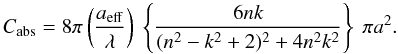 (C.2)For astronomical silicate
grains (Draine & Lee 1984) at wavelengths
longer than 100 μm n is constant and
n > k
(n ≃ 3.4, k ≲ 0.5, see Fig. C.1, i.e., n2 ≃ 11.6,
k2 ≲ 0.25 and
n2k2 ≲ 2.9). Neglecting the
k2 terms the above yields a simple expression for the
absorption cross-section for solid and “porous” Draine
& Lee (1984) astronomical silicate grains, i.e.,
(C.2)For astronomical silicate
grains (Draine & Lee 1984) at wavelengths
longer than 100 μm n is constant and
n > k
(n ≃ 3.4, k ≲ 0.5, see Fig. C.1, i.e., n2 ≃ 11.6,
k2 ≲ 0.25 and
n2k2 ≲ 2.9). Neglecting the
k2 terms the above yields a simple expression for the
absorption cross-section for solid and “porous” Draine
& Lee (1984) astronomical silicate grains, i.e.,
![Mathematical equation: \appendix \setcounter{section}{3} $$ C_{\rm abs} = 8 \pi \left( \frac{a_{\rm eff}} {\lambda\ (1-f_{\rm v})^{\frac{1}{3}}} \right) \left[ \frac{6n}{(n^2+2)^2} \right] \bigg\{ k_{\rm solid} \bigg\} \ \pi a^2 $$](/articles/aa/full_html/2011/04/aa15968-10/aa15968-10-eq360.png)
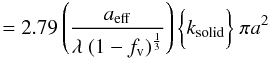 (C.3)where
ksolid is the imaginary part of the complex index of
refraction of the solid material at wavelength λ and
fv is the volume fraction of vacuum in the particle. Note
that a is the outer radius of the “inflated” porous particle and
aeff is the effective radius for the solid matter within the
particle. For non-porous particles a = aeff.
The above approximation to Cabs is equivalent to a simple
dilution of the absorptive index, ksolid, of the solid
material by a factor
(a/aeff)3.
(C.3)where
ksolid is the imaginary part of the complex index of
refraction of the solid material at wavelength λ and
fv is the volume fraction of vacuum in the particle. Note
that a is the outer radius of the “inflated” porous particle and
aeff is the effective radius for the solid matter within the
particle. For non-porous particles a = aeff.
The above approximation to Cabs is equivalent to a simple
dilution of the absorptive index, ksolid, of the solid
material by a factor
(a/aeff)3.
In Fig. C.2 we show this fit, together with that calculated using the Mie theory (and the Bruggemann EMT where there is a vacuum component). We find that this approximation can reproduce Cabs to within ± 6% for porosities ≲50%. This analytical approximation is only valid at long wavelengths (e.g., the far-infrared and longward) and for materials where n is constant. For amorphous carbons in general n is not constant at long wavelengths and this very simple approximation will not work for these materials.
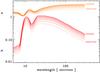 |
Fig. C.1 n (upper) and k (lower) for astronomical silicate particles with 0, 10, 20, 30, 40 an 50% vaccuum (line thickness decreases with increasing vacuum fraction) calculated using the Bruggemann EMT. |
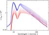 |
Fig. C.2 The absorption cross-section, multiplied by the wavelength for clarity, for astronomical silicate particles with 0, 10, 20, 30, 40 an 50% vaccuum (line thickness decreases with increasing vacuum fraction), and effective radii 100, 104, 108, 113, 119 and 126 nm, respectively, calculated using Mie theory and the Bruggemann EMT (blue lines). The red lines show the simple analytical fits (see text). |
This surprisingly-simple approach shows that we need not resort to the Mie theory nor an EMT-averaging to calculate the the dust cross-sections for solid or porous grains at long wavelengths where n is constant. However, its usefulness needs to be tested against laboratory data for real interstellar dust analogue materials at long wavelengths.
All Tables
The dimensionality, D, and inflation, I, for regular geometrical solids. a and l are the relevant radius and side/edge lengths, respectively.
All Figures
|
Fig. 1 Axis sum, Σi, vs. axis product, Πi, plot for a particle containing 100 identical sub-particles as a function of the dimensionality (as indicated): D = 1 (diamond), 1.5 (plus signs), 2 (triangles), 2.5 (crosses) and 3 (squares). Compact particles are to the lower left and extended particles to the upper right. Note that no porosity is allowed for D = 1, rod-like particles. |
| In the text | |
|
Fig. 2 Dimensionality, D, versus inflation, I, plot for particles containing 50 equal-sized constituents for ≈15 000 randomly-generated structures (with φ = 1). The inset box shows the limits on D (1 ≤ D ≤ 3) and I (1 ≤ I ≤ N2/27), and the middle vertical line shows the limit for an idealised 2D particle, i.e., I = N/4. |
| In the text | |
|
Fig. 3 Same as for Fig. 2 except that we have now volume- and shape-weighted the data point sizes by a factor (1 − [D − 2]2)/I (see text). |
| In the text | |
|
Fig. 4 The same as Fig. 3 but for ≈500 aggregates
(consisting of 81 cubic primary particles) and a more limited range of
I (≤10). The symbols (filled circles) are size-scaled by
|
| In the text | |
|
Fig. 5 The effective cross-section, normalised to the number of primary particles, N, for ≈500 aggregates constructed from 81 cubic primary particles on a cubic grid. The symbols (black filled circles and coloured plus signs) are size-scaled by the particle dimensionality, D. The plus signs colour-code (see key at bottom right of the figure) the binned dimensionality (red D = 1–1.5; yellow D = 1.5–2; green D = 2–2.5; blue D = 2.5–2). The orange lines shows some representative analytical fits (see text). |
| In the text | |
|
Fig. 6 The surface-to-volume ratio for ≈500 valid aggregates (filled symbols) with 81 cubic primary particles, on a cubic grid, normalised to that of the most compact “spherical” structure. The filled symbols are size- and colour-coded as per Fig. 5. The “bare” crosses indicate non-constructable aggregates, as per Fig. 4. |
| In the text | |
|
Fig. A.1 Aggregate projected area exponent, α, versus fractal dimension, Df, or equivalently the dimensionality, D. The data point at Df = 1.82 (with the uncertainties in Df and α indicated by the horizontal and vertical bars) is the best-fit value of α for soot aggregates, which have 1.7 ≤ Df ≤ 1.9 (shaded range), taken from Köylü et al. (1995). |
| In the text | |
|
Fig. A.2 The normalised projected cross-section, ⟨σeff⟩/((Nπd2)/4), for aggregates consisting of 10–1000 primary particles of given fractal dimension or fractality (indicated by the number at right). The experimental uncertainties are of about the same order as the thickness of the Df = 3 line. |
| In the text | |
|
Fig. B.1 A comparison of the three-component Bruggemann EMT-generated n (upper curves) and k (lower curves) data for a mix of a-Sil (0.4), a-C:H (0.2) and vacuum (0.4) by volume (orange dashed line), with pair-wise mixing using the Bruggemann EMT. The pair-wise mixing order [(1+2)i+3m] is: [(a-Sil+a-C:H)+vac] and [(a-C:H+a-Sil)+vac] – green lines, [(a-Sil+vac)+a-C:H] and [(vac+a-Sil)+a-C:H] – upper blue lines, [(a-C:H+vac)+a-Sil] and [(vac+a-C:H)+a-Sil] – lower blue lines. |
| In the text | |
|
Fig. C.1 n (upper) and k (lower) for astronomical silicate particles with 0, 10, 20, 30, 40 an 50% vaccuum (line thickness decreases with increasing vacuum fraction) calculated using the Bruggemann EMT. |
| In the text | |
|
Fig. C.2 The absorption cross-section, multiplied by the wavelength for clarity, for astronomical silicate particles with 0, 10, 20, 30, 40 an 50% vaccuum (line thickness decreases with increasing vacuum fraction), and effective radii 100, 104, 108, 113, 119 and 126 nm, respectively, calculated using Mie theory and the Bruggemann EMT (blue lines). The red lines show the simple analytical fits (see text). |
| In the text | |
Current usage metrics show cumulative count of Article Views (full-text article views including HTML views, PDF and ePub downloads, according to the available data) and Abstracts Views on Vision4Press platform.
Data correspond to usage on the plateform after 2015. The current usage metrics is available 48-96 hours after online publication and is updated daily on week days.
Initial download of the metrics may take a while.