| Issue |
A&A
Volume 527, March 2011
|
|
|---|---|---|
| Article Number | A12 | |
| Number of page(s) | 8 | |
| Section | The Sun | |
| DOI | https://doi.org/10.1051/0004-6361/201016075 | |
| Published online | 19 January 2011 | |
Magnetoacoustic surface gravity waves at a spherical interface
1
Solar Physics and Space Plasma Research Centre
(SP 2RC), Dept. of Applied Mathematics,
University of Sheffield,
Hicks Building, Hounsfield Road,
Sheffield
S3 7RH,
UK
e-mail: i.ballai@sheffield.ac.uk
2
Eötvös University, Department of Astronomy,
1117 Budapest, 1/A Pázmány Péter,
Budapest,
Hungary
Received:
4
November
2010
Accepted:
20
December
2010
Aims. The plasma structured by magnetic fields in the solar atmosphere is a perfect medium for the propagation of guided magnetic and magnetoacoustic waves. Geometrical restriction of wave propagation is known to confer a dispersive character for waves. In addition, waves propagating along discontinuities in the medium are known to remain localized. As an extension to theories of guided waves in magnetic slabs and cylinders under solar and stellar conditions, we aim to study the propagation of magnetoacoustic-gravity waves at a spherical interface in the low solar corona (considered here as a density discontinuity), modelling global waves recently observed in the corona in EUV wavelengths.
Methods. Using conservation laws at the interface we derive the dispersion relation in spherical geometry with a radially expanding magnetic field in the presence of gravitational stratification. The obtained dispersion relation describing fast magnetoacoustic-gravity surface waves is derived using an approximative method taking into account that propagation takes place near the solar surface.
Results. Theoretical results obtained in the present study are applied to investigate the propagation of EIT waves in the low corona. The frequency of waves is shown to increase with decreasing density contrast at the interface. We also show that, for a given azimuthal wavenumber, the magnetic field has a very small effect on the value of the frequency of waves. When plotted against the location of the interface (in the radial direction) the frequency varies inversely proportional to the distance, while for a fixed density ratio and location of the interface the frequency is obtained to be defined in a very narrow region.
Key words: magnetohydrodynamics (MHD) / Sun: corona / waves
© ESO, 2011
1. Introduction
The magnetic field in the solar atmosphere tends to accumulate in various entities such as sunspots, pores, spiculae, coronal loops, plumes, etc. The idea that separated magnetic structures can act as channels for wave propagation was recognised a long time ago (see, e.g. Wilson 1980; Roberts 1981a,b; Edwin & Roberts 1983; Roberts et al. 1984; Cally 1986). Stresses created in the convective zone could travel in the form of, e.g. waves, some of them being able to reach even the solar corona. Numerous pieces of evidence for waves in various solar structures have been adduced since high resolution space satellite observation became available. Theoretical models on wave propagation in structured plasmas (e.g. Roberts 1981a,b; Edwin & Roberts 1983; Roberts et al. 1984) were developed within the framework of magnetohydrodynamics (MHD) at a time when observations were sporadic and mainly in the radio-frequency domain (see, e.g. Kai & Takayanagi 1973; Aschwanden et al. 1991). Nowadays theoretical predictions are continuously confirmed by high-resolution observations in (extreme) ultraviolet (for excellent reviews on solar atmospheric waves see, e.g. Nakariakov & Verwichte 2005; Banerjee et al. 2007, and references therein).
With the advent of high resolution observations, coronal seismology emerged as one of the newest branches of modern solar physics, where advances are achieved in diagnosing the structure, the magnitude and sub-resolution structure of the magnetic fields, densities, scale heights, heating functions, etc. (Nakariakov et al. 1999; Ballai 2007; Ruderman et al. 2008) with the help of observable properties of waves and oscillations.
In the theory of MHD waves special attention has been paid to guided waves propagating in various magnetic structures. As a result of propagation in geometrically restricted magnetic “channels”, waves become dispersive with their dispersion relation given in terms of hyperbolic/trigonometric functions for magnetic slabs (Roberts 1981b) and Bessel functions in magnetic cylinders (Edwin & Roberts 1983). Mathematically tractable forms for dispersion relations were obtained in the long wavelength (i.e. for wavelengths much longer than the transversal geometrical size of the waveguide) and short wavelength limits. In general most previous studies considered that the magnetic field is along the density interface. In connection with prominence oscillations Joarder & Roberts (1992) and Oliver et al. (1993) determined the propagation characteristics of waves when the magnetic field was perpendicular (or inclined) to the density jump.
Although significant advances in the theory of guided MHD waves were achieved for waves propagating in a magnetic slab (i.e. Cartesian geometry) and magnetic flux tubes (i.e. cylindrical geometry), very little is known on the properties of guided waves in spherical geometry. The very low number of studies on waves in spherical geometry (compared with other geometries) could be attributed to the fact that for a long time no spherical large scale waves were observed, but also to the mathematical description of wave propagation in this geometry being rather cumbersome. Neglecting the magnetic field, the hydrodynamical approach of spherical waves and oscillations (applicable to, e.g. photospheric p-modes) is well developed and the global oscillations of the solar photosphere are studied within the framework of spherical hydrodynamics (see, e.g. Cox & Guili 1968; Unno et al. 1989; Gough & Toomre 1991, etc.). The lack of observation of global waves (in the sense that the extent of the propagating front is so large that the curvature of the Sun must be considered) has been overcome by recent high resolution observation of global waves in the solar atmosphere by the SoHO/EIT, TRACE, STEREO space satellites. In general, large scale global waves in the solar atmosphere are generated by eruptive events such as flares and/or coronal mass ejections (CMEs) (Biesecker et al. 2002). Such global disturbances were observed propagating in almost every layer of the solar atmosphere, e.g. MDI waves in the photosphere (Kosovichev & Zharkova 1998), Moreton waves in the chromosphere (Moreton & Ramsey 1960), EIT and X ray waves in the corona (Thompson et al. 1999; Narukage et al. 2002).
Any discussion of EIT waves requires some degree of simplification. It is inevitable that a large-scale disturbance, such as an EIT wave, is influenced by the plasma environment. Although most of the investigations suppose a “smooth” environment, in reality EIT waves encounter regions of different densities, active regions with enhanced magnetic field where the waves are reflected/refracted (see, e.g. Terradas & Ofman 2004). In addition, in the light of investigations carried out recently, the nature of these disturbances is far from being elucidated. Several models have been proposed to explain the nature, generation and propagation of these coronal disturbances. It has been suggested that EIT waves are not even real waves, but instead that they are rearrangements of the magnetic structures during eruption of a CME and that this produces currents and pressure enhancements observed as brightenings (e.g. Delanée 2000; Chen et al. 2002). Attrill et al. (2007a,b) proposed that the diffuse EIT coronal bright fronts are due to driven magnetic reconnections between the skirt of the expanding CME magnetic field and the favourably orientated quiet Sun magnetic field. According to this latter model the propagation process of the front consists of a sequence of reconnection events. This scenario was recently reconsidered by Delannée (2009) who concluded that the magnetic topology in the quiet Sun is not adequate for such a series of reconnections.
The interpretation of EIT waves as fast magnetoacoustic waves (FMW) propagating in the quiet Sun perpendicular to the background magnetic field has been put forward by e.g. Wang (2000), Warmuth et al. (2004), Ballai et al. (2005), Long et al. (2008), Patsourakos et al. (2009). In reality it is very likely that both models (magnetic and wave) may coexist and they are just manifestations of the same physical processes at different moments in their evolution. Recent studies (e.g. Temmer et al. 2009; Cohen et al. 2009) suggest that EIT waves are actually a coupling between the CME expansion and MHD waves. When the CME expansion stops the MHD wave component continues to propagate freely in the coronal plasma. The present study assumes that the plasma environment is such that the magnetic field is in the radial direction at all times, however a more realistic approach would be the model where the magnetic field is changing in direction and strength, this assumption requiring a more detailed numerical analysis. A further insight into this aspect would be the investigation of the interaction of an EIT wave with 3D null-points with the purpose for analysing the changes in the properties of EIT waves when interacting with reconnecting field lines. These topics will be the subject of a future investigation.
Analytical approaches aimed at describing the propagation of spherical waves have been carried out in the past by, e.g. Lou (1995a,b, 1996a,b) where the signature of radially propagating magnetoacoustic waves was studied for solar and stellar applications. The radial propagation of weakly nonlinear dissipative spherical linearly polarized Alfvén waves in coronal holes was considered by Nakariakov et al. (2000). Solving numerically the spherical analog of the scalar Cohen–Kulsrud–Burgers equation, these authors showed that the dominant behaviour of the wave is changing with distance, re-confirming similar conclusions found by Lou (1996a,b) for compressional waves. According to the results by Nakariakov et al. (2000), an initial geometrical amplification is followed by a wave breaking and finally an enhanced dissipation.
All these previous studies of wave propagation in spherical geometry described waves propagating in the radial direction. Here our goal is to find an approximative description for waves which propagate in the tangential direction, i.e. waves for which the change in the radial direction is smaller than the change in the direction perpendicular to the radius. In the present paper we start with the supposition that global waves are propagating at a spherical interface in the presence of a radially expanding mean field under the effect of gravity. Although the existence of such density jumps is not observationally obvious (as in the case of coronal loops), however a first approximation of such density interfaces could be the transition region where the density has a drop of nearly two orders of magnitude (see, e.g. the VAL IIIC model by Vernazza et al. 1981). In our analysis we will suppose that global waves observed in the low solar corona are surface gravity waves propagating at this density interface.
The paper is structured in the following way. In Sect. 2 we introduce the fundamental equations and mathematical/physical considerations used later in our analysis. Our equations will be simplified in Sect. 3. considering that the propagation occurs at short distances above the solar surface and that these distances are small compared to the radius of the Sun and gravitational scale-height. The dispersion relation of waves will be derived in Sect. 3 and the variation of the frequency of waves is studied numerically for a series of parameters. Theoretical results are applied to study the propagation characteristics of EIT waves, as a possible application to surface gravity modes at the spherical interface in Sect. 4. Finally, our major results and conclusions are summed up in the Conclusions.
2. Mathematical derivations
The description of wave propagation in spherical geometry with realistic solar magnetic
field configurations requires rather complicated mathematical steps often obscuring the
physical meaning of the results. Therefore in our analysis we will try to avoid, as much as
possible, complicated mathematical approaches. Our investigation will be made considerably
easier by assuming that the magnetic field has a monopolar radial configuration and we
neglect the effect of rotation which means that the background is spherically symmetric. It
should be pointed out that a monopolar magnetic field is a rather simplistic approach but
can reasonably approximate the distribution of the magnetic field near the solar minimum. In
addition we suppose that the atmosphere of the Sun will remain in hydrostatic and isothermal
equilibrium for the whole temporal and spatial domain of interest. As a result all
equilibrium quantities (magnetic field, density, pressure) depend solely upon the radial
coordinate and the background magnetic field is of the form
B0 = AB / r2êr
where  is the magnetic flux at the solar
surface (up to a factor of 4π) and
êr is the unit vector in the radial
direction. The mathematical derivation used in the set-up of the problem follows the
pioneering work in this field by Lou (1995a,b; 1996a,b).
is the magnetic flux at the solar
surface (up to a factor of 4π) and
êr is the unit vector in the radial
direction. The mathematical derivation used in the set-up of the problem follows the
pioneering work in this field by Lou (1995a,b; 1996a,b).
In the isothermal atmosphere we will prescribe the background density, ρ0(r), and pressure, p0(r), which together with the ratio of specific heats, γ, will determine the acoustic sound speed c0 = (γp0 / ρ0)1 / 2, a constant quantity here. The perturbed pressure and density will be denoted by p and ρ, respectively, while the magnetic field perturbation and velocity vectors have the components b = (br,bθ,bφ) and v = (vr,vθ,vφ).
Since we will distinguish between radial and horizontal dynamics, we split the compression term, ∇·v, into the sum of the radial, Δr, and horizontal (tangential), Δh, parts where

![$$ \Delta_{\rm h} = \frac{1}{r\sin\theta}\pdiff{\theta}\left(\sin\theta\ v_\theta\right) + \frac{1}{r\sin\theta}\pdiff[][v_\phi]{\phi}\cdot $$](/articles/aa/full_html/2011/03/aa16075-10/aa16075-10-eq18.png) In the forthcoming
calculations will also have recourse to the horizontal spherical Laplacian operator
In the forthcoming
calculations will also have recourse to the horizontal spherical Laplacian operator
![$$ \nabla_{\rm h}^2 = \frac{1}{r^2\sin\theta}\pdiff{\theta} \left(\sin\theta\pdiff\theta\right) + \frac{1}{r^2\sin^2\theta}\pdiff[2]{\phi}\cdot $$](/articles/aa/full_html/2011/03/aa16075-10/aa16075-10-eq19.png) The presence of gravity
gives rise to the Brunt-
The presence of gravity
gives rise to the Brunt- (BV) frequency which
will modulate the propagation domain of possible modes and it is defined (for equilibrium
quantities depending on the radial direction only) as
(BV) frequency which
will modulate the propagation domain of possible modes and it is defined (for equilibrium
quantities depending on the radial direction only) as
 where
M0 is the mass of the spherical object contained inside the
radius r. According to the standard definition the motion will be
oscillatory if N2 > 0, i.e.
where
M0 is the mass of the spherical object contained inside the
radius r. According to the standard definition the motion will be
oscillatory if N2 > 0, i.e.
 which constitutes the
Schwarzschild criterion for convective stability. Since the BV frequency is sensitive to the
sharp changes in density and temperature in the transition region, the rapid variation of
the BV frequency will act as a reflection filter for many modes propagating in the radial
direction. For the particular type of the atmosphere we will consider in the present paper
(isothermal) the motion of plasma elements is always stable. We should mention that
Ershkovich & Israelevich (2000) investigated
the effect of the magnetic field on the value of the BV frequency, but -as the authors point
out- these changes appear for cases when the structure of the magnetic field is more complex
than the one used here, i.e. when the background magnetic field has a dipolar configuration.
which constitutes the
Schwarzschild criterion for convective stability. Since the BV frequency is sensitive to the
sharp changes in density and temperature in the transition region, the rapid variation of
the BV frequency will act as a reflection filter for many modes propagating in the radial
direction. For the particular type of the atmosphere we will consider in the present paper
(isothermal) the motion of plasma elements is always stable. We should mention that
Ershkovich & Israelevich (2000) investigated
the effect of the magnetic field on the value of the BV frequency, but -as the authors point
out- these changes appear for cases when the structure of the magnetic field is more complex
than the one used here, i.e. when the background magnetic field has a dipolar configuration.
A similar set of equations, but with constant gravitational acceleration, was used by Cally (1983) to study the propagation of waves in stratified plasmas in the context of sunspots. Miles & Roberts (1992) and Miles et al. (1992) also considered waves in gravitationally stratified plasmas, but in Cartesian geometry with a magnetic field along the density interface, while Lou (1995a,b, 1996a,b) extended the analysis of waves propagating in the radial direction in stratified plasmas by considering spherical waves in an unbounded medium permeated by a radially expanding magnetic field.
Let us express all perturbations in the system of MHD equations written for a spherical geometry in the form
 where
where
 is the real part of a spherical harmonic with
l being the spherical degree. Spherical harmonics have the property that
is the real part of a spherical harmonic with
l being the spherical degree. Spherical harmonics have the property that
 The assumption we made
initially referring to the spherically symmetric background means that the spherical
harmonics have an m-degeneracy with a given degree l for
the small (i.e. linear) perturbations. Denoting
k2 = l(l + 1), the system of
equations describing the dynamics of waves is transformed into
The assumption we made
initially referring to the spherically symmetric background means that the spherical
harmonics have an m-degeneracy with a given degree l for
the small (i.e. linear) perturbations. Denoting
k2 = l(l + 1), the system of
equations describing the dynamics of waves is transformed into ![\begin{equation} \label{eq:lou2.10} {\rm i}\omega\hat\rho + \frac{\rho_0}{r^2}\diff{r}\left(r^2\hat v_r\right) + \rho_0\hat \Delta_{\rm h} + \hat v_r\diff[][\rho_0]{r} = 0, \end{equation}](/articles/aa/full_html/2011/03/aa16075-10/aa16075-10-eq32.png) (1)
(1) (2)
(2) (3)
(3)![\begin{equation} \label{eq:lou2.12} {\rm i}\omega\rho_0\hat v_r=-\diff[][\hat p]{r} - \frac{\hat \rho GM}{r^2}, \end{equation}](/articles/aa/full_html/2011/03/aa16075-10/aa16075-10-eq35.png) (4)
(4)![\begin{equation} \label{eq:lou2.13} {\rm i}\omega\rho_0\hat \Delta_h = \frac{{k^2}}{r^2}\hat p + \frac{B_0}{\mu}\frac{{k^2}}{r^2}\hat b_r - \frac{B_0}{\mu r^2}\diff[2]{r} \left(r^2\hat b_r\right), \end{equation}](/articles/aa/full_html/2011/03/aa16075-10/aa16075-10-eq36.png) (5)
(5)![\begin{equation} \label{eq:lou2.14} {\rm i}\omega\hat p +\hat v_r\diff[][p_0]{r} + \frac{\gamma p_0}{r^2}\diff{r} \left(r^2 \hat v_r\right) + \gamma p_0\hat\Delta_{\rm h} = 0 \end{equation}](/articles/aa/full_html/2011/03/aa16075-10/aa16075-10-eq37.png) (6)where
G is the gravitational constant, M the solar mass and
the horizontal component of the magnetic field perturbation has been eliminated by means of
the divergence-free condition imposed on the magnetic field perturbation. For simplicity
here we assumed that the perturbations are adiabatic. Our gravitational acceleration
(MG / r2) decreases with radial
distance r. For simplicity, the “hat” symbol will be dropped in the
forthcoming calculations. Supposing real values for wavenumbers, the
frequency ω will be complex. As a result outward propagating waves will
have a growing amplitude with time while those waves which propagate towards the centre of
the sphere will have a decreasing amplitude with time. For the particular choice of time
dependence employed in the present study (Fourier analyzing with respect to time and
supposing that all perturbations oscillate at the same frequency ω) we
cannot perform an initial value analysis. However, in an earlier study, Douglas &
Ballai (2007) investigated the problem for a
simplified atmosphere. In their numerical investigation a sudden energy release could
generate initially a non-harmonic disturbance which later decayed into a wave-like
propagating feature. They also showed that at the location of the generation of global waves
a strong pressure gradient is developed which drives a siphon-like flow oriented towards
exterior. This flow could account for the dense and cold plasma (coming from the
chromosphere) filling up the dimming region formed after the lift-off of a CME.
(6)where
G is the gravitational constant, M the solar mass and
the horizontal component of the magnetic field perturbation has been eliminated by means of
the divergence-free condition imposed on the magnetic field perturbation. For simplicity
here we assumed that the perturbations are adiabatic. Our gravitational acceleration
(MG / r2) decreases with radial
distance r. For simplicity, the “hat” symbol will be dropped in the
forthcoming calculations. Supposing real values for wavenumbers, the
frequency ω will be complex. As a result outward propagating waves will
have a growing amplitude with time while those waves which propagate towards the centre of
the sphere will have a decreasing amplitude with time. For the particular choice of time
dependence employed in the present study (Fourier analyzing with respect to time and
supposing that all perturbations oscillate at the same frequency ω) we
cannot perform an initial value analysis. However, in an earlier study, Douglas &
Ballai (2007) investigated the problem for a
simplified atmosphere. In their numerical investigation a sudden energy release could
generate initially a non-harmonic disturbance which later decayed into a wave-like
propagating feature. They also showed that at the location of the generation of global waves
a strong pressure gradient is developed which drives a siphon-like flow oriented towards
exterior. This flow could account for the dense and cold plasma (coming from the
chromosphere) filling up the dimming region formed after the lift-off of a CME.
In general the description of wave propagation in plasmas where the background equilibrium quantities have a spatial dependence is cumbersome and analytical solutions are not easy to find. Remarkable advances have been achieved in numerical simulations of wave propagation but in this case the variation of perturbations over the domain of interest is not clear and many fine aspects are in general omitted. Serious drawbacks of numerical investigations include the nature of the boundaries and the numerical diffusion which can dramatically change the nature of the investigated physics. Here we will attempt to find approximative formulae to describe the propagation of waves and results will be numerically represented in conjunction with solar applications. The key ingredient in our quest will be the proximity of the domain of interest to the solar surface at distances which are much smaller than any spatial scale involved in the problem (radius of the Sun and gravitational scale-height).
In order to tackle the problem from a mathematical point of view we need to specify the radial dependence of the background density and pressure. Given the particular choice of the background magnetic field, it will not play any role in the equilibrium of forces in the radial direction, so the equilibrium is fully described by the relation
![$$ \diff[][p_0]{r} = -\frac{\rho_0GM}{r^2}\cdot $$](/articles/aa/full_html/2011/03/aa16075-10/aa16075-10-eq42.png) Supposing
ρ⊙ to be the density at the solar surface, the radial
dependence of the equilibrium density in an isothermal atmosphere is
Supposing
ρ⊙ to be the density at the solar surface, the radial
dependence of the equilibrium density in an isothermal atmosphere is ![\begin{equation} \rho_0(r) = \rho_\odot \exp\left[\Lambda\left(\frac1r-\frac1{R_\odot}\right) \right],\label{eq:rho_0} \end{equation}](/articles/aa/full_html/2011/03/aa16075-10/aa16075-10-eq44.png) (7)where
(7)where
 is the gravitational length scale in an isothermal
atmosphere, in which
is the gravitational length scale in an isothermal
atmosphere, in which  , mH,
kB and T0 are the mean molecular
weight, proton mass, Boltzmann constant and temperature, respectively. For typical low
coronal temperatures (T0 = 106 K,
, mH,
kB and T0 are the mean molecular
weight, proton mass, Boltzmann constant and temperature, respectively. For typical low
coronal temperatures (T0 = 106 K,
 ), Λ ≈ 11.05 R⊙.
The background pressure p0(r), with initial
condition
p0(R⊙) = p⊙,
is similarly given by
), Λ ≈ 11.05 R⊙.
The background pressure p0(r), with initial
condition
p0(R⊙) = p⊙,
is similarly given by
![$$ p_0(r) = p_\odot \exp\left[\Lambda\left(\frac1r-\frac1{R_\odot}\right)\right]\cdot $$](/articles/aa/full_html/2011/03/aa16075-10/aa16075-10-eq54.png) Since the height dependence
of the equilibrium pressure and density is the same, the sound speed will be independent of
height. At the same time, the Alfvén speed will depend on the radial distance and its form
is given by
Since the height dependence
of the equilibrium pressure and density is the same, the sound speed will be independent of
height. At the same time, the Alfvén speed will depend on the radial distance and its form
is given by
![$$ v_{\rm A}(r)=\frac{B_\odot R_\odot^2}{ r^2(\mu\rho_{\odot})^{1/2}}\exp\left[\frac{\Lambda}{2}\left(\frac{1}{R_{\odot}}-\frac1r\right)\right]\cdot $$](/articles/aa/full_html/2011/03/aa16075-10/aa16075-10-eq55.png) With background pressure
and density defined it is now easy to show that the combination of Eqs. (1), (4) and (6) leads to
With background pressure
and density defined it is now easy to show that the combination of Eqs. (1), (4) and (6) leads to ![\begin{equation} \label{eq:lou2.21} \left( {\rm i}\omega\rho_0 - \frac{{\rm i}(\gamma-1)\Lambda^2 p_0}{\gamma\omega r^4}\right) v_r = -\diff[][ p]{r} - \frac{\Lambda p}{\gamma r^2}\cdot \end{equation}](/articles/aa/full_html/2011/03/aa16075-10/aa16075-10-eq56.png) (8)The above equation will
allow us to determine the pressure perturbation in terms of the radial component of velocity
using the integrating factor technique (see Appendix). Once the pressure perturbation is
found, we can also determine the density perturbation in terms of the radial velocity
perturbation, by considering Eqs. (1)
and (6) to arrive at
(8)The above equation will
allow us to determine the pressure perturbation in terms of the radial component of velocity
using the integrating factor technique (see Appendix). Once the pressure perturbation is
found, we can also determine the density perturbation in terms of the radial velocity
perturbation, by considering Eqs. (1)
and (6) to arrive at  (9)Another relation which
will be used later when deriving the dispersion relation is the radial component of the
magnetic field perturbation. Combining Eqs. (3) and (5) we arrive at
(9)Another relation which
will be used later when deriving the dispersion relation is the radial component of the
magnetic field perturbation. Combining Eqs. (3) and (5) we arrive at
 (10)Similarly to Lou (1995a,b, 1996a,b)
we introduce a new dimensionless variable x = 2r / Λ, so
that
(10)Similarly to Lou (1995a,b, 1996a,b)
we introduce a new dimensionless variable x = 2r / Λ, so
that
 Since we are interested in
dynamics near the solar surface, it is clear that the new variable, x, is
small. In terms of this dimensionless spatial parameter Eqs. (8) and (9) become
Since we are interested in
dynamics near the solar surface, it is clear that the new variable, x, is
small. In terms of this dimensionless spatial parameter Eqs. (8) and (9) become
 (11)and
  (12)where we have
introduced the notation
(12)where we have
introduced the notation
 In addition, for small
values of x, Eq. (10)
reduces to
In addition, for small
values of x, Eq. (10)
reduces to  (13)For arbitrary values of
x, Lou (1996a) reduced the MHD
equations to two coupled ordinary differential equations for p and
br which were solved in the limits
x ≪ 1 and x ≫ 1. In an interface-free atmosphere, near
the solar surface (small values of x), and in the low frequency limit (i.e.
frequencies smaller than the BV frequency) vr
is already known to the leading order (see, e.g. Lou 1996a) as
(13)For arbitrary values of
x, Lou (1996a) reduced the MHD
equations to two coupled ordinary differential equations for p and
br which were solved in the limits
x ≪ 1 and x ≫ 1. In an interface-free atmosphere, near
the solar surface (small values of x), and in the low frequency limit (i.e.
frequencies smaller than the BV frequency) vr
is already known to the leading order (see, e.g. Lou 1996a) as  (14)where
 and ℬ are constants of integration used
later in our derivation. These solutions are obtained using a combination of series
techniques and a limiting argument for small x. The upper signs denote a
wave travelling inward; conversely the lower signs signify a wave propagating outward.
and ℬ are constants of integration used
later in our derivation. These solutions are obtained using a combination of series
techniques and a limiting argument for small x. The upper signs denote a
wave travelling inward; conversely the lower signs signify a wave propagating outward.
We should note that in the expression of vr imported from previous studies there is no information on the magnetic field, so in this approximation (i.e. close to the solar surface) waves are behaving like acoustic- gravity waves.
3. Dispersion relation of spherical surface waves
In order to derive the dispersion relation for spherical surface waves, let us suppose that there is a density jump situated at the dimensionless distance x0 in the radial direction above the solar surface. A schematic picture of the equilibrium configuration is shown in Fig. 1.
 |
Fig. 1 A schematic representation of our working model. Here the gravitational force, Fg, acts in the radial direction towards the center of the Sun, the equilibrium magnetic field, B0, is radial and the density interface at the distance x0 separates two plasma regions labelled by index “1′′ and “2′′ . |
The radial variation of density in terms of the dimensionless quantity x is given as

where α ∈ (0,1) represents the “strength” of the density jump with α = 1 corresponding to the situation where the discontinuity is absent while α = 0 represents a case in which the domain of interest is limited to x0. In the above relation ρi is the density at the interface defined as
 Figure 2 shows the variation of the background density around the region of the
surface of discontinuity for a range of α between 0.1 and 1.
Figure 2 shows the variation of the background density around the region of the
surface of discontinuity for a range of α between 0.1 and 1.
 |
Fig. 2 A selection of density profiles for various values of the density contrast parameter α. For this particular plot the density interface is situated at the distance x0 = 0.19546. |
The introduction of a density interface mandates the introduction of surface boundary conditions, specifically that the continuities of both momentum and energy are satisfied across the surface. Based on the derivation of Lou (1996a) the radial components of the velocity in the two domains now take the form
 where
the subscripts “1” and “2” denote values beneath and above the interface, respectively, and
where
the subscripts “1” and “2” denote values beneath and above the interface, respectively, and
 and ℬ are the constants of integration
mentioned earlier. The relations between cS1 and
cS2, and δ1 and
δ2, are
and ℬ are the constants of integration
mentioned earlier. The relations between cS1 and
cS2, and δ1 and
δ2, are

Continuity of the radial momentum across the surface allows us to express
in terms of ℬ, giving  (15)Due to the physical setup
of the problem (contact discontinuity), apart from the radial component of the velocity
which is continuous at the interface, all other quantities will be also continuous except
the density. It can be easily shown that a continuity imposed on, e.g. the radial component
of the magnetic field perturbation would automatically imply the continuity of the pressure
perturbation, etc.
(15)Due to the physical setup
of the problem (contact discontinuity), apart from the radial component of the velocity
which is continuous at the interface, all other quantities will be also continuous except
the density. It can be easily shown that a continuity imposed on, e.g. the radial component
of the magnetic field perturbation would automatically imply the continuity of the pressure
perturbation, etc.
Equation (13) can be used to derive the
expression of the radial component of the magnetic field perturbation in the form
 (16)Obviously, in the two
domains all quantities must be evaluated according to the profile of the background density
and radial component of the velocity.
(16)Obviously, in the two
domains all quantities must be evaluated according to the profile of the background density
and radial component of the velocity.
The continuity of br(x) at
x = x0 requires that the condition
 (17)is
satisfied, where the expressions for the kinetic pressure are given in the appendix.
Combining the continuity of the radial displacement and the radial component of the magnetic
field perturbation we obtain that the dispersion relation of waves propagating along the
density interface at small radial distances is given by
(17)is
satisfied, where the expressions for the kinetic pressure are given in the appendix.
Combining the continuity of the radial displacement and the radial component of the magnetic
field perturbation we obtain that the dispersion relation of waves propagating along the
density interface at small radial distances is given by  (18)It is obvious that the
dispersion relation described by Eq. (18) is
acoustic in nature despite the presence of the radially expanding background magnetic field.
This sort of behaviour was expected given the approximative form of the radial velocity
given by Eq. (14). The dispersion relation
derived above is also independent of the spherical degree l.
(18)It is obvious that the
dispersion relation described by Eq. (18) is
acoustic in nature despite the presence of the radially expanding background magnetic field.
This sort of behaviour was expected given the approximative form of the radial velocity
given by Eq. (14). The dispersion relation
derived above is also independent of the spherical degree l.
Equation (18) will be used in the next section to draw conclusions on the propagation of EIT waves modelled as fast magnetoacoustic-gravity waves propagating in the low corona. The waves we plan to study here are magnetoacoustic-gravity waves propagating perpendicularly to the radial magnetic field near the solar surface. Before applying the dispersion relation to study the propagation characteristics of global waves in the solar corona, let us make one more remark. Stable oscillations will occur if the frequency of oscillations is smaller than the BV frequency. In terms of the dimensionless spatial length, the BV frequency will be given by
 which will be estimated at
the interface. The results of numerical investigations of the following section (frequency
with respect to other parameters) will always be checked to be less than the corresponding
BV frequency.
which will be estimated at
the interface. The results of numerical investigations of the following section (frequency
with respect to other parameters) will always be checked to be less than the corresponding
BV frequency.
4. Application: EIT waves as surface gravity waves propagating at the density interface
Global waves have been known since the early 1960s. Although it is still unknown how the release of energy and energized particles will transform into waves, today it is widely accepted that these disturbances are similar to the circularly expanding bubble-like shocks after atomic bomb explosions or shock waves which follow the explosion of a supernova. Thanks to the available observational facilities, global waves have been observed in a range of wavelengths in different layers of the solar atmosphere. In the corona, a flare or CME can generate an EIT wave (Thompson et al. 1999), first seen by the SOHO/EIT instrument, or an X-ray wave seen in SXT (Narukage et al. 2002). There is still a vigorous debate about how these fifferent global waves are connected (if they are, at all). Co-spatial and co-temporal investigations of various global waves have been carried out but without a final widely accepted result being reached.
EIT waves are observed to propagate in the quiet Sun with speeds of 250–400 km s-1 at an almost constant altitude (Thompson et al. 1999; Wills-Davey & Thompson 1999; Klassen et al. 2000). At a later stage in their propagation EIT waves can be considered as freely propagating wavefronts which are observed to interact with coronal loops (see, e.g. Ballai et al. 2008). Using TRACE/EUV 195 Å observations, Ballai et al. (2005) have shown that EIT waves (seen in this wavelength) are waves with average periods of the order of 400 s. Since, at this height, the magnetic field can be considered vertical, EIT waves were interpreted as fast MHD waves (also supported by other observations, e.g. Long et al. 2008; Patsourakos et al. 2009). A great deal of understanding of the properties of EIT waves and their role in generating oscillations of coronal loops came after extensive 3D numerical simulations of MHD wave propagation in the solar corona (see, e.g. Ofman & Thompson 2002; Cohen et al. 2009; Schmidt & Ofman 2010).
There is little known about the propagation characteristics of EIT waves, mainly because the instruments used for their observation (the EIT instruments onboard SOHO and STEREO) have poor temporal resolution (although full disk imagers) while the EUV imager onboard TRACE has a very limited field of view, despite its excellent temporal resolution. Once EIT waves were observed to propagate in a rather localised way in the low corona, the theoretical description of global spherical waves became a necessity.
EIT waves have been observed to propagate at relatively constant altitude corresponding to 0.08 R⊙ = 56000 km above the solar surface (Mann et al. 1999), which means that in our analysis x0 = 0.195, i.e. our small x approximation is fully justified.
Although we started with a model which included terms describing magnetic field and gravity, the dispersion relation given by Eq. (18) contains no information about the magnetic field, i.e. near the solar surface these waves behave as acousto-gravity waves.
The dispersion relation is studied numerically for a range of plasma configurations. The density contrast at the interface, α, the location of the density interface, x0, and the sound speed in the region “2” enter the dispersion relation as free parameters, so our dispersion curves will be investigated in terms of these quantities.
Our first aim is to investigate the effect of varying the intensity of the density jump, from a very slight jump (values of α close to 1) to an almost total jump (small values of α), and the sound speed in the second region (varied here from 130 to 430 km s-1) on the possible frequencies of global waves propagating along the density interface with the interface being situated at the dimensionless distance x0 = 0.195 above the solar surface (see Fig. 3).
 |
Fig. 3 The variation of the frequency of global waves propagating as magnetoacoustic-gravity waves at an interface situated at the distance x0 = 0.195 above the solar surface, in terms of the density jump at the interface and the sound speed, cS2, in the second region. |
The second case under investigation is the study of the solution of the dispersion relation keeping the sound speed in the region above the interface constant at 300 km s-1, but now varying the strength of the density contrast and the location of the density interface which is now in the range (in dimensionless units) 0.18 to 0.27 (see Fig. 4).
 |
Fig. 4 The same as in Fig. 2, but now the varying parameters are the density contrast and the location of the density interface, with all the other parameters kept constant. |
Before we conclude, let us make a comment. In all investigated cases we obtained frequencies less than the value observed by Ballai et al. (2005) using results from the TRACE/EUV telescope. This discrepancy could arise from the rather simplistic model we used for our investigation. Describing the magnetic field by a radially expanding r-dependent quantity imposes serious limitations; the realistic magnetic configuration in the quiet Sun is much more complicated. A more realistic height dependence for density and pressure would also change considerably the obtained frequency domain.
5. Conclusions
The theory of guided waves along magnetic and density structures in the solar atmosphere developed earlier for Cartesian and cylindrical geometries was extended to include the study of wave propagation along a spherical density interface in the solar corona. The plasma was supposed to be a gravitationally stratified isothermal fluid permeated by a radially expanding magnetic field. Due to the complexity of the mathematical description, our analysis was restricted to a domain close to the solar surface and the extent of the domain of interest was considered short compared with the radius of the Sun and the gravitational scale-height.
The theory developed in the present study was intended to mathematically and numerically describe the propagation of recently observed global coronal waves (also known as EIT waves) in the low solar corona treating them as fast magnetoacoustic waves propagating along a spherical density interface. The knowledge of propagation characteristics of EIT waves is essential as global waves can be used for high accuracy global coronal seismology of the quiet Sun.
The dispersion relation was derived using an approximative method, and the solutions were
studied in terms of three parameters (strength of the density jump, sound speed in the
region above the interface, and the location of the interface). All investigated cases show
that solutions of the dispersion relation become acceptable once the density contrast
between the two regions is tending towards values close to 1, representing the case of very
weak density jump. The solutions found numerically were bounded from above by the
Brunt- (BV) frequency. Due
to the approximations used in our analysis, the waves described by the dispersion
relation (18) are acousto-gravity in
nature.
Given the discrepancy between the measured and derived values of frequencies, the results obtained here also mean that there are still some fundamental effects which need to be added to our working model.
In terms of magnetoseismological purposes, the dispersion relation we have obtained allows the inverse problem to be solved, i.e. once propagation characteristic of waves are observed, a straightforward reconstruction of the plasma parameters can be found.
The results of the present study will be expanded in the near future to the investigation of wave propagation in more complicated structures such as the plasma layer (or spherical shells), to include more realistic physics such as non-ideal effects, and make use of ever more accurate approximations. We will also try to study the conditions which need to be satisfied in order to trap EIT waves in the magnetic spherical shell in the low solar corona.
Acknowledgments
M.D. acknowledges the support of STFC. E. F.-D. acknowledges the support of the EC Solaire Network (MRTN-CT-2006-035484). I.B. was supported by The National University Research Council Romania (CNCSIS-PN-II/531/2007). E.F.-D. and I.B. acknowledge the support by the Hungarian Science Research Fund (OTKA) under grant No. K67746 and K81421. Part of the present study was carried out while I.B. was a visitor of Eötvös University. I.B. gratefully acknowledges the kind hospitality of his Host.
References
- Aschwanden, M. J., Bastian, T. S., & Gary, D. E. 1992, BAAS, 24, 802 [NASA ADS] [Google Scholar]
- Attrill, G. D. R., Harra, L. K., van Driel-Gesztelyi, L., Démoulin, P., & Wüsler, J.-P. 2007a, Astron. Nachr., 328, 760 [NASA ADS] [CrossRef] [Google Scholar]
- Attrill, G. D. R., Harra, L. K., van Driel-Gesztelyi, L., & Démoulin, P. 2007b, ApJ, 656, L101 [NASA ADS] [CrossRef] [Google Scholar]
- Ballai, I. 2007, Sol. Phys., 246, 177 [NASA ADS] [CrossRef] [Google Scholar]
- Ballai, I., Erdélyi, R., & Pintér B. 2005, ApJ, 633, L145 [NASA ADS] [CrossRef] [Google Scholar]
- Ballai, I., Douglas, M., & Marcu, A. 2008, A&A, 488, 1125 [NASA ADS] [CrossRef] [EDP Sciences] [Google Scholar]
- Banerjee, D., Erdélyi, R., Ramon, O., & O’Shea, E. 2007, Sol. Phys., 246, 3 [NASA ADS] [CrossRef] [Google Scholar]
- Biesecker, D. A., Myers, D., Hoening, S., et al. 2002, ApJ, 569, 1009 [NASA ADS] [CrossRef] [Google Scholar]
- Cally, P. S. 1983, Sol. Phys., 88, 77 [NASA ADS] [CrossRef] [Google Scholar]
- Cally, P. S. 1986, Sol. Phys., 103, 277 [NASA ADS] [CrossRef] [Google Scholar]
- Chen, P. F., Wu, S. T., Shibata, K., & Fang, C. 2002, ApJ, 572, L99 [NASA ADS] [CrossRef] [Google Scholar]
- Cohen, O., Attrill, G. D. R., Manchester, W. B., & Will-Davey, M. J. 2009, ApJ, 705, 587 [NASA ADS] [CrossRef] [Google Scholar]
- Cox, J. P., & Guili, R. T. 1968, Principles of Stellar Structures, Applications to Stars (New York: Gordon and Breach), 2 [Google Scholar]
- Delanée, C. 2000, ApJ, 545, 512 [Google Scholar]
- Delannée, C. 2009, A&A, 495, 571 [NASA ADS] [CrossRef] [EDP Sciences] [Google Scholar]
- Douglas, M., & Ballai, I. 2007, Astron. Nachr., 328, 769 [NASA ADS] [CrossRef] [Google Scholar]
- Edwin, P. M., & Roberts, B. 1983, Sol. Phys., 88, 179 [NASA ADS] [CrossRef] [Google Scholar]
- Ershkovich, A. I., & Israelevich, P. L. 2000, J. Plasma Phys., 64, 195 [NASA ADS] [CrossRef] [Google Scholar]
- Gough, D. O., & Toomre, J. 1991, ARA&A, 29, 627 [NASA ADS] [CrossRef] [Google Scholar]
- Joarder, P. S., & Roberts, B. 1992, A&A, 262, 625 [NASA ADS] [Google Scholar]
- Kai, K., & Takayanagi, A. 1973, Sol. Phys., 29, 461 [NASA ADS] [CrossRef] [Google Scholar]
- Klassen, A., Aurass, H., Mann, G., & Thompson, B. J. 2000, Astron. Astrophys. Suppl. Ser., 141, 357 [NASA ADS] [CrossRef] [EDP Sciences] [Google Scholar]
- Kosovichev, A. G., & Zharkova, V. V. 1998, Nature, 393, 317 [NASA ADS] [CrossRef] [Google Scholar]
- Long, D. M., Gallagher, P. T., McAteer, R. T. J., & Bloomfield, D. S. 2008, ApJ, 680, L81 [Google Scholar]
- Lou, Y.-Q. 1995a, MNRAS, 276, 769 [NASA ADS] [CrossRef] [Google Scholar]
- Lou, Y.-Q. 1995b, MNRAS, 274, L1 [NASA ADS] [CrossRef] [Google Scholar]
- Lou, Y.-Q. 1996a, MNRAS, 281, 750 [NASA ADS] [Google Scholar]
- Lou, Y.-Q. 1996b, MNRAS, 281, 761 [NASA ADS] [Google Scholar]
- Mann, G., Aurass, H., Klassen, A., Estel, C., & Thompson, B. J. 1999, in Plasma Dynamics and Diagnostics in the Solar Transition Region and Corona, ESA SP-446, 477 [Google Scholar]
- Miles, A., Allen, H. R., & Roberts, B. 1992, Sol. Phys., 141, 235 [NASA ADS] [CrossRef] [Google Scholar]
- Miles, A., & Roberts, B. 1992, Sol. Phys., 141, 205 [NASA ADS] [CrossRef] [Google Scholar]
- Moreton, G. E., & Ramsey, H. E. 1960, PASP, 72, 357 [Google Scholar]
- Nakariakov, V., & Verwichte, E. 2005, Liv. Rev. Sol. Phys., 2, 3 [Google Scholar]
- Nakariakov, V. M., Ofman, L., & Arber, T. D. 2000, A&A, 353, 741 [NASA ADS] [Google Scholar]
- Narukage, N., Hudson, H. S., Morimoto, T., et al. 2002, ApJ, 572, L109 [NASA ADS] [CrossRef] [Google Scholar]
- Ofman, L., & Thompson, B. J. 2002, ApJ, 574, 440 [NASA ADS] [CrossRef] [Google Scholar]
- Oliver, R., Ballester, J. L., Hood, A. W., & Priest, E. R. 1993, ApJ, 409, 809 [NASA ADS] [CrossRef] [Google Scholar]
- Patsourakos, S., Vourlidas, A., Wang, Y. M., Stenborg, G., & Thernisien, A. 2009, Sol. Phys., 259, 49 [NASA ADS] [CrossRef] [Google Scholar]
- Roberts, B. 1981a, Sol. Phys., 69, 27 [NASA ADS] [CrossRef] [Google Scholar]
- Roberts, B. 1981b, Sol. Phys., 69, 39 [NASA ADS] [CrossRef] [Google Scholar]
- Roberts, B., Edwin, P. M., & Benz, A. O. 1984, ApJ, 279, 857 [NASA ADS] [CrossRef] [Google Scholar]
- Ruderman, M. S., Verth, G., & Erdélyi, R. 2008, ApJ, 686, 694 [NASA ADS] [CrossRef] [Google Scholar]
- Schmidt, J. M., & Ofman, L. 2010, ApJ, 713, 1008 [NASA ADS] [CrossRef] [Google Scholar]
- Temmer, M., Vršnak, B., Žic, T., & Veronig, A. M. 2009, ApJ, 702, 1343 [NASA ADS] [CrossRef] [Google Scholar]
- Terradas, J., & Ofman, L. 2004, In SOHO 13: Waves, Oscillations and Small-Scale Transient Events in the Solar Atmosphere, ed. Erdélyi, Ballester, & Fleck, ESA SP-547, Noordwijk, ESA, 469 [Google Scholar]
- Thompson, B. J., Plunkett, S. P., Gurman, J. B., et al. 1998, GRL, 25, 2465 [Google Scholar]
- Thompson, B. J., Gurman, J. B., Neupert, W. M., et al. 1999, ApJ, 517, L151 [NASA ADS] [CrossRef] [Google Scholar]
- Unno, W., Osaki, Y., Ando, H., Saio, H., & Shibahashi, H. 1989, Nonradial Oscillations of Stars, 2nd ed. (Tokyo: Univ. of Tokyo Press) [Google Scholar]
- Vernazza, J. E., Avrett, E. H., & Loeser, R. 1981, ApJS, 45, 635 [NASA ADS] [CrossRef] [Google Scholar]
- Wang, Y.-M. 2000, ApJ, 543, 89 [Google Scholar]
- Warmuth, A., Vršnak, B., Magdalenič, J., Hanslmeier, A., & Otruba, W. 2004, A&A, 418, 1117 [NASA ADS] [CrossRef] [EDP Sciences] [Google Scholar]
- Wills-Davey, M. J., & Thompson, B. J. 1999, Sol. Phys., 190, 467 [NASA ADS] [CrossRef] [Google Scholar]
- Wilson, P. R. 1980, A&A, 87, 121 [NASA ADS] [Google Scholar]
Appendix A: Obtaining solutions for the pressure perturbation in the x ≪ 1 limit
The Appendix is devoted to the mathematical background calculations employed when
calculating the dependence of gas pressure on the dimensionless
quantity x in the limit of propagation near the solar surface, i.e.
x ≪ 1. The starting point of our analysis is Eq. (11), which is a first order linear
differential equation to be solved for pressure, p(x).
It is easy to show that the pressure p(x) is given by
 (A.1)for
the internal region and
(A.1)for
the internal region and  (A.2)in
the region x > x0. In the last two
relations Iint and Iext are given
by
(A.2)in
the region x > x0. In the last two
relations Iint and Iext are given
by ![\appendix \setcounter{section}{1} \begin{equation} I_{\rm int}=\int {\rm e}^{a/x}\left(1-\frac{\delta_1^2}{x^4}\right)x^{-1/2}\exp\left[-\frac{{\rm i}k\delta_1}{2x^2}\right]\;{\rm d}x \label{eq:A3} \end{equation}](/articles/aa/full_html/2011/03/aa16075-10/aa16075-10-eq117.png) (A.3)
(A.3)![\appendix \setcounter{section}{1} \begin{equation} I_{\rm ext}=\int {\rm e}^{a/x}\left(1-\frac{\delta_2^2}{x^4}\right)x^{-1/2}\exp\left[\frac{{\rm i}k\delta_2}{2x^2}\right]\;{\rm d}x \label{eq:A4} \end{equation}](/articles/aa/full_html/2011/03/aa16075-10/aa16075-10-eq118.png) (A.4)where
a = 1 − 2 / γ.
(A.4)where
a = 1 − 2 / γ.
The two integrals cannot be evaluated exactly, however approximate solutions can be found taking into account that x ≪ 1. For illustration we will approximate the first integral while the second one can be computed in analogous manner.
Let us write the first integral as ![\appendix \setcounter{section}{1} \begin{equation} I_{\rm int}=\int \frac{{\rm e}^{a/x}}{x^{1/2}}\left(1-\frac{\delta_1^2}{x^4}\right)\left[\cos\left(\frac{k\delta_1}{2x^2}\right)- {\rm i}\sin\left(\frac{k\delta_1}{2x^2}\right)\right]{\rm d}x, \label{eq:A4.1} \end{equation}](/articles/aa/full_html/2011/03/aa16075-10/aa16075-10-eq120.png) (A.5)which can be split
into two expressions according to the terms in the last square bracket, so that
(A.5)which can be split
into two expressions according to the terms in the last square bracket, so that
 (A.6)Now let us introduce a
new variable, u, so that u = 1 / x.
Since x ≪ 1, it would mean that u is very large. In the
new variable the last integral becomes
(A.6)Now let us introduce a
new variable, u, so that u = 1 / x.
Since x ≪ 1, it would mean that u is very large. In the
new variable the last integral becomes  (A.7)We introduce a
new variable so that
(A.7)We introduce a
new variable so that  which means that the integral (A.7)
becomes
which means that the integral (A.7)
becomes  (A.8)Now
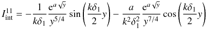
we use integration by parts to approximate the first integral and write
(A.8)Now
we use integration by parts to approximate the first integral and write ![\appendix \setcounter{section}{1} \begin{eqnarray} I_{\rm int}^{11}&=&-\frac{1}{k\delta_1}\frac{{\rm e}^{a\sqrt{y}}}{y^{5/4}}\sin\left(\frac{k\delta_1}{2}y\right)\nonumber \\ &&- \frac{1}{k\delta_1} \int \left[\frac{a}{2y^{7/4}}-\frac{5}{4y^{9/4}}\right]{\rm e}^{a\sqrt{y}}\sin\left(\frac{k\delta_1}{2}y\right){\rm d}y. \label{eq:A4.5} \end{eqnarray}](/articles/aa/full_html/2011/03/aa16075-10/aa16075-10-eq127.png) (A.9)Since
the variable y is very large, the first term in the above square bracket
dominates over the second term. Applying once more integration by parts we have
(A.9)Since
the variable y is very large, the first term in the above square bracket
dominates over the second term. Applying once more integration by parts we have
![\appendix \setcounter{section}{1} \begin{equation} +\frac{a}{k^2\delta_1^2}\int\left[\frac{a}{2y^{9/4}}-\frac{7}{4y^{11/4}}\right] {\rm e}^{a\sqrt{y}}\cos\left(\frac{k\delta_1}{2}y\right) {\rm d}y. \label{eq:A4.6} \end{equation}](/articles/aa/full_html/2011/03/aa16075-10/aa16075-10-eq130.png) (A.10)Using again the
approximation of large y it is obvious that the first term of the above
square bracket is larger than the second term, so we are going to neglect the second term.
The integral on the right-hand side of Eq. (A.10) can be taken to the left-hand side so
(A.10)Using again the
approximation of large y it is obvious that the first term of the above
square bracket is larger than the second term, so we are going to neglect the second term.
The integral on the right-hand side of Eq. (A.10) can be taken to the left-hand side so
![\appendix \setcounter{section}{1} $$ \int a^{a\sqrt{y}}\cos \left(\frac{k\delta_1}{2}y\right)\left[-\frac{1}{2y^{5/4}}-\frac{a^2}{k^2\delta_1^2y^{9/4}}\right]{\rm d}y\approx $$](/articles/aa/full_html/2011/03/aa16075-10/aa16075-10-eq131.png)
 (A.11)Now comparing the terms
on the left-hand side of the above equation it is clear that the second term of the square
bracket can be neglected, so the term remaining on the left-hand side of Eq. (A.11) is exactly the starting form of
(A.11)Now comparing the terms
on the left-hand side of the above equation it is clear that the second term of the square
bracket can be neglected, so the term remaining on the left-hand side of Eq. (A.11) is exactly the starting form of
 , therefore
  (A.12)For the second integral,
 we will need to apply the
same integration by parts which leads to
we will need to apply the
same integration by parts which leads to
 Now turning to the second
integral of Eq. (A.5) a similar procedure
can be employed as above to obtain
Now turning to the second
integral of Eq. (A.5) a similar procedure
can be employed as above to obtain

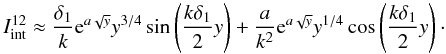
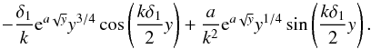 (A.13)Adding together the above
integrals (in the sense of
(A.13)Adding together the above
integrals (in the sense of  we obtain the approximate
value of the integral defined by Eq. (A.3)
which gives the x-dependence of the pressure in the
x < x0 region. A similar
mathematical calculation is needed for the integral defined by Eq. (A.4) describing the
x-dependence of the pressure in the
x > x0 region.
we obtain the approximate
value of the integral defined by Eq. (A.3)
which gives the x-dependence of the pressure in the
x < x0 region. A similar
mathematical calculation is needed for the integral defined by Eq. (A.4) describing the
x-dependence of the pressure in the
x > x0 region.
Returning to the original variable (x), the approximate expressions for the pressure in the two regions become
![\appendix \setcounter{section}{1} $$ p_1(x)\approx {\cal A}\frac{{\rm i}\Lambda\omega\rho_{\odot}{\rm e}^{2/\gamma x}c_{\rm S1}{\rm e}^{a/x}x^{5/2}}{2k\delta_1{\rm e}^{2/x_{\odot}}}\exp\left[-\frac{{\rm i}k\delta_1}{2x^2}\right] $$](/articles/aa/full_html/2011/03/aa16075-10/aa16075-10-eq141.png)
![\appendix \setcounter{section}{1} \begin{equation} \times\left[{\rm i}\left(1-\frac{\delta_1^2}{x^4}\right)+ \frac{ax}{k\delta_1}\left(1-\frac{\delta_1^2}{x^4}\right)\right], \label{eq:A5} \end{equation}](/articles/aa/full_html/2011/03/aa16075-10/aa16075-10-eq142.png)
![\appendix \setcounter{section}{1} $$ p_2(x)\approx {\cal B}\frac{{\rm i}\Lambda\omega\alpha\rho_{i}{\rm e}^{2/\gamma x}c_{\rm S2}{\rm e}^{a/x}x^{5/2}}{2k\delta_2{\rm e}^{2/x_{0}}}\exp\left[\frac{{\rm i}k\delta_2}{2x^2}\right] $$](/articles/aa/full_html/2011/03/aa16075-10/aa16075-10-eq143.png)
![\appendix \setcounter{section}{1} \begin{equation} \times\left[{\rm i} \left(1-\frac{\delta_2^2}{x^4}\right)-\frac{a}{2k\delta_2}\left(1-\frac{\delta_2^2}{x^4}\right)\right]\cdot \label{eq:A6} \end{equation}](/articles/aa/full_html/2011/03/aa16075-10/aa16075-10-eq144.png) (A.15)These expressions will be
used when equating the radial components of the magnetic field perturbation (Eqs. (16) and (17)) in
(A.15)These expressions will be
used when equating the radial components of the magnetic field perturbation (Eqs. (16) and (17)) in
order to derive the dispersion relation of waves propagating near the solar surface.
All Figures
|
Fig. 1 A schematic representation of our working model. Here the gravitational force, Fg, acts in the radial direction towards the center of the Sun, the equilibrium magnetic field, B0, is radial and the density interface at the distance x0 separates two plasma regions labelled by index “1′′ and “2′′ . |
| In the text | |
|
Fig. 2 A selection of density profiles for various values of the density contrast parameter α. For this particular plot the density interface is situated at the distance x0 = 0.19546. |
| In the text | |
|
Fig. 3 The variation of the frequency of global waves propagating as magnetoacoustic-gravity waves at an interface situated at the distance x0 = 0.195 above the solar surface, in terms of the density jump at the interface and the sound speed, cS2, in the second region. |
| In the text | |
|
Fig. 4 The same as in Fig. 2, but now the varying parameters are the density contrast and the location of the density interface, with all the other parameters kept constant. |
| In the text | |
Current usage metrics show cumulative count of Article Views (full-text article views including HTML views, PDF and ePub downloads, according to the available data) and Abstracts Views on Vision4Press platform.
Data correspond to usage on the plateform after 2015. The current usage metrics is available 48-96 hours after online publication and is updated daily on week days.
Initial download of the metrics may take a while.