| Issue |
A&A
Volume 527, March 2011
|
|
|---|---|---|
| Article Number | A87 | |
| Number of page(s) | 26 | |
| Section | Cosmology (including clusters of galaxies) | |
| DOI | https://doi.org/10.1051/0004-6361/201015685 | |
| Published online | 31 January 2011 | |
Combining perturbation theories with halo models
1
Institut de Physique Théorique, CEA Saclay,
91191
Gif-sur-Yvette,
France
e-mail: This email address is being protected from spambots. You need JavaScript enabled to view it.
2
Institute for the Physics and Mathematics of the Universe,
University of Tokyo, Kashiwa,
277-8568
Chiba,
Japan
Received:
3
September
2010
Accepted:
11
December
2010
Abstract
Aims. We investigate the building of unified models that can predict the matter-density power spectrum and the two-point correlation function from very large to small scales, being consistent with perturbation theory at low k and with halo models at high k.
Methods. We use a Lagrangian framework to re-interpret the halo model and to decompose the power spectrum into “2-halo” and “1-halo” contributions, related to “perturbative” and “non-perturbative” terms. We describe a simple implementation of this model and present a detailed comparison with numerical simulations, from k ~ 0.02 up to 100 h Mpc-1, and from x ~ 0.02 up to 150 h-1 Mpc.
Results. We show that the 1-halo contribution contains a counterterm that ensures a k2 tail at low k and this contribution is important not to spoil the predictions on the scales probed by baryon acoustic oscillations, k ~ 0.02 to 0.3 h Mpc-1. On the other hand, we show that standard perturbation theory is inadequate for the 2-halo contribution, because higher order terms grow too fast at high k, so that resummation schemes must be used. Moreover, we explain why such a model, which is based on the combination of perturbation theories and halo models, remains consistent with standard perturbation theory up to the order of the resummation scheme. We describe a simple implementation, based on a 1-loop “direct steepest-descent” resummation for the 2-halo contribution that allows fast numerical computations, and we check that we obtain a good match to simulations at low and high k. We also study the dependence of such predictions on the details of the underlying model, such as the choice of the perturbative resummation scheme or the properties of halo profiles. Our simple implementation already fares better than both standard 1-loop perturbation theory on large scales and simple fits to the power spectrum at high k, with a typical accuracy of 1% on large scales and 10% on small scales. We obtain similar results for the two-point correlation function. However, there remains room for improvement on the transition scale between the 2-halo and 1-halo contributions, which may be the most difficult regime to describe.
Key words: large-scale structure of Universe
© ESO, 2011
1. Introduction
In the standard cosmological scenario, the large-scale structures we observe in the recent Universe (galaxies, clusters, filaments, voids, etc.) have formed through the amplification by gravitational instability of small primordial perturbations generated in the primordial Universe by quantum fluctuations (Peebles 1980). Moreover, at the beginning of matter domination (z ~ 3000), the power increases on small scales for cold dark matter (CDM) models (Peebles 1982), which leads to a “hierarchical scenario” where smaller scales become nonlinear first. Then, increasingly large and massive structures form in the course of time, as small structures merge and larger scales turn nonlinear. Therefore, on large scales or at early times, it is possible to use linear theory or, more generally, perturbation theory, while on small scales or at late times one must use numerical simulations or phenomenological models. One very interesting quantity for characterizing the density fields built by these processes is the density power spectrum P(k), which is the Fourier transform of the density two-point correlation function. On very large linear scales this is actually sufficient for fully determining the statistical properties of the matter distribution if the initial conditions are (almost) Gaussian, as in standard scenarios of single-field inflation. On smaller nonlinear scales, higher order correlations are generated by the nonlinearities of the dynamics, but P(k) remains a standard tool for comparing observations with theoretical predictions (since higher order statistics are increasingly noisy or difficult to predict).
When one focuses on large scales, several observational probes, such as weak lensing surveys (Massey et al. 2007; Munshi et al. 2008), or galaxy redshift surveys provide rich cosmological information. For example, the signature of baryon acoustic oscillations (BAO) (Eisenstein et al. 1998, 2005), redshift-space distortions (Hamilton 1992; Percival & White 2009), non-Gaussianities in the primordial perturbations (Liguori et al. 2010; Desjacques & Seljak 2010), and the mass of neutrinos (Swanson et al. 2010; Saito et al. 2010) are sensitive to the clustering on linear to weakly nonlinear scales, where the departures from the linear regime are already noticeable but still modest. To match the accuracy of future observations a theoretical accuracy on the order of 1% is required, which is beyond the reach of simple phenomenological models or fits to numerical simulations (if one wishes to obtain robust predictions for a wide range of initial conditions and cosmological parameters). However, this regime should be within the range of validity of perturbation theories, which offer the advantage of systematic and reliable predictions, without fitting parameters. This has led to a renewed interest in perturbative approaches in recent years, as it may be possible to improve over the standard perturbation theory (Goroff et al. 1986; Bernardeau et al. 2002) by using resummation schemes that allow partial resummations of higher order terms (Crocce & Scoccimarro 2006b,a; Valageas 2007a; Matarrese & Pietroni 2007; Taruya & Hiramatsu 2008; Valageas 2008; Pietroni 2008; Matsubara 2008). In particular, this somewhat improves the accuracy of the predicted matter power spectrum on the large scales associated with BAO, as compared with standard perturbation theory truncated at the same order (Crocce & Scoccimarro 2008; Carlson et al. 2009; Taruya et al. 2009).
On the other hand, many observational probes, such as weak lensing surveys on smaller angular scales and galaxy surveys, are sensitive to highly nonlinear scales. There, systematic analytical approaches that have been proposed so far do not apply, in particular because of the importance of shell crossing effects that are not adequately taken into account (an exception is the formalism developed in Valageas 2004, which does not make the single-stream approximation since it deals with the phase-space distribution f(x,v;t), but leads to heavy computations). Then, one must resort to numerical simulations or to phenomenological models. One such model is the Lagrangian mapping presented in Hamilton et al. (1991; see Peacock & Dodds 1996, in Fourier space), that writes the nonlinear two-point correlation or power spectrum in terms of its linear counterpart on a different scale. A second model is the “halo model” (Scherrer & Bertschinger 1991; Cooray & Sheth 2002), where the matter distribution is described as a collection of halos. This yields two contributions for the power spectrum or two-point correlation function, a “1-halo” term associated with particle pairs that belong to the same halo, and a “2-halo” term associated with particles that belong to two different halos. Then, the 1-halo term, which dominates on small scales, is sensitive to the density profile and mass distribution of the halos, whereas the 2-halo term, which dominates on large scales, is sensitive to the correlation between halos. In practice, one often replaces the 2-halo term by the linear two-point correlation, or power spectrum, to reproduce linear theory on large scales. Previous works (Cooray & Sheth 2002; Smith et al. 2003, 2007; Giocoli et al. 2010) have shown that halo models provide a good match to numerical simulations, especially at high k, whereas Lagrangian mappings based on the stable clustering ansatz (Peebles 1980) do not fare as well.
It is clear that it is of great interest to develop unified models, which combine the benefits of systematic perturbation theories on large scales with the reasonable match to simulations on small scales provided by halo models. The goal of the present paper is precisely to investigate the building of such a model, that describes all scales, from the linear to the highly nonlinear regime. We can already note here two points that must be addressed to reach this goal: i) the increasingly large growth at high k of higher order terms obtained within standard perturbation theory, and ii) the nonzero limit for k → 0 of the 1-halo term (as written in previous works), which eventually becomes non-negligible (and even dominant) on large scales, since the linear power spectrum typically scales as PL(k) ~ k at low k for CDM scenarios. Thus, the standard implementations of both frameworks are badly behaved beyond their regime of validity, where they should actually become negligible.
In this work we address these issues, and we perform a detailed comparison between different possible implementations of such a unified model, as well as with numerical simulations, as follows. We first consider the computation of the density power spectrum from a Lagrangian point of view in Sect. 2. This provides a decomposition over 2-halo and 1-halo terms that are slightly different from the versions found in previous works, and we emphasize their relationship with “perturbative” and “non-perturbative” terms. In particular, we explain why the 1-halo contribution contains a counterterm, missed in previous studies, that ensures that it becomes truly negligible on large scales, solving the second point ii) above. Next, we present a simple implementation of this model in Sect. 3, and we explain how the point i) above is solved by using resummation schemes instead of the standard perturbation theory. We describe in Sect. 4 the N-body simulations that we use to evaluate the accuracy of our models, and we perform detailed comparisons for the nonlinear density power spectrum in Sect. 5, from k ~ 0.02 h Mpc-1 up to k ~ 100 h Mpc-1, and for redshifts z = 0.35 up to z = 3. Then, we investigate in Sect. 6 the dependence of our results on various ingredients of the model, such as the properties of virialized halos or the choice of the perturbative resummation scheme. We also evaluate the importance of the 1-halo counterterm on large scales. Next, we consider the real-space two-point correlation function in Sect. 7. Finally, we estimate in Sect. 8 the accuracy of such unified models, for both the power spectrum and the two-point correlation, and we conclude in Sect. 9.
In this paper we neglect the impact of baryonic physics on the matter power spectrum, or more precisely we do not explicitly address this issue. Thus, we assume that it can be incorporated in an effective manner through the choice of the halo density profile that enters the model.
2. Decomposition of the density power spectrum from a Lagrangian point of view
We show in this section how the density power spectrum can be split into “perturbative” and “non-perturbative” terms, and how they are related to the 2-halo and 1-halo terms, from a Lagrangian point of view.
2.1. “Perturbative” and “non-perturbative” terms
Let us recall that in a Lagrangian framework one considers the trajectories
x(q,t) of
all particles, of initial Lagrangian coordinates q and
Eulerian coordinates x at time t. In
particular, at any given time t, this defines a mapping,
q → x, from Lagrangian to
Eulerian space, which fully determines the Eulerian density
field ρ(x) through the conservation of
matter,  (1)where
  is the mean
comoving matter density of the Universe and we work in comoving coordinates. Then,
defining the density contrast as
is the mean
comoving matter density of the Universe and we work in comoving coordinates. Then,
defining the density contrast as  (2)and its Fourier
transform as
(2)and its Fourier
transform as 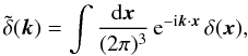 (3)we obtain from Eq. (1)
 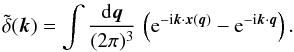 (4)Next, defining the
density power spectrum as
(4)Next, defining the
density power spectrum as 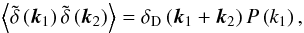 (5)we obtain from
Eq. (4), using statistical homogeneity,
(5)we obtain from
Eq. (4), using statistical homogeneity,
 (6)where we introduced
the Eulerian-space separation Δx,
(6)where we introduced
the Eulerian-space separation Δx,  (7)The expression (6) is fully general since it is a simple
consequence of the matter conservation Eq. (1), and of statistical homogeneity. In particular, it holds for any dynamics,
such as the one associated with the Zeldovich approximation (Zeldovich 1970). There, the
mapping x(q) is given by
the linear displacement field ΨL, as
x(q) = q + ΨL(q),
so that for Gaussian initial conditions (i.e.
ΨL(q) is Gaussian)
one can easily compute the average (6) and
derive an explicit analytic expression for the density power spectrum (Schneider & Bartelmann 1995; Taylor & Hamilton 1996; Valageas 2010a).
(7)The expression (6) is fully general since it is a simple
consequence of the matter conservation Eq. (1), and of statistical homogeneity. In particular, it holds for any dynamics,
such as the one associated with the Zeldovich approximation (Zeldovich 1970). There, the
mapping x(q) is given by
the linear displacement field ΨL, as
x(q) = q + ΨL(q),
so that for Gaussian initial conditions (i.e.
ΨL(q) is Gaussian)
one can easily compute the average (6) and
derive an explicit analytic expression for the density power spectrum (Schneider & Bartelmann 1995; Taylor & Hamilton 1996; Valageas 2010a).
The second term in Eq. (6), eik·q, merely gives a Dirac factor, δD(k), and can often be discarded in exact or systematic computations (e.g., perturbative expansions) if one consider k ≠ 0. Within perturbative expansions of P(k) over powers of the linear power spectrum, PL(k), it simply cancels out the zeroth-order term so that P(k) = PL(k) at lowest order. However, as we shall see below, it will prove important in the following analysis to keep track of this factor. Indeed, it will be split over two parts, along with the first term eik·Δx, and it is clear that one should either discard it or keep it in a consistent manner in both parts, contrary to what is implicitly done in usual versions of the halo model.
For the three-dimensional gravitational dynamics it is not possible to derive an explicit analytical expression for the average (6). Therefore, as in the Eulerian framework, one must resort to perturbative expansions (Bouchet et al. 1995; Matsubara 2008) or phenomenological models. In this paper, our goal is precisely to use Eq. (6) as a starting point to decompose the density power spectrum, P(k), over two parts, associated with “perturbative” and “non-perturbative” contributions.
Here and in the following, we call “perturbative” those contributions that can be obtained from perturbative expansions over powers of the linear power spectrum PL(k) within the fluid approximation. In practice, these may be derived from the equations of motion, written in terms of the density and velocity fields in the usual hydrodynamical description of the system, by writing these nonlinear Eulerian fields as perturbative series over powers of the linear growing mode (Goroff et al. 1986; Bernardeau et al. 2002). Partial resummations of this standard perturbative series have been recently introduced (Crocce & Scoccimarro 2006b,a; Valageas 2007a; Matarrese & Pietroni 2007; Taruya & Hiramatsu 2008; Valageas 2008; Pietroni 2008) but remain within this hydrodynamical regime. Of course, it is possible to develop perturbative expansions, and associated resummations, in Lagrangian space (Bouchet et al. 1995; Matsubara 2008), by looking for an expansion of the displacement field Ψ(q) over powers of the linear displacement field. Taken at face value, these schemes imply some shell crossing. For instance, at lowest order one recovers the Zeldovich dynamics for the displacement field. However, this does not mean that they take into account in a systematic fashion the physics beyond shell crossing, which remains beyond the reach of current approaches of this kind. Technically, the gravitational potential is obtained from the Poisson equation, where the density contrast is obtained from the conservation of matter (1) as δ(x) = |det(∂x/∂q)| -1 − 1, and one expands the Jacobian over powers of the displacement Ψ. In doing so, one discards the absolute value and misses the changes of sign that occur after shell crossing. On the other hand, these schemes give the same final expansion over powers of PL for the nonlinear power spectrum as the Eulerian schemes, up to the order of truncation of the computation. Therefore, we consider both perturbative approaches as “perturbative” schemes, in the sense of expansions over powers of PL that neglect shell crossing. By contrast, we call “non-perturbative” those contributions that cannot be obtained through these approaches, either because they are beyond the reach of perturbative expansions (such as factors of the form e−1/PL that cannot be uncovered by Taylor series over PL) or because they arise from the behavior of the system beyond shell crossing (and require going beyond the single-stream approximation).
In Valageas (2010a) such a decomposition between
perturbative and non-perturbative contributions to the density power spectrum was obtained
within the framework of the Zeldovich dynamics. More precisely, a “sticky model” that only
differs from the Zeldovich dynamics beyond shell crossing was introduced. Then, whereas
the Zeldovich density power spectrum is exactly given by a resummation of perturbative
terms (i.e., the non-perturbative contribution is zero), the “sticky model” power spectrum
contains an additional non-perturbative contribution, while its perturbative part is
identical to the one of the Zeldovich dynamics. Inspired by this simpler example, we
perform a similar decomposition of Eq. (6)
over perturbative and non-perturbative contributions. However, we no longer have a simple
criterion to distinguish particle pairs that have undergone shell crossing, because for
the gravitational dynamics even at the perturbative level (at third order) the
displacement field develops rotational terms (Buchert
1994; Bernardeau & Valageas 2008).
Therefore, we use a phenomenological halo model, in the sense that we assume that the
matter distribution can be described as a collection of spherical halos defined by a given
nonlinear density contrast δ. As usual, we can write the halo mass
function as  (8)in terms of a
scaling function f(ν) and of the reduced
variable ν. Here, σ(M) is the rms
linear density contrast at scale M, or Lagrangian
radius qM, with
(8)in terms of a
scaling function f(ν) and of the reduced
variable ν. Here, σ(M) is the rms
linear density contrast at scale M, or Lagrangian
radius qM, with  (9)and
  (10)where
 is the Fourier transform of
the top-hat of radius q, defined as
is the Fourier transform of
the top-hat of radius q, defined as 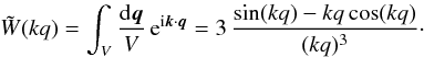 (11)In the second Eq. (8) the linear density
contrast δL is related to the nonlinear density
threshold δ that defines the halos through the spherical collapse
dynamics (Valageas 2009a),
(11)In the second Eq. (8) the linear density
contrast δL is related to the nonlinear density
threshold δ that defines the halos through the spherical collapse
dynamics (Valageas 2009a),  (12)and for Gaussian
initial conditions the large-mass tail shows the exponential falloff
(12)and for Gaussian
initial conditions the large-mass tail shows the exponential falloff ![Mathematical equation: \begin{equation} \nu \rightarrow \infty : \;\; \ln[f(\nu)] \sim -\frac{\nu^2}{2}, \label{nu-tail} \end{equation}](/articles/aa/full_html/2011/03/aa15685-10/aa15685-10-eq64.png) (13)whence
(13)whence 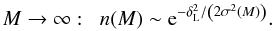 (14)This corresponds to the
Press-Schechter falloff (Press & Schechter
1974), but with a somewhat lower threshold δL given
by Eq. (12) (the usual Press-Schechter
threshold actually corresponds to δL = ℱ-1(∞),
associated with full collapse to a point). However, the relation (12) only holds for
δ < δvir, which typically gives
δ < 200, as larger density contrasts are associated with inner
shells where shell crossing plays a key role and modifies Eq. (12), associated with spherical dynamics at
constant mass (Valageas 2009a). On the other hand,
the halo mass function satisfies the normalization
(14)This corresponds to the
Press-Schechter falloff (Press & Schechter
1974), but with a somewhat lower threshold δL given
by Eq. (12) (the usual Press-Schechter
threshold actually corresponds to δL = ℱ-1(∞),
associated with full collapse to a point). However, the relation (12) only holds for
δ < δvir, which typically gives
δ < 200, as larger density contrasts are associated with inner
shells where shell crossing plays a key role and modifies Eq. (12), associated with spherical dynamics at
constant mass (Valageas 2009a). On the other hand,
the halo mass function satisfies the normalization 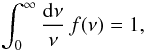 (15)which ensures
that all the mass is contained within such halos (for linear power spectra such
that σ(q) grows to infinity on small scales). This
also ensures that there is no overcounting (as would be the case if one used a mass
function with a normalization greater than unity).
(15)which ensures
that all the mass is contained within such halos (for linear power spectra such
that σ(q) grows to infinity on small scales). This
also ensures that there is no overcounting (as would be the case if one used a mass
function with a normalization greater than unity).
Then, in Lagrangian space, the probability dF for one
particle q1 to belong to a halo of mass in
the range [M,M + dM] reads as 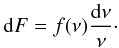 (16)This is also the fraction
of matter enclosed within such halos. Next, making the approximation that each halo comes
from an initial spherical region in Lagrangian space, the probability for a second
particle q2, at distance
q = |q2 − q1| ,
to belong to the same halo reads as
(16)This is also the fraction
of matter enclosed within such halos. Next, making the approximation that each halo comes
from an initial spherical region in Lagrangian space, the probability for a second
particle q2, at distance
q = |q2 − q1| ,
to belong to the same halo reads as  (17)Here we integrate
over all positions q1 within the spherical
volume V of radius qM, and
we integrate over all directions Ωq
of the Lagrangian vector
q = q2 − q1.
The top-hat factor
θ(q2 ∈ V) is
unity if q2 is located within the
volume V, and zero otherwise. By isotropy the result only depends on
the length q, and performing the integrations yields
(17)Here we integrate
over all positions q1 within the spherical
volume V of radius qM, and
we integrate over all directions Ωq
of the Lagrangian vector
q = q2 − q1.
The top-hat factor
θ(q2 ∈ V) is
unity if q2 is located within the
volume V, and zero otherwise. By isotropy the result only depends on
the length q, and performing the integrations yields  (18)and
FM(q) = 0 for
q > 2qM. Therefore,
combining Eqs. (16) and (18), we obtain the probability that a pair of
particles of Lagrangian separation q belongs to the same halo of
mass M as
(18)and
FM(q) = 0 for
q > 2qM. Therefore,
combining Eqs. (16) and (18), we obtain the probability that a pair of
particles of Lagrangian separation q belongs to the same halo of
mass M as  (19)and
dFq(M) = 0 for
qM < q/2. In
particular, the probability that the pair
{ q1,q2 }
belongs to a single halo writes as
(19)and
dFq(M) = 0 for
qM < q/2. In
particular, the probability that the pair
{ q1,q2 }
belongs to a single halo writes as  (20)where νq/2
is defined as in Eq. (8), for the
Lagrangian radius
qM = q/2. On the other
hand, the probability F2H(q) that the
Lagrangian pair does not belong to a single halo (whence the two points belong to two
different halos) reads as
(20)where νq/2
is defined as in Eq. (8), for the
Lagrangian radius
qM = q/2. On the other
hand, the probability F2H(q) that the
Lagrangian pair does not belong to a single halo (whence the two points belong to two
different halos) reads as  (21)Then, we split the
average in Eq. (6) over two terms,
P1H and P2H, associated with
pairs { 0,q } that belong to a single halo or to two
different halos,
(21)Then, we split the
average in Eq. (6) over two terms,
P1H and P2H, associated with
pairs { 0,q } that belong to a single halo or to two
different halos,  (22)with
  (23)and
 (24)Here the averages
⟨ ... ⟩ 1H and ⟨ ... ⟩ 2H are
the conditional averages, knowing that the pair of length q belongs to a
single halo or to two halos. The decomposition (22) clearly corresponds to the 1-halo and 2-halo terms of the usual halo model
(Cooray & Sheth 2002). Then, to make the
connection with the distinction between perturbative and non-perturbative terms, we note
that at a perturbative level F1H is identically zero
and F2H unity,
(24)Here the averages
⟨ ... ⟩ 1H and ⟨ ... ⟩ 2H are
the conditional averages, knowing that the pair of length q belongs to a
single halo or to two halos. The decomposition (22) clearly corresponds to the 1-halo and 2-halo terms of the usual halo model
(Cooray & Sheth 2002). Then, to make the
connection with the distinction between perturbative and non-perturbative terms, we note
that at a perturbative level F1H is identically zero
and F2H unity,  (25)Indeed,
the large-mass tail (14) is actually a
rare-event limit that holds both in the large-mass limit, at fixed linear density power
spectrum (Valageas 2002b, 2009a), and in the quasi-linear limit at fixed mass, where the
amplitude of the linear density power spectrum goes to zero (Valageas 2002a, 2009a). It is
this second regime which corresponds to usual perturbation theories, where as recalled
above we look for expansions over powers of the amplitude of the linear power spectrum.
Then, because of the exponential decay of the form
e − 1/σ2(M) we can see that
the expansion over powers of PL
of F1H(q) defined in Eq. (20), at fixed q, is
identically zero. From Eq. (21) this also
yields F2H = 1 at all orders of perturbation theory.
Therefore, we can see from Eqs. (23),
(24) that the 1-halo contribution is a
fully non-perturbative term, while the 2-halo contribution is (almost) the perturbative
term multiplied by the factor F2H(q).
(25)Indeed,
the large-mass tail (14) is actually a
rare-event limit that holds both in the large-mass limit, at fixed linear density power
spectrum (Valageas 2002b, 2009a), and in the quasi-linear limit at fixed mass, where the
amplitude of the linear density power spectrum goes to zero (Valageas 2002a, 2009a). It is
this second regime which corresponds to usual perturbation theories, where as recalled
above we look for expansions over powers of the amplitude of the linear power spectrum.
Then, because of the exponential decay of the form
e − 1/σ2(M) we can see that
the expansion over powers of PL
of F1H(q) defined in Eq. (20), at fixed q, is
identically zero. From Eq. (21) this also
yields F2H = 1 at all orders of perturbation theory.
Therefore, we can see from Eqs. (23),
(24) that the 1-halo contribution is a
fully non-perturbative term, while the 2-halo contribution is (almost) the perturbative
term multiplied by the factor F2H(q).
The factor F1H being non-perturbative is not mainly related to shell crossing, but simply to the fact that it cannot be recovered by a series expansion over powers of PL. However, for halos that would be defined by a high density threshold, typically δ > 200, the exponential falloff (14) is modified by shell crossing (i.e. the factor δL is no longer given by Eq. (12), see Valageas 2009a) so that it would also be non-perturbative in this sense. On the other hand, even for lower threshold δ, the exact form of the factor F1H(q), and in particular the low-mass tail of the halo mass function, depends on the behavior of the system beyond shell crossing.
The decomposition (22), with the Lagrangian-based interpretation (23) − (24), has the advantage to automatically satisfy the conservation of matter. Thus, thanks to Eq. (21) we count all particle pairs once. By contrast, in the Eulerian derivation of the halo model, where we first write the density field ρ(x) as a sum of halo profiles, we would need to pay attention to possible overlaps between halos, which arise when we use a spherical approximation. Thus, the splitting (22) is more easily expressed in this framework, and one can independently focus on the modelization of the averages ⟨ eik·Δx − eik·q ⟩ . The latter also offers a closer link to the dynamics, through the mapping q → x. We shall not make much use of this relationship in the following, as we use simple approximations that allow us to recover the usual Eulerian expressions, with the addition of simple prefactors and counterterms, but this may provide a route to more accurate modeling.
2.2. “2-halo” contribution
We first consider the 2-halo contribution (24). Since the conditional average involves the constraint that the pair
{ 0,q } does not belong to the same halo, the mean of
eik·Δx is
“biased” as compared with a mean over all possible pairs. However, in order to simplify
the computation of this term, we note that at a perturbative level
F2H = 1, as seen in (25), so that we can replace the average
⟨ ... ⟩ 2H by the mean over all pairs, as given by
perturbation theory,  (26)where the subscript
“pert” denotes quantities obtained from standard perturbation theory (or equivalently its
various resummation schemes). Thus Eq. (26) is still exact at all orders of perturbation theory. This expression is best
suited for perturbation theories developed within the Lagrangian framework. Unfortunately,
as we shall discuss in Sect. 6.5 below, Lagrangian
perturbation theories built so far are not as efficient as their Eulerian counterparts,
especially when we consider available resummation schemes. Then, in order to make contact
with Eulerian perturbation theories we further approximate Eq. (26) as
(26)where the subscript
“pert” denotes quantities obtained from standard perturbation theory (or equivalently its
various resummation schemes). Thus Eq. (26) is still exact at all orders of perturbation theory. This expression is best
suited for perturbation theories developed within the Lagrangian framework. Unfortunately,
as we shall discuss in Sect. 6.5 below, Lagrangian
perturbation theories built so far are not as efficient as their Eulerian counterparts,
especially when we consider available resummation schemes. Then, in order to make contact
with Eulerian perturbation theories we further approximate Eq. (26) as  (27)where
we have replaced the q-dependent
factor F2H(q) by its value at a typical
scale q ~ 1/k. Again, this is legitimate at a
perturbative level, where F2H = 1, so that Eq. (27) remains exact at all orders of
perturbation theory. To obtain the second line we simply used the exact expression (6), which implies the same equality in terms of
perturbative expansions.
(27)where
we have replaced the q-dependent
factor F2H(q) by its value at a typical
scale q ~ 1/k. Again, this is legitimate at a
perturbative level, where F2H = 1, so that Eq. (27) remains exact at all orders of
perturbation theory. To obtain the second line we simply used the exact expression (6), which implies the same equality in terms of
perturbative expansions.
Let us recall that from (25) the 1-halo contribution is zero at all orders of perturbation theory, so that the full power spectrum P(k) of Eq. (22) automatically agrees with perturbation theory at all orders, whether we use Eq. (26) or (27). Then, within these approximations the only effect of non-perturbative corrections to the 2-halo term is to multiply the perturbative power spectrum Ppert(k) by the prefactor F2H(1/k).
Within the usual halo model the 2-halo term reads as (Cooray & Sheth 2002)  (28)where
  is the normalized halo
density profile, defined in Eq. (31)
below, and
PM1M2(k)
is the halo power spectrum. The second line (28) is obtained in the low-k limit, so that
is the normalized halo
density profile, defined in Eq. (31)
below, and
PM1M2(k)
is the halo power spectrum. The second line (28) is obtained in the low-k limit, so that
 and
PM1M2(k) ≃ b(M1)b(M2)PL(k),
with a halo bias b(M) that is normalized to unity. It is
also possible to combine perturbation theory and nonlinear halo bias to make the
expression above consistent with standard perturbation theory while building a model for
the halo power spectrum itself, see Smith et al.
(2007).
and
PM1M2(k) ≃ b(M1)b(M2)PL(k),
with a halo bias b(M) that is normalized to unity. It is
also possible to combine perturbation theory and nonlinear halo bias to make the
expression above consistent with standard perturbation theory while building a model for
the halo power spectrum itself, see Smith et al.
(2007).
Of course, in order to describe the weakly nonlinear regime one can as well replace PL(k) by Ppert(k) in Eq. (28), which gives an expression very similar to Eq. (27). Then, we can see that a first difference between the halo-model expression (28) and Eq. (27) is that we did not need to introduce any halo bias to derive Eq. (27). In fact, although the contribution (24) is associated with a 2-halo term, by making the simple approximation (26) we avoid any need to consider halo biasing, and as explained above this does not spoil the agreement with perturbation theory. The second difference is the prefactor F2H(1/k) in Eq. (27). As seen from Eq. (6) and the splitting (22), this term is required by self-consistency, to ensure that the two averages F1H(q) ⟨ eik·Δx ⟩ 1H and F2H(q) ⟨ eik·Δx ⟩ 2H sum up to ⟨ eik·Δx ⟩ , and in particular that they sum up to unity for k → 0. Within the usual halo model, this factor is implicitly set to unity by taking the large-scale limit in Eq. (28) and ignoring exclusion constraints on the halos. This is also valid within perturbation theory, as seen in (25). However, in order to describe the weakly nonlinear regime, where the 1-halo term is nonzero, it is best to keep the prefactor F2H(1/k) in Eq. (27), to keep a consistent model and to avoid any overcounting.
2.3. “1-halo” contribution
From Eqs. (20) and (23) the 1-halo contribution to the density
power spectrum reads as  (29)In
order to compute the average in Eq. (29),
within a halo of mass M, we make the approximation of fully virialized
spherical halos. Thus, we describe the halos as spherical objects, truncated at a
radius rM such that the mean density
contrast within this radius is the nonlinear threshold δ used to define
these objects, and the enclosed mass is equal to M,
(29)In
order to compute the average in Eq. (29),
within a halo of mass M, we make the approximation of fully virialized
spherical halos. Thus, we describe the halos as spherical objects, truncated at a
radius rM such that the mean density
contrast within this radius is the nonlinear threshold δ used to define
these objects, and the enclosed mass is equal to M,  (30)We introduce as usual
the normalized Fourier transform of this halo radial profile,
(30)We introduce as usual
the normalized Fourier transform of this halo radial profile,  (31)where
ρM(x) is the halo
density profile. Next, using the approximation of fully virialized halos, that is, that
the two Lagrangian particles “0” and “q” have lost all
memory of their initial locations and are independently located at random within the halo,
we write
(31)where
ρM(x) is the halo
density profile. Next, using the approximation of fully virialized halos, that is, that
the two Lagrangian particles “0” and “q” have lost all
memory of their initial locations and are independently located at random within the halo,
we write  Substituting
into Eq. (29) and exchanging the order of
integration gives
Substituting
into Eq. (29) and exchanging the order of
integration gives  (34)and
the integration over q yields
(34)and
the integration over q yields  (35)Therefore, we recover
the usual 1-halo term of the halo model (Cooray &
Sheth 2002), with the addition of the new counterterm
(35)Therefore, we recover
the usual 1-halo term of the halo model (Cooray &
Sheth 2002), with the addition of the new counterterm
 ,
where
,
where  was defined in Eq. (11).
This counterterm originates from the second term in Eq. (6), which actually sums up to a Dirac factor δD(k). However, since we eventually split the nonlinear power spectrum as in Eq. (22) and we use different approximations for the 2-halo and 1-halo contributions, it is best to keep track of this factor in both contributions. In particular, as pointed out in Sect. 2.1, one should avoid keeping it in one contribution and disregarding it in the other one. Thus, it has been explicitly used in Eq. (27) to cancel out the zeroth-order term F2HδD(k), so that one should keep it in the 1-halo term (23). Within the usual halo model this term is usually missed because the splitting between the 2-halo and 1-halo terms is not treated so carefully. In particular, as noticed in Sect. 2.2, the usual halo model implicitly takes F2H = 1 (which is valid in perturbation theory) while taking F1H ≠ 0 by adding the 1-halo term, which is not fully consistent.
In fact, the counterterm of Eq. (35) can
be recovered without going through the previous steps, associated with a Lagrangian point
of view, by the following simple argument. Let us consider a uniform universe, where there
are no density fluctuations and the density is everywhere equal
to . Then,
within the spirit of the usual (Eulerian) halo model, and making the same approximations
(e.g., neglecting geometrical constraints, associated with exclusion constraints, and
departures from spherical symmetry), we can consider that all the matter is within halos
of constant density with an
arbitrary distribution of halo radii. That is, we can split this uniform system over an
arbitrary set of cells, which we can call halos. Then, within such a halo model the usual
1-halo term for the full density correlation,  (defined as
 , as in Eq. (5)), reads as the counterterm of Eq. (35), with a positive sign and multiplied
by
, as in Eq. (5)), reads as the counterterm of Eq. (35), with a positive sign and multiplied
by  . Indeed, the
density profile of such halos is simply the top-hat of
radius qM, since δ = 0
whence
rM = qM,
so that the normalized Fourier transform of the halo radial profile defined in Eq. (31) is equal to the Fourier transform (11),
. Indeed, the
density profile of such halos is simply the top-hat of
radius qM, since δ = 0
whence
rM = qM,
so that the normalized Fourier transform of the halo radial profile defined in Eq. (31) is equal to the Fourier transform (11),  . This means that within a
halo model, for any halo mass function, the 1-halo contribution to the power spectrum
associated with an uniform-density medium reads as the counterterm of Eq. (35). Since the density-contrast power spectrum
can also be defined as
. This means that within a
halo model, for any halo mass function, the 1-halo contribution to the power spectrum
associated with an uniform-density medium reads as the counterterm of Eq. (35). Since the density-contrast power spectrum
can also be defined as  (i.e. we consider the
connected two-point correlation), we must subtract this uniform-density term as in
Eq. (35), as the first
term
(i.e. we consider the
connected two-point correlation), we must subtract this uniform-density term as in
Eq. (35), as the first
term  corresponds to
the total density power spectrum,
Pρρ(k).
corresponds to
the total density power spectrum,
Pρρ(k).
In agreement with this result, we can note by an integration over k of the second term of Eq. (34) that the second term of Eq. (35) is indeed a well-normalized approximation to δD(k), where the Dirac peak is broadened over a size ~1/qM associated with the typical halo scale (thus, as could be expected, this becomes an increasingly good approximation to δD(k) as the halo size goes to infinity and the associated power is repelled to k → 0). Clearly, the fact that this does not yield exactly a Dirac factor, whence that it does not vanish for nonzero k, is due to the fact that it is only a partial contribution to the full power spectrum, since by construction within such halo models there is always a 2-halo term, and it is only the sum of both contributions that contains such a Dirac factor. (This also agrees with the fact that we recover a Dirac factor in the limit qM → ∞, since at fixed scale 1/k the 2-halo term clearly disappears in this limit.)
In practice, the counterterm of Eq. (35)
is small on most scales of interest, especially in the nonlinear regime. However, it plays
an important role on very large scales. Indeed, since
 we can see that the first
term of Eq. (35), associated with the
usual halo model, goes to a nonzero constant as k → 0. Since for CDM-like
initial power spectra
PL(k) ∝ kns
with ns ≃ 1 as k → 0, this
implies that the usual 1-halo term dominates on very large scale, which is not correct. In
fact, from the conservation of matter a small-scale redistribution of matter generically
yields a P(k) ∝ k2 tail at
low k, while taking into account momentum conservation one obtains
a k4 tail (Peebles
1974). To solve this problem the use of compensated halo profiles (i.e. with
we can see that the first
term of Eq. (35), associated with the
usual halo model, goes to a nonzero constant as k → 0. Since for CDM-like
initial power spectra
PL(k) ∝ kns
with ns ≃ 1 as k → 0, this
implies that the usual 1-halo term dominates on very large scale, which is not correct. In
fact, from the conservation of matter a small-scale redistribution of matter generically
yields a P(k) ∝ k2 tail at
low k, while taking into account momentum conservation one obtains
a k4 tail (Peebles
1974). To solve this problem the use of compensated halo profiles (i.e. with
 ) was investigated in Cooray & Sheth (2002). However, they noticed
that this recipe fails because it also spoils the 2-halo term, as seen from the first line
in Eq. (28). Here we can see that this
problem is automatically solved within our approach by the counterterm
) was investigated in Cooray & Sheth (2002). However, they noticed
that this recipe fails because it also spoils the 2-halo term, as seen from the first line
in Eq. (28). Here we can see that this
problem is automatically solved within our approach by the counterterm
 in Eq. (35). In particular we recover at
low k the expected slope
P1H(k) ∝ k2,
associated with small-scale rearrangements (indeed, the 1-halo term only describes the
redistribution within small clumps, and is not sensitive to the long-range correlations
between clumps, that is described by the 2-halo term).
in Eq. (35). In particular we recover at
low k the expected slope
P1H(k) ∝ k2,
associated with small-scale rearrangements (indeed, the 1-halo term only describes the
redistribution within small clumps, and is not sensitive to the long-range correlations
between clumps, that is described by the 2-halo term).
Looking at the steps of the derivation of Eq. (35) we can also see why we fail to recover the k4
tail due to momentum conservation. Indeed, in the approximation (33), where we have assumed full virialization,
we have erased all memory of the initial positions and velocities of the two Lagrangian
particles { 0,q } , which clearly implies that we have
disregarded the constraints associated with momentum conservation. Therefore, in order to
obtain a k4 tail one should improve this approximation, by
taking care at some level of the particle velocities. Of course, a simpler remedy would be
to modify the counterterm in Eq. (35), by using a window
 that cancels both the
terms k0 and k2
of . However, since
the CDM linear power spectrum roughly behaves as
PL(k) ∝ k at
low k the k2 tail is sufficient to make the
1-halo term subdominant on large scales, as we shall check in Sect. 5 below. Therefore, we shall keep the simple approximation (33) in the following, and Eq. (35) for the 1-halo term, as it appears to be
sufficient to reach a good agreement with numerical simulations.
that cancels both the
terms k0 and k2
of . However, since
the CDM linear power spectrum roughly behaves as
PL(k) ∝ k at
low k the k2 tail is sufficient to make the
1-halo term subdominant on large scales, as we shall check in Sect. 5 below. Therefore, we shall keep the simple approximation (33) in the following, and Eq. (35) for the 1-halo term, as it appears to be
sufficient to reach a good agreement with numerical simulations.
2.4. Extension to the galaxy power spectrum
Although in this article we focus on the dark matter power spectrum, we briefly discuss
in this section how the previous results can be used for the galaxy power spectrum, which
is also a quantity of great practical interest. This necessarily involves additional
ingredients, as we must define the relationship between the dark matter density field and
the galaxies. As usual (Seljak 2000; Cooray & Sheth 2002), we keep the
splitting (22) over 1-halo and 2-halo
terms. Then, we simply write the galaxy 2-halo contribution as 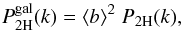 (36)where
⟨ b ⟩ is the mean bias of the galaxy population that we consider.
This can be computed using one of the bias models that have been proposed in previous
works (Mo & White 1996; Sheth & Tormen 1999; Sheth et al. 2001; Valageas
2009a, 2010b) or fits to numerical
simulations (Tinker et al. 2010). Next, following
the Eulerian interpretation of the counterterm of Eq. (35) discussed in the previous section, as arising from the difference
⟨ ngalngal ⟩ − ⟨ ngal ⟩ ⟨ ngal ⟩ ,
we write the 1-halo term as
(36)where
⟨ b ⟩ is the mean bias of the galaxy population that we consider.
This can be computed using one of the bias models that have been proposed in previous
works (Mo & White 1996; Sheth & Tormen 1999; Sheth et al. 2001; Valageas
2009a, 2010b) or fits to numerical
simulations (Tinker et al. 2010). Next, following
the Eulerian interpretation of the counterterm of Eq. (35) discussed in the previous section, as arising from the difference
⟨ ngalngal ⟩ − ⟨ ngal ⟩ ⟨ ngal ⟩ ,
we write the 1-halo term as 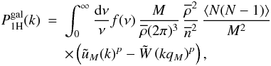 (37)where
 is the mean
galaxy number density, ⟨ N(N − 1) ⟩ is the mean
squared number of galaxies (minus a factor N) in halos of
mass M, and p = 1 or 2 depending on whether the former
quantity is smaller or greater than unity (Seljak
2000; Cooray & Sheth 2002). Thus,
we have simply subtracted to the usual expression the counterterm associated with galaxies
set at random within the Lagrangian radius qM
(i.e., corresponding to a uniform density universe). Again, the quantity
⟨ N(N − 1) ⟩ must be computed from a model defined
for the population of galaxies that we consider.
is the mean
galaxy number density, ⟨ N(N − 1) ⟩ is the mean
squared number of galaxies (minus a factor N) in halos of
mass M, and p = 1 or 2 depending on whether the former
quantity is smaller or greater than unity (Seljak
2000; Cooray & Sheth 2002). Thus,
we have simply subtracted to the usual expression the counterterm associated with galaxies
set at random within the Lagrangian radius qM
(i.e., corresponding to a uniform density universe). Again, the quantity
⟨ N(N − 1) ⟩ must be computed from a model defined
for the population of galaxies that we consider.
The derivation of Eq. (37) is more phenomenological than the derivation of Eq. (35) from the Lagrangian point of view (29). However, since one always needs to introduce some phenomenological model to relate galaxies to the matter distribution (here through the two quantities ⟨ b ⟩ (M) and ⟨ N(N − 1) ⟩ (M)), this should be sufficient.
The contribution (37) to the galaxy power spectrum vanishes as k2 in the large-scale limit, which again solves the unphysical nonzero limit obtained in previous implementations. This behavior remains valid even though galaxies are discrete objects, since this property only implies a constant shot-noise asymptote for Pgal(k) in the high-k limit. This shot-noise has actually been subtracted in Eq. (37), using the quantity ⟨ N(N − 1) ⟩ instead of ⟨ N2 ⟩ , to follow the usual convention (Peebles 1980; Seljak 2000; Cooray & Sheth 2002). At low k, we are dominated by the 2-halo contribution and in case of constant large-scale bias we recover the slope Pgal(k) ∝ kns of the primordial matter power spectrum1.
3. A simple implementation
We describe in more detail in this section how we implement Eqs. (27) and (35) to compute the nonlinear density power spectrum.
3.1. “2-halo” contribution
We first consider the 2-halo contribution (27), and more precisely the perturbative part Ppert(k), as we shall discuss the non-perturbative prefactor F2H(1/k) in Sect. 3.2 below.
Since we cannot compute and resum all terms of the perturbative expansion of P(k), contrary to the simpler Zeldovich dynamics, we must use for Ppert(k) an approximation associated with a truncation at a finite order. This leads to several possible choices, since a priori we can use the standard perturbation theory (Goroff et al. 1986; Bernardeau et al. 2002) as well as any of the various resummation schemes that have been introduced in the recent years (Crocce & Scoccimarro 2006b,a; Valageas 2007a; Matarrese & Pietroni 2007; Valageas 2008; Taruya & Hiramatsu 2008; Pietroni 2008). Indeed, all such methods give expressions for Ppert(k) that agree up to the order of the computation, and only differ by higher order terms.
However, it turns out that standard perturbation theory cannot suit our purposes because higher order terms grow increasingly fast at high k (Bernardeau et al. 2002). As we shall check in Sect. 6.4 below, at one-loop order it already gives a steep contribution that remains non-negligible at high k, because the prefactor F2H(1/k) does not go to zero very fast (because for CDM power spectra σ(q) only grows logarithmically at small q if ns = 1, and even remains finite if ns < 1). This implies that to get a well-behaved 2-halo term we need to use other schemes, that provide a perturbative part Ppert(k) that remains small at high k as compared with the 1-halo term. Therefore, we must use one of the resummation schemes that have been recently developed and show a well-behaved high-k behavior.
It is interesting to point out that, although such approaches were devised in order to improve the accuracy of perturbation theory on large scale and to increase its range of validity (by improving its convergence through partial resummations of an infinite number of higher order terms), our study shows that a second important benefit of these schemes is to provide well-behaved expressions for Ppert(k). Here the point is not that the high-k behavior is accurately reproduced (since anyway perturbation theory does not apply in this range) but that it remains within reasonable bounds (typically close to or smaller than the linear power) so as to be subdominant. Thus, by giving systematic expansions of Ppert(k), which agree with perturbation theory up to the order of the computation while remaining well-behaved at high k, these schemes allow the construction of unified models such as those studied in this article, based on Eq. (22), that show a correct behavior at both low and high k. (In the same spirit, we have checked in Sect. 2.3 that the 1-halo term is well-behaved at low k.) This provides a second important motivation for such resummation schemes, as compared with standard perturbation theory.
In this article we focus on the “direct steepest-descent method” introduced in Valageas (2007a). In terms of diagrams it means that the two-point correlation C is given at one-loop order by the resummations shown in Fig. 1, where single lines are the linear correlation and response functions CL and RL, while the double lines are the nonlinear correlation and response functions C and R obtained at that order, see also Valageas (2008). At this one-loop order the standard perturbation theory consists in keeping only the three diagrams with zero or one bubble among the infinite series shown in the second equality in Fig. 1. We recall the details of the computation of the (perturbative) density power spectrum Ppert(k) within this approach in Appendix A.
 |
Fig. 1 The resummation performed by the “direct steepest-descent” method at one-loop order, for the two-point correlation C. The blue single lines are the linear correlation CL and the red single lines are the linear response (propagator) RL. The double red lines in the first equality are the nonlinear response R (at that order), which contains an infinite series of bubble diagrams, and explicit substitution gives the series of diagrams shown in the second equality below. |
This direct steepest-descent method is not necessarily the most accurate resummation scheme. In particular, it yields a response function that does not decay at high k or late times, but shows increasingly fast oscillations with an amplitude that follows the linear response function. This is not realistic, since one expects a Gaussian-like decay for Eulerian response functions, as can be seen from theoretical arguments and numerical simulations (Crocce & Scoccimarro 2006b,a; Valageas 2007b; Bernardeau & Valageas 2010a). However, the fast oscillations still provide an effective damping in a weak sense (that is when the response function is integrated over). The reason why we consider this direct steepest-descent method here is that it provides a simple and efficient method, which satisfies our requirements and proves to be reasonably accurate, as we shall check in Sect. 5 below. Indeed, while by construction it agrees with standard perturbation theory at one-loop order, it is well-behaved at high k as it remains close to the linear power spectrum on all scales (when we truncate the computation at one-loop order, as in this article), see Valageas (2007a).
It is also particularly efficient because the integrals involved in the computation of the power spectrum factorize (because the bubble in the upper right diagram of Fig. 1 involves a product of linear two-point correlation functions, whose time-dependence can be factorized). This factorization can be clearly seen in Eq. (A.29), as the two-time correlation C(k;η1,η2) can be written as the sum of three products, each of them being of the form ϕ(η1) × ϕ(η2). Therefore, there is no need to compute two-dimensional time integrals, over both η1 and η2. A second property is that the integro-differential equations satisfied by the nonlinear response R(k;η1,η2) (which is needed at intermediate stages to obtain the power spectrum) can be reduced to (third-order) ordinary differential equations, as seen in Eqs. (A.21), (A.22). This avoids the need to compute integrals over past times at each time step over η1. These two properties allow a fast numerical computation, which can be a useful feature for practical purposes.
3.2. “1-halo” contribution
We now turn to the 1-halo contribution (35), which requires a model for the halo mass function and for the halo density
profiles. In this article we consider the scaling
function f(ν) given by ![Mathematical equation: \begin{equation} f(\nu) = 0.502 \left[ (0.6\,\nu)^{2.5}+(0.62\,\nu)^{0.5} \right] \, {\rm e}^{-\nu^2/2}. \label{f-fit} \end{equation}](/articles/aa/full_html/2011/03/aa15685-10/aa15685-10-eq189.png) (38)It satisfies the
normalization constraint (15) and it has
already been shown to provide a good match to numerical simulations for halos defined by a
density contrast δ = 200 (Valageas
2009a). Thus, substituting Eq. (38) into (8) we obtain the mass
function of these halos, with a linear threshold
δL = ℱ-1(200) in the second Eq. (8). At redshift z = 0 this
gives δL ≃ 1.59 for a ΛCDM cosmology, and it increases
slightly to δL ≃ 1.6 at high z, see Valageas (2009a) and the fit of Eq. (12) therein. Next,
the halo mass function also gives the
probabilities F1H(q)
and F2H(q) defined in Eqs. (20), (21). This yields in turn the
prefactor F2H(1/k) that enters the 2-halo
term (27).
(38)It satisfies the
normalization constraint (15) and it has
already been shown to provide a good match to numerical simulations for halos defined by a
density contrast δ = 200 (Valageas
2009a). Thus, substituting Eq. (38) into (8) we obtain the mass
function of these halos, with a linear threshold
δL = ℱ-1(200) in the second Eq. (8). At redshift z = 0 this
gives δL ≃ 1.59 for a ΛCDM cosmology, and it increases
slightly to δL ≃ 1.6 at high z, see Valageas (2009a) and the fit of Eq. (12) therein. Next,
the halo mass function also gives the
probabilities F1H(q)
and F2H(q) defined in Eqs. (20), (21). This yields in turn the
prefactor F2H(1/k) that enters the 2-halo
term (27).
For the halo density profile we use the usual NFW profile (Navarro et al. 1997),  (39)which we truncate at the
radius r200, associated with the overall density contrast
δ = 200. The scale
radius rs is defined in terms of the outer
radius r200 through the
concentration c(M200),
(39)which we truncate at the
radius r200, associated with the overall density contrast
δ = 200. The scale
radius rs is defined in terms of the outer
radius r200 through the
concentration c(M200), 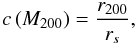 (40)while the
characteristic density is given by
(40)while the
characteristic density is given by  (41)Therefore, it
remains to specify the concentration parameter as a function of the halo mass, which we
have labeled M200 above to remind that it corresponds to the
mass defined by the nonlinear density contrast δ = 200. Although we shall
also consider fits to numerical simulations that have already been proposed in the
literature, we shall find in Sect. 5 below that a
better match to numerical simulations for the density power spectrum (especially in the
high-k tail) is obtained with the following prescription,
(41)Therefore, it
remains to specify the concentration parameter as a function of the halo mass, which we
have labeled M200 above to remind that it corresponds to the
mass defined by the nonlinear density contrast δ = 200. Although we shall
also consider fits to numerical simulations that have already been proposed in the
literature, we shall find in Sect. 5 below that a
better match to numerical simulations for the density power spectrum (especially in the
high-k tail) is obtained with the following prescription,  (42)which is
intermediate between the behaviors found in Dolag et al.
(2004) and Duffy et al. (2008). However,
this should not be trusted beyond the range studied in this paper
(z ≤ 3).
(42)which is
intermediate between the behaviors found in Dolag et al.
(2004) and Duffy et al. (2008). However,
this should not be trusted beyond the range studied in this paper
(z ≤ 3).
Since we obtain Eq. (42) from a comparison with the density power spectrum measured in simulations, it can be understood as an “effective” concentration parameter that also includes the mean effect of halo substructures. Although it is possible to build more sophisticated halo models that explicitly describe substructures (Giocoli et al. 2010), we do not investigate such refinements here. In the same spirit, it could be possible to include the mean effect of baryons on the total matter profile of the halos through such an “effective” concentration parameter (or another choice for the shape of the halo profile than the NFW formula (39)). However, this is also beyond the scope of the present study, and we leave such investigations to future works. In any case, it is clear that any modeling of halo profiles (either at an “effective” level or through detailed explicit models) can be incorporated in the framework we describe in this paper. In particular, this could improve the accuracy at high k as simulations probe smaller scales and provide tighter (and more robust) constraints on halo properties.
For practical purposes it is convenient to use halo profiles that have an explicit
expression for the Fourier transform defined in Eq. (31), especially if one is interested in high
wavenumbers k where the integrand shows fast oscillations. Let us
recall that for the NFW profile (39) one
has (Scoccimarro et al. 2001)
![Mathematical equation: \begin{eqnarray} \tu_M(k) & = & \left[ \ln(1+c) - \frac{c}{1+c} \right]^{-1} \Biggl \{ \frac{-\sin\left(ckr_s\right)}{(1+c)kr_s} \nonumber \\ && + \cos\left(kr_s\right) \bigl[\Ci\left[(1+c)kr_s\right] - \Ci\left(kr_s\right) \bigl]\nonumber\\ && + \sin\left(kr_s\right) \bigl[ \Si\left[(1+c)kr_s\right] - \Si\left(kr_s\right) \bigl] \Biggl\}, \end{eqnarray}](/articles/aa/full_html/2011/03/aa15685-10/aa15685-10-eq206.png) (43)where
(43)where
 and
and
 are the Cosine and Sine
integrals (Abramowitz & Stegun 1970).
are the Cosine and Sine
integrals (Abramowitz & Stegun 1970).
4. N-body simulations
In this section we describe the details of our N-body simulations, and we show the results of some tests of their possible systematic errors.
4.1. Set up
We adopt a flat ΛCDM model with cosmological parameters (Ωm,Ωb,h,σ8,ns) = (0.279,0.046035,0.701,0.817,0.96), which is consistent with 5 year observation of WMAP (Komatsu et al. 2009). We use a publicly available code, CAMB (Lewis et al. 2000), to compute the linear power spectrum. All the initial conditions for the simulations are created by adding displacements to particles put on a regular lattice by second-order Lagrangian perturbation theory (Scoccimarro 1998; Crocce et al. 2006) at z = 99, and evolved by a publicly available Tree Particle-Mesh code, GADGET2 (Springel 2005). We employ N = 20483 particles in four periodic boxes with different box sizes (Lbox = 512,1024,2048 and 4096 h-1 Mpc). We call these runs as L9-N11, L10-N11, L11-N11 and L12-N11, respectively. The softening lengths for the tree force are set to be 5% of the mean inter-particle distance.
In addition to the four main simulations, we run five smaller simulations (L9-N8, L9-N9, L9-N10, L10-N9 and L11-N10) for convergence tests. The box sizes and number of particles of these simulations are summarized in Table 1.
List of N-body simulations presented in this paper.
4.2. Measuring power spectrum and two-point correlation function
We basically follow the ordinary FFT method to measure both the power spectrum and the
two-point correlation function. Before assigning particles to the mesh, however, we fold
the particle distribution into a smaller box to avoid the systematic error caused by the
assignment on a finite number of grid points, which is important on small scales near the
grid interval (see Colombi et al. 2009, for a
similar discussion). Namely, we perform the following operation to the particle position,
x: 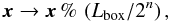 (44)where the operation,
a % b, gives the reminder of the division
of a by b, and we vary the integer n
from 0 to 6. After that, we assign particles on the 20483 grid points of the
folded small box with side length
of Lbox/2n using the CIC
algorithm (Hockney & Eastwood 1981). We
then Fourier transform the density contrast and take the average of
(44)where the operation,
a % b, gives the reminder of the division
of a by b, and we vary the integer n
from 0 to 6. After that, we assign particles on the 20483 grid points of the
folded small box with side length
of Lbox/2n using the CIC
algorithm (Hockney & Eastwood 1981). We
then Fourier transform the density contrast and take the average of
 within k-bins to obtain the power spectrum. The binning is chosen to be
logarithmic on small scale with 20 bins per decade
(k > 0.3 h Mpc-1), but we adopt
a linear binning with the interval
Δk = 0.005 h Mpc-1 on large scale
(k < 0.3 h Mpc-1) to see the
feature of BAOs more clearly. While the folding procedure makes the systematic effect
caused by assignment smaller, it reduces the number of available modes. We choose the
value of n for the folding depending on the wavenumber so that the number
of modes is large enough. We plot in Fig. 7 the
resulting statistical error (1-σ level) estimated from
within k-bins to obtain the power spectrum. The binning is chosen to be
logarithmic on small scale with 20 bins per decade
(k > 0.3 h Mpc-1), but we adopt
a linear binning with the interval
Δk = 0.005 h Mpc-1 on large scale
(k < 0.3 h Mpc-1) to see the
feature of BAOs more clearly. While the folding procedure makes the systematic effect
caused by assignment smaller, it reduces the number of available modes. We choose the
value of n for the folding depending on the wavenumber so that the number
of modes is large enough. We plot in Fig. 7 the
resulting statistical error (1-σ level) estimated from  (45)where
Nmode(k) denotes the number of independent
mode in that bin. This is exact when
(45)where
Nmode(k) denotes the number of independent
mode in that bin. This is exact when  is Gaussian (Feldman et al. 1994), and this can be shown to remain a
good estimate in the current situation (see e.g., Takahashi et al. 2009). One may notice a dip at
k ~ 0.3 h Mpc-1. This
corresponds to the change of binning from linear to logarithmic. Another feature is a
characteristic zig-zag pattern on smaller scale. This pattern corresponds to the change in
the value of n used in the folding. Even after reducing the number of
available modes by folding, however, we keep enough Fourier modes to achieve accuracy of
~ sub-percent level on small scale
is Gaussian (Feldman et al. 1994), and this can be shown to remain a
good estimate in the current situation (see e.g., Takahashi et al. 2009). One may notice a dip at
k ~ 0.3 h Mpc-1. This
corresponds to the change of binning from linear to logarithmic. Another feature is a
characteristic zig-zag pattern on smaller scale. This pattern corresponds to the change in
the value of n used in the folding. Even after reducing the number of
available modes by folding, however, we keep enough Fourier modes to achieve accuracy of
~ sub-percent level on small scale  .
.
The two-point correlation function is measured in a similar manner. We simply perform an
inverse FFT to the three dimensional power spectrum calculated on grid points. We estimate
the statistical error using the formula:  (46)where the
quantity j0 is the spherical Bessel function of the first
kind. We use the power spectrum measured from the same simulation in the integrand for
consistency, see Taruya et al. (2009) for more
details.
(46)where the
quantity j0 is the spherical Bessel function of the first
kind. We use the power spectrum measured from the same simulation in the integrand for
consistency, see Taruya et al. (2009) for more
details.
4.3. Convergence tests
One may naively think that one can model the power spectrum by combining simulations with different box sizes. However, it is not trivial to determine which simulation gives the best measurement on a given scale. The simulation in a larger volume lacks the power on small scale, while that in a smaller box does so on large scale.
A characteristic wavenumber for the finite box size is given by 2π/Lbox, the fundamental mode. For the finiteness of mass/force resolution, one may define two important wavenumbers. First, the initial density fluctuation cannot be input on scales smaller than the mean inter-particle distance (2π/Lbox × N1/3 in wavenumber). Second, the force calculation is not accurate below the softening scale. This wavenumber is given by 2π/Lbox × N1/3 × 20 for our simulations (i.e., 5% of the mean inter-particle distance). One can basically trust the simulation results from the fundamental mode to the inter-particle distance, or at most to the softening scale. These wavenumbers are shown in the left panel of Fig. 2 for the four main simulations.
 |
Fig. 2 Wavenumber ranges covered by our N-body simulations, from the fundamental mode (left edge) to the mean inter-particle scale (solid right edge) and to the softening scale (dashed right edge). Left: the four main simulations, middle: simulations used in Test 1, right: simulations used in Test 2. |
 |
Fig. 3 The ratio of the power spectrum to the highest resolution run, L9-N11. The three lines correspond to L9-N10, L9-N9 and L9-N8 from top to bottom. Left: z = 3, middle: z = 1, right: z = 0.35. |
After nonlinear evolution, however, the initial small systematic error on one scale may propagate to different scales due to the coupling between different modes. This makes the situation complicated. To separate the two systematic effects caused by the finiteness of mass/force resolution and simulated volume, we perform two tests using additional simulations in this subsection. We will show that both finiteness effects lead to a lack of power on certain scales. We especially focus on the scales where these effects are more than 1%, and avoid to use the data points on these scales in later discussions.
4.3.1. Test 1: finite mass/force resolution
We first examine the effect of the finiteness of the mass/force resolution. We use L9-N8, L9-N9, L9-N10 and L9-N11 for this test (see Table 1). These simulations have the same volume but different number of particles, so that we can see the systematic effect purely from the finiteness of the resolution (see the middle panel of Fig. 2). We set the same random linear density field in creating the initial conditions of the four simulations to make the comparison clearer. Since the three additional simulations, L9-N8, L9-N9 and L9-N10, have the same resolution as L12-N11, L11-N11 and L10-N11, respectively, we can assess the impact of the systematic effect for the “main” simulations by this test.
The results are shown in Fig. 3. We plot the ratio of the power spectrum measured from the three lower resolution runs to that from the highest resolution one (i.e., L9-N11). One can clearly see that all curves blow up at large wavenumbers. This corresponds to the scale where the shot noise contribution becomes important. In addition to this feature, the curves show a lack of power on intermediate scales, which is more important for lower resolution runs at higher redshifts. We can interpret this as follows. At higher redshifts, the lack of power on around mean inter-particle scale survives. But the power generated by the pure nonlinear growth gradually dominates over the initial power and the difference between the four runs become smaller at lower redshifts.
We also test the effect of finite resolution on the two-point correlation function. Similar trends can be seen in Fig. 4 for the two-point correlation function.
4.3.2. Test 2: finite box size
We next discuss the effect of the finiteness of the simulated volume. We use L9-N8, L10-N9, L11-N10 and L12-N11 for this test (see Table 1). These runs have the same mass/force resolution but different box size (see the right panel of Fig. 2). Again, since the three smaller simulations have the same volume as the main runs, L9-N11, L10-N11 and L11-N11, we can test the possible systematics of these main simulations.
We show the results in Fig. 5. In contrast to the test for the finite resolution, the data points seem noisy. This is because we cannot set the same random realization of the linear density field for simulations with different box sizes. When one sees the result of L9-N8, the systematic effect is prominent at 0.3 ~ 2 h Mpc-1, and is growing with time. This is contrary to what we see in the finite resolution test, which as we showed was decaying. This growing nature of the systematics suggests that the effect comes from the mode coupling of large-scale modes. The systematic effect is not important (i.e., below 1% level) for the rest of the simulations.
 |
Fig. 5 The ratio of the power spectrum to the largest volume run, L12-N11. The three symbols correspond to L11-N10 (triangles), L10-N9 (circles) and L9-N8 (diamonds). Left: z = 3, middle: z = 1, right: z = 0.35. |
We test the convergence of the two-point correlation function which is shown in Fig. 6. Unfortunately, however, we cannot determine a strict range of the trustable scales due to large statistical error. Since the two-point correlation function is a weighted sum of the power spectrum over all scales, a large error bar at a certain wavenumber may propagate to the two-point correlation function over a wide range of scales. Furthermore, the two-point correlation function is not positive definite unlike the power spectrum. Thus, the size of its fractional error can be very large on scales where the two-point correlation function is close to zero. Finally, we cannot control the size of error bars by changing the width of the bins, since it does not explicitly depend on this width [see Eq. (46)].
The ratio of the two-point correlation function on scales above ≳5 h-1 Mpc seems consistent with unity at all the three redshifts. As seen in Fig. 6, the finite resolution effect is important below ≲5 h-1 Mpc for L9-N8. This prevents us from a clear test for the finite box size since the four simulations used in this test have the same resolution as L9-N8. We conclude here that we do not find any clear evidence of systematic error on the two-point correlation function arising from the finiteness of volume, and we will determine which simulation to use following only the resolution test. We leave more complete tests for the finite volume to future works.
 |
Fig. 7 1-σ statistical error of the power spectrum (fractional) estimated from Eq. (45) for L9-N11, L10-N11, L11-N11 and L12-N11 (from top to bottom). |
 |
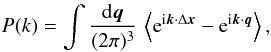
Fig. 8 The probability F2H(1/k) that a Lagrangian pair of distance q = 1/k belongs to different halos, from Eq. (21). We show our results for z = 0.35, 1, and 3. |
5. Comparison with numerical simulations
We first show in Fig. 8 the
quantity F2H(1/k), which is defined by
Eq. (21) and enters the 2-halo term (27), at redshifts z = 0.35, 1,
and 3. At fixed comoving scale, q = 1/k, it decreases at
lower redshift, since the probability F1H for a Lagrangian pair
of distance q to belong to the same collapsed halo grows with time, as
larger scales turn nonlinear, and
F2H = 1 − F1H. We can note that it
decreases very slowly at high k. In fact, since we consider an initial
power spectrum with a primordial slope
ns = 0.96 that is smaller than unity, the rms
linear density contrast σ(q) of Eq. (10) does not diverge to infinity as
q → 0 but goes to a finite asymptote. This implies that the
probability F2H(1/k) does not go to zero at
high k (i.e. on small scales), but reaches the nonzero asymptote
 . Although this value is
unlikely to be exact, because of the approximations involved in the derivation
of F2H(q), it is possible that for such power
spectra without significant power on small scales there always remains some fraction of
matter which has never experienced shell crossing and remains described by the single-stream
fluid approximation. Even though this is an interesting point from a theoretical
perspective, regarding the dynamical properties of the system, this is beyond the subject of
the present work and it plays no role for our purposes, since at high k the
power spectrum is clearly dominated by the 1-halo term, as we shall check in Fig. 9 below. On the other hand, we can see that if we require a
high accuracy, the deviation of F2H from unity at
k ~ 0.3 h Mpc-1 for
z = 1 cannot be completely neglected and has some effect on the 2-halo
term (27).
. Although this value is
unlikely to be exact, because of the approximations involved in the derivation
of F2H(q), it is possible that for such power
spectra without significant power on small scales there always remains some fraction of
matter which has never experienced shell crossing and remains described by the single-stream
fluid approximation. Even though this is an interesting point from a theoretical
perspective, regarding the dynamical properties of the system, this is beyond the subject of
the present work and it plays no role for our purposes, since at high k the
power spectrum is clearly dominated by the 1-halo term, as we shall check in Fig. 9 below. On the other hand, we can see that if we require a
high accuracy, the deviation of F2H from unity at
k ~ 0.3 h Mpc-1 for
z = 1 cannot be completely neglected and has some effect on the 2-halo
term (27).
We now compare our model for the density power spectrum, that combines a systematic
perturbative approach with a phenomenological halo model, with results obtained from
numerical simulations. We show in Fig. 9 the power per
logarithmic interval of k, defined as  (47)for the three
redshifts z = 0.35, 1, and 3. The sudden rise of the
N-body results at very high k (which is more apparent in
the right panel at z = 3) is due to the finite resolution and shot noise,
see Sect. 4. This marks the highest wavenumber where
we can compare the simulations with our theoretical models.
(47)for the three
redshifts z = 0.35, 1, and 3. The sudden rise of the
N-body results at very high k (which is more apparent in
the right panel at z = 3) is due to the finite resolution and shot noise,
see Sect. 4. This marks the highest wavenumber where
we can compare the simulations with our theoretical models.
 |
Fig. 9 The power per logarithmic interval of k, as defined in Eq. (47), at redshifts
z = 0.35, 1, and 3. The symbols are the results from the numerical
simulations described in Sect. 4. The black
solid line is the linear power spectrum, |


 |
Fig. 10 The ratio of the nonlinear power spectrum P(k) to a smooth linear power spectrum PLs without acoustic baryonic oscillations, from Eisenstein & Hu (1999). The points with error bars are the results from N-body simulations. The black solid line PL is the linear power spectrum, and the upper blue dashed line P1loop is the prediction of standard perturbation theory up to one-loop order. The green solid line P is the full nonlinear power spectrum, from Eq. (22), whereas the lower blue dotted line Ppert is the perturbative part. The magenta dot-dashed line PS is the fit to simulations from Smith et al. (2003) (which was not specifically designed to reproduce the baryon oscillations). |
As discussed in Sect. 3.1, we can check that the
2-halo term  remains well-behaved
at high k and is subdominant with respect to the 1-halo term
remains well-behaved
at high k and is subdominant with respect to the 1-halo term
 . It falls somewhat
below the linear power
. It falls somewhat
below the linear power  , contrary to
the one-loop resummation of
, contrary to
the one-loop resummation of  given by the
direct steepest-descent scheme, which becomes very close to
as seen in Valageas (2007a), because of the
prefactor F2H(1/k) in Eq. (27).
given by the
direct steepest-descent scheme, which becomes very close to
as seen in Valageas (2007a), because of the
prefactor F2H(1/k) in Eq. (27).
In agreement with the discussion of Sect. 2.3, we can also check that the 1-halo term shows a fast decline at low k. At high k we can see that it is possible to reach a good agreement with the numerical simulations by using an appropriate prescription for the concentration parameter c(M), such as the one given in Eq. (42) and represented by the green solid line. The formula given in Eq. (42) is obtained by looking for values of the free parameters (the normalization and the two exponents) that provide a reasonable match with the power spectrum measured in the simulations at high k (looking among a few values close to the fits already proposed in the literature). Nevertheless, it is interesting to note that using fits for c(M) proposed in previous analysis of the halo profiles formed in numerical simulations, one obtains predictions that are either larger (Dolag et al. 2004) or smaller (Duffy et al. 2008) than the one associated with Eq. (42). This shows that the nonlinear power spectrum is fully consistent in this range with a simple halo model, such as (35), and with the properties of halos seen in numerical simulations. This also gives an estimate of the dependence of the power spectrum on the prescription used for c(M). In agreement with previous works (Huffenberger & Seljak 2003; Giocoli et al. 2010), we recover the fact that the nonlinear power Δ2(k) is larger and steeper at high k for concentration relations c(M) that have a larger normalization and a steeper dependence on M. A nice feature is that the nonlinear power is largely independent of the details of the halo model up to Δ2 < 100, so that models such as the one studied in this article remain quite predictive. Even at higher k, we can see that up to Δ2 < 103, or k < 100 h Mpc-1, using any of these prescriptions for c(M) provides a reasonable estimate of the power spectrum and even fares better than the direct fit to P(k) that was obtained from older simulations (Smith et al. 2003). This suggests that models based on phenomenological ingredients such as the halo model may prove more robust than direct fits to numerical results. However, our model for P(k) should not be trusted beyond the domain where it has been checked, that is k ≤ 100 h Mpc-1 and z ≤ 3.
In order to obtain predictions at much higher redshifts and wavenumbers, one should use a prescription for c(M) that is based on some physical arguments rather than simple fits such as Eq. (42). This would probably lead to a loss of accuracy in the range tested in Fig. 9, as compared with the use of Eq. (42), but this is likely to be more robust as we extrapolate to other regimes. However, we shall not investigate the building of physical models for c(M) in this article, as this is a topic by itself.
We can see in Fig. 9 that the full nonlinear power spectrum (22) obtained by our approach, combining a perturbative expansion with a phenomenological halo model, is able to reproduce the results measured in numerical simulations, up to a reasonable accuracy. Let us point out that the perturbative part, Ppert(k), which dominates on large scales, contains no free parameter, since it is given by a systematic perturbation theory. The 1-halo contribution that dominates on small scales clearly contains some parameters, through the choice of the halo mass function and halo density profile. However, the mass function and the shape of the halo profile are already set by other measures from numerical simulations, so that the main free parameter is the concentration c(M), which is not as well constrained. However, as seen in Fig. 9, this uncertainty only affects the very high-k tail. Moreover, even in this region the resulting model is competitive with direct fits to the power spectrum measured in older simulations. Therefore, models such as the ones developed in this article should prove useful to obtain reliable predictions for P(k). Another advantage of such models, as compared with simpler fitting formulas, is that they should be quite accurate on large scales since they are consistent with perturbation theory, up to the order of truncation of the computation.
Thus, we plot in Fig. 10 the ratio of the power
spectrum to a “no-wiggle” linear power
spectrum PLs(k) which does
not include baryonic acoustic oscillations, in order to see more clearly the
low-k behavior. We can check that in this range our model, based on the
direct steepest-descent resummation, shows a good match with the numerical simulations. As
could be expected, it fares better than a direct fit from Smith et al. (2003) which was not designed to model this range with a high
accuracy (but still remains surprisingly good). Furthermore, the use of the direct
steepest-descent resummation proves to provide significantly more accurate results than the
standard perturbation theory, truncated at one-loop order, given by the well-known
expressions  (48)where formulas for the
terms P22 and P31 may be found for
instance in Bernardeau et al. (2002). Let us recall
here that the term Ppert(k) given by this
direct steepest-descent scheme contains no free parameter, nor any interpolation procedure,
and is consistent with standard perturbation theory up to one-loop order (i.e. the
difference between P1loop and Ppert
is due to the partial resummation of higher order terms). We can see in the left panel, at
z = 0.35, that around
k ~ 0.14 h Mpc-1 the
curve Ppert is slightly above the full nonlinear power
spectrum P. This is due to the
prefactor F2H(1/k) in Eq. (27), which is slightly below unity. However,
this is only a very small effect on these scales. On the other hand, at
higher k (e.g.,
k > 0.26 h Mpc-1 at
z = 0.35) the nonlinear power spectrum rises above
Ppert and keeps growing,
while Ppert remains close to PL at
high k as seen in Fig. 9. This is
due to the 1-halo contribution, which starts being non-negligible. However, on these scales
the dependence on the details of the halo model is extremely weak. Indeed, the three green
curves plotted in Fig. 9, associated with the
prescription (42) for the
concentration c(M) and the two fits given by Dolag et al. (2004) and Duffy et al. (2008), are also plotted in Fig. 10. However, they almost exactly fall on top of each other and cannot be
distinguished in the figure.
(48)where formulas for the
terms P22 and P31 may be found for
instance in Bernardeau et al. (2002). Let us recall
here that the term Ppert(k) given by this
direct steepest-descent scheme contains no free parameter, nor any interpolation procedure,
and is consistent with standard perturbation theory up to one-loop order (i.e. the
difference between P1loop and Ppert
is due to the partial resummation of higher order terms). We can see in the left panel, at
z = 0.35, that around
k ~ 0.14 h Mpc-1 the
curve Ppert is slightly above the full nonlinear power
spectrum P. This is due to the
prefactor F2H(1/k) in Eq. (27), which is slightly below unity. However,
this is only a very small effect on these scales. On the other hand, at
higher k (e.g.,
k > 0.26 h Mpc-1 at
z = 0.35) the nonlinear power spectrum rises above
Ppert and keeps growing,
while Ppert remains close to PL at
high k as seen in Fig. 9. This is
due to the 1-halo contribution, which starts being non-negligible. However, on these scales
the dependence on the details of the halo model is extremely weak. Indeed, the three green
curves plotted in Fig. 9, associated with the
prescription (42) for the
concentration c(M) and the two fits given by Dolag et al. (2004) and Duffy et al. (2008), are also plotted in Fig. 10. However, they almost exactly fall on top of each other and cannot be
distinguished in the figure.
Thus, Figs. 9 and 10 show that by combining perturbation theories and halo models it is possible to obtain a good model for the nonlinear density power spectrum, both on quasi-linear and highly nonlinear scales. However, we can see in Fig. 9 that in the intermediate regime, where Δ2 ~ 5, our predictions fall below the N-body results. This is also apparent in the high-k parts of Fig. 10, where the full nonlinear prediction P(k) starts to grow more slowly than the power measured in the numerical simulations. This regime corresponds to the transition between the 2-halo and 1-halo contributions (see Fig. 9) and as such it is at the limit of validity of the approximations used for both terms.
On the perturbative side, that is the 2-halo term, the discrepancy can be due to the truncation at one-loop order of the perturbative term. Indeed, we can expect that by going to higher orders we can extend the range of validity of the the perturbative term Ppert and push the downturn shown by the blue dotted curve in Fig. 10 to higher k. Within such resummation schemes this means that we include all diagrams up to n loops, and partial resummations for higher order terms. We can note that the discrepancy looks somewhat more severe at z = 3 in Fig. 9. More precisely, the range of k where there is a noticeable mismatch before the 1-halo term becomes dominant (larger than PL) is somewhat more extended than at z = 0.35. This agrees with the results of Valageas (2010a), where it was found (within the Zeldovich framework) that the scope of perturbation theory is somewhat greater at higher redshift for CDM power spectra, in the sense that the range where higher order perturbative terms are important (i.e. larger than the non-perturbative correction associated with shell crossing effects) is wider and that the perturbative expansion makes sense up to higher orders. However, we shall not try to go beyond one-loop order in this paper and we leave such a task to future works.
On the non-perturbative side, it is clear that by definition halo models are only phenomenological models and do not provide a systematic tool. Even if we admit that it makes sense to “recognize” halos in the density field (even though this is a descriptive tool rather than a direct ingredient of the equations of motion), it is clear that realistic halos are not spherical nor fully virialized. In particular, apart from the inaccuracies introduced by the spherical approximations, outer halo radii are not fully virialized and particles do not instantly loose all memory of their initial conditions, so that the average in Eq. (33) is only approximate. As we have discussed in Sect. 2.3, such approximations also prevent us from exactly satisfying momentum conservation. Since these effects mostly apply to the outer parts of the halos they can be expected to have an impact on the moderately low-k part of the power spectrum, that is the transition region. Another effect that is likely to play a role is the truncation of the halo profiles at the radius r200. This may be investigated in a rather straightforward manner by studying the change in P(k) as we modify this density threshold, and we shall consider in Sect. 6.1 below the results obtained for δ = 50.
On a more fundamental level, since the splitting between 2-halo and 1-halo contributions is necessarily approximate (it cannot be derived in a systematic fashion from the equations of motion and always involves some approximations, at least within analytical frameworks) it is not surprising that the match is not perfect, especially in the transition range.
Another approximation used in this work is the assumption of smooth halos, defined by the regular profile (39). As noticed in Sect. 3.2, it is possible to extend the halo model by including substructures (Giocoli et al. 2010), however this only has an effect on the very high-k tail of the power spectrum (as could be expected since these are small-scale modifications). We do not investigate such modifications in this work, as the agreement we obtain with numerical simulations is already reasonably good on these scales and we prefer not to introduce additional parameters. These effects are also degenerate with the mean concentration relation c(M), as seen in Fig. 9 by the comparison between the dashed and dotted green curves, associated with different prescriptions from Dolag et al. (2004) and Duffy et al. (2008). In particular, as pointed out in Sect. 3.2, the prescription (42) that we have obtained by requiring a good match at high k can also be seen as an effective model, that describes the combined effects of both the concentration of the mean radial profile and the presence of small substructures. At some stage, if one wants to build a model where the halo properties are independently obtained from the measure of individual halos in N-body simulations, so that c(M) can no longer be tuned, it may nevertheless prove necessary to explicitly include such effects.
6. Dependence on various ingredients of the model
We now investigate the impact of various ingredients of the model on the predictions obtained for the density power spectrum.
6.1. Halos defined by δ = 50
As we have discussed in the previous section, the lack of power on intermediate scales seen in Fig. 9, around the transition between the 2-halo and 1-halo terms, may be due in part to the truncation of the halo profiles at the radius r200. Indeed, realistic halos extend to larger radii, which should generate some extra power on large scales. In order to take into account such outer radii, while keeping the mass M that enters the definition of the halo mass function as the halo mass within the truncation radius (so as to avoid overcounting and violations of mass normalizations), we consider defining halos by a smaller nonlinear density contrast, such as δ = 50. This lower threshold means that we include outer shells (as compared with the case δ = 200), while halos still remain well separated from the background.
For the halo mass function we still use the scaling function (38), but the linear density contrast is now δL = ℱ-1(50), which gives for instance δL ≃ 1.50 at z = 1. This automatically satisfies the normalization (15) as well as the large-mass tail (14). It was shown in Valageas (2009a) that this recipe provides a reasonable match to numerical simulations (but not as good as for δ = 200) for halos defined by a density threshold δ = 100, and we shall assume that it still provides a reasonable model for δ = 50. This should be sufficient for our purposes, as the 1-halo term needed for the density power spectrum only depends on integrals over the halo mass function and we have seen that both the normalization and the large-mass tail are correctly reproduced.
We still use the NFW profile of Eq. (39),
but we now need to obtain the scale radius rs
in terms of r50. To do so, we now define the concentration
parameter as  (49)and the halo
characteristic density now reads as
(49)and the halo
characteristic density now reads as  (50)We again look for
a prescription for c(M50) of the form of
Eq. (42), and we find in Fig. 11 below that a reasonable agreement with the numerical
simulations can be achieved by using
(50)We again look for
a prescription for c(M50) of the form of
Eq. (42), and we find in Fig. 11 below that a reasonable agreement with the numerical
simulations can be achieved by using  (51)This is mostly
set by the behavior of the power spectrum at high k, where
Δ2 > 100, as seen in Fig. 9 from
the comparison between various models for c(M) for halos
defined by δ = 200. Thus, the properties of the density power spectrum on
large scales, where Δ2 < 10, are almost independent of the choice of
parameters in Eq. (51) (restricted to a
reasonable range).
(51)This is mostly
set by the behavior of the power spectrum at high k, where
Δ2 > 100, as seen in Fig. 9 from
the comparison between various models for c(M) for halos
defined by δ = 200. Thus, the properties of the density power spectrum on
large scales, where Δ2 < 10, are almost independent of the choice of
parameters in Eq. (51) (restricted to a
reasonable range).
 |
Fig. 11 The power per logarithmic interval of k, as in Fig. 9, but for halos that are defined either by a density contrast δ = 200 (solid curves, identical to those of Fig. 9), or by δ = 50 (dot-dashed curves). Both the 1-halo contribution Δ1H and the full nonlinear power spectrum Δ2 are shown. |
We compare in Fig. 11 the power spectra obtained on nonlinear scales by using halos defined either by δ = 200 or δ = 50 (while the perturbative term Ppert(k) is not modified). As expected, truncating halo profiles at a larger radius yields some extra power at large k and improves somewhat the agreement with numerical simulations in the intermediate range, where Δ2 ~ 5. However, the change is quite small and the match to the N-body results is not perfect yet. In fact, at redshift z = 0.35, we obtain a smaller power spectrum around Δ2 ~ 100 by using halos defined by δ = 50. However, one may modify this by using a different concentration relation c(M50) at that redshift. In any case, these results suggest that the truncation at r200 is not the unique reason for the discrepancy between the model and N-body simulations in this transitory range, and as explained in Sect. 5 another possible source of inaccuracy is the partial resummation of high-order terms in the perturbative term Ppert.
Next, we compare in Fig. 12 the power spectra obtained on quasi-linear scales. We can see that on these very large scales, k < 0.3 h Mpc-1, the modification of the 1-halo term has a very weak effect. However, it improves somewhat the agreement with the simulations at low redshift, z = 1 (at k ~ 0.3 h Mpc-1, as the gap below the N-body results in the intermediate range is repelled to slightly higher k), although it leads to a slight overestimate for P(k) at z = 0.35. On the other hand, it appears to make almost no change over these scales at higher redshift, z = 3. In agreement with the discussion in Sect. 5 and with Valageas (2010a), this expresses the fact that for CDM power spectra the scope of perturbative expansions is somewhat broader at higher z, in the sense that the range of k where higher order terms play a role is wider. This corresponds to the interval [ k1loop,ks.c. ] where terms beyond linear order are already significant, as compared with the linear power PL, but still larger than the non-perturbative correction associated for instance with shell crossing effects.
 |
Fig. 12 The ratio of the nonlinear power spectrum P(k) to a smooth linear power spectrum PLs without acoustic baryonic oscillations, as in Fig. 12, for halos defined by δ = 200 (green solid curves, identical to those of Fig. 10), or by δ = 50 (red dot-dashed curves). |
That our results for the density power spectrum only show a very weak dependence on the details of the halo definition (by δ = 200 or 50) can actually be considered as a reassuring sign, rather than a problem in the attempt to improve the agreement with simulations. Indeed, if the splitting (22) and all subsequent computations were exact, halos would only appear as an intermediate tool and would disappear in the final result, since the matter density field is independent of how we split it over halos at later stages. Therefore, the final result for P(k) should not depend on the details of the definition of the halos. In practice, this cannot be the case because the splitting (22) itself is only approximate as long as we consider spherical halos, and the subsequent treatment of both 2-halo and 1-halo contributions involves some approximations, as in Eqs. (27) and (32). This leads to some artificial dependence on the details of the halo model, but as shown in Figs. 11 and 12 this effect is rather small and argues for the robustness of the model.
Therefore, Figs. 11 and 12 suggest that there is still room for systematic improvement, by including higher order terms in the perturbative contribution Ppert. However, this may come at the price of heavier and slower computations, which we do not investigate here. On the other hand, they show that predictions on large scales are largely independent of the details of the underlying halo model.
 |
Fig. 13 The ratio of the nonlinear power spectrum P(k) to
a “no-wiggle” linear power
spectrum PLs(k), as
in Fig. 10, at redshifts
z = 0.35, 1, and 3. The green solid lines correspond to our
fiducial model, with halos defined by a density contrast δ = 200,
and are identical to the green solid lines shown in Fig. 10, while the red dashed lines are obtained by setting to zero
the 1-halo counterterm |
6.2. Impact of the “1-halo” counterterm
We have seen in Sects. 5 and 6.1 that quantitative details of the 1-halo term can have some effect
on the high-k tail (the
concentration c(M) of the halo profiles) or on the
intermediate range where Δ2(k) ~ 5 (the truncation
radius of the halos). We investigate here the role of a more fundamental ingredient of the
1-halo contribution, namely the counterterm in Eq. (35). Thus, focusing on the case of halos
defined by the nonlinear density contrast δ = 200, we compare in
Fig. 13 the predictions of our fiducial model with
those that are obtained by setting to zero the 1-halo counterterm
of Eq. (35). Thus, we can see that, even though the
1-halo counterterm plays a negligible role at high k, it cannot be
discarded at low k if we require a high accuracy. As explained in
Sect. 2.3, this is also related to the fact that
this counterterm is required to obtain the k2 tail at
low k expected for the 1-halo contribution (if we do not insist on
momentum conservation). Discarding this counterterm leads to a nonzero asymptote at
low k for P1H(k), which
eventually dominates over the linear power spectrum, which roughly decreases as
PL(k) ~ k for CDM
cosmologies. On the scales probed in Fig. 13,
k ~ 0.2 h Mpc-1, we have not
entered yet the very low k regime where this would give rise to a
spurious divergence. However, we can clearly see the spurious extra power that would be
generated by the lack of this counterterm. Note that on these scales there are no fitting
parameters that could be tuned to compensate for this extra power. Indeed, the details of
the halo model, such as the concentration c(M) (see
Fig. 10), or the truncation radius of the profiles
(see Fig. 12), only have a weak impact in this
domain and could not balance this extra power. On the other hand, the 2-halo term is also
highly constrained, as the blue dashed and dotted curves in Fig. 10, associated with standard 1-loop perturbation theory and
steepest-descent resummation, give an estimate of the possible scatter between the
predictions that can be obtained from various perturbative schemes. This is most clearly
seen around the peak at
k ~ 0.13 h Mpc-1 for
z = 0.35 (as could be expected the extra power associated with such an
incorrect modelization of the 1-halo term grows at lower z as larger
halos form). By contrast, the reasonably good agreement with simulations obtained by our
complete model (solid lines) suggests that it does not miss important physical ingredients
(as discussed in Sect. 5 difficulties mostly arise
at higher k, associated with the transition between the 2-halo and 1-halo
contributions).
 |
Fig. 14 The ratio of the nonlinear power spectrum P(k) to a “no-wiggle” linear power spectrum PLs(k), as in Fig. 10, at redshifts z = 0.35, 1, and 3. The green solid lines “resum” correspond to our model as in Fig. 10, whereas the blue dashed lines correspond to the approximation P2H = PL (it cannot be distinguished from the linear power PL on these scales at z = 3). |
6.3. Benefit of higher order perturbative terms
Before we investigate other choices for the perturbative
term Ppert in the next sections, we first compare in
Figs. 14 and 15 our model with the more standard approach, where one simply uses the linear
power PL for the 2-halo contribution. Thus, we replace
Eq. (27) by the approximation
P2H(k) = PL(k),
while we keep the same 1-halo contribution (35), with its new counterterm that ensures a satisfactory behavior at
low k. In agreement with previous works, we can see in Fig. 14 that on the large scales associated with the baryon
acoustic oscillations the approximation
P2H(k) = PL(k)
is not sufficient to obtain a good match to the numerical simulations, contrary to the use
of the one-loop perturbative term Ppert(k)
obtained by the “steepest-descent” scheme recalled in Sect. 3.1. This means that on these scales the departure from the linear power is not
yet due to the non-perturbative contribution associated with the 1-halo term, but to
higher order perturbative terms. This agrees with the results of Valageas (2010a), based on the Zeldovich dynamics, which show that many
orders of perturbation theory are relevant before the power spectrum is dominated by the
non-perturbative contribution associated with shell crossing or halo formation (typically
one can go up to order  at
z = 0 and
at
z = 0 and  at
z = 3 for a ΛCDM cosmology, at least for this simpler case). This
motivates the use of perturbative approaches that include higher order contributions.
at
z = 3 for a ΛCDM cosmology, at least for this simpler case). This
motivates the use of perturbative approaches that include higher order contributions.
On smaller scales, shown in Fig. 15, the difference between our model for P2H(k) and the popular approximation P2H(k) = PL(k) is negligible. This agrees with Fig. 9, where we could see that at high k the one-loop resummed contribution to P2H(k) is near the linear power PL(k) and subdominant as compared with the 1-halo contribution.
 |
Fig. 15 The power per logarithmic interval of k, as in Fig. 9, at redshifts z = 0.35, 1, and 3. We plot the curves obtained with our model (green solid lines) and with the approximation P2H = PL (blue dashed lines), as in Fig. 14. |
6.4. Eulerian perturbation theories
We consider here two other choices for the perturbative term Ppert of the 2-halo contribution (27). A first choice is simply to use the standard perturbation theory and to write at one-loop order Ppert = P1loop(k), where P1loop(k) was given in Eq. (48). A second choice is to keep the diagrammatic expression given by the first line in Fig. 1, but to replace the external double lines by the Gaussian-decay response function (propagator) obtained by Crocce & Scoccimarro (2006b,a) instead of using the response function obtained by the steepest descent resummation scheme. This is not identical to the “RPT” resummation used in Crocce & Scoccimarro (2008), where the “bubble” in the upper right diagram of Fig. 1 is also replaced by resummed two-point correlations, obtained from this same nonlinear propagator (which corresponds to the partial resummation of further diagrams). Here we keep linear two-point correlation functions in this “bubble” to keep factorizable integrals, as in Eq. (A.29), since our goal is simply to estimate the dependence on the choice of resummation scheme. Moreover, it is interesting to evaluate various factorizable schemes of this kind as they allow faster computations. Two other differences with the prescription used in Crocce & Scoccimarro (2008) are the presence of the prefactor F2H(1/k) in Eq. (27), and the fact that we do not introduce an extra tuning in the decay of the response function by replacing the linear velocity dispersion σv, which governs its high-k cutoff, by a nonlinear velocity dispersion obtained from fits to the nonlinear power spectrum from numerical simulations. Indeed, one of the main points of our approach is precisely that the term Ppert(k) in the 2-halo contribution (27) should be obtained from systematic perturbation theories, to ensure a good accuracy and robustness for a variety of cosmologies, so that we avoid introducing fitting parameters in this factor. Then, these two alternatives, “standard perturbation theory” (SPT) and “Gaussian-like decaying response function” (DR), and the complete steepest-descent resummation used in the previous sections, agree with each other up to one-loop order.
 |
Fig. 16 The ratio of the nonlinear power spectrum P(k) to a “no-wiggle” linear power spectrum PLs(k), as in Fig. 10, at redshifts z = 0.35, 1, and 3. The red dashed lines “SPT” correspond to the use of 1-loop “Standard Perturbation Theory” for the term Ppert in the 2-halo contribution (27), whereas the blue solid lines “DR” correspond to the use of the “Decaying Response” function from Crocce & Scoccimarro (2006a) in the external double lines of the two upper diagrams of Fig. 1. The 1-halo term is the same as the one used in Sect. 5. |
We first show in Fig. 16 the power spectra obtained on large scales for redshifts z = 0.35,1, and 3. We plot the results obtained by using either the 1-loop “standard perturbation theory”, or the “decaying response” function from Crocce & Scoccimarro (2006a) in the external double lines of the two upper diagrams of Fig. 1, for the term Ppert in the 2-halo contribution (27). In both cases the 1-halo term is the same as the one used in Sect. 5, so that these curves only differ from those shown in Fig. 10 through the term Ppert. As was already noticed in Fig. 10, and in agreement with previous works (Crocce & Scoccimarro 2008; Taruya & Hiramatsu 2008; Carlson et al. 2009), the 1-loop standard perturbation theory overestimates the power on these scales, especially at low redshift. The dashed curves shown in Fig. 16 are not identical to those shown in Fig. 10 and in other works, because the perturbative term Ppert is multiplied by the prefactor F2H(1/k) in Eq. (27). Moreover, the results also include the (small) 1-halo contribution. However, on these scales the prefactor F2H(1/k) remains very close to unity (see Fig. 8) and it is not sufficient to significantly improve the agreement with the N-body results. The use of the “decaying response” function leads to results that are very close to those obtained with standard perturbation theory and also overestimates the power spectrum on these large scales. Using the full “renormalized perturbation theory” (RPT) described in Crocce & Scoccimarro (2008) leads to a smaller prediction for P(k). This can be understood from the fact that inserting the “decaying response” function into the bubble of the upper right diagram of Fig. 1, as in “RPT”, clearly suppresses the nonlinear power and explicit computations show that this yields a good match to results from simulations (Crocce & Scoccimarro 2008; Carlson et al. 2009).
 |
Fig. 17 The power per logarithmic interval of k, as in Fig. 9, at redshifts z = 0.35, 1, and 3. We plot the curves obtained using 1-loop “standard perturbation theory” (red dashed lines for the full nonlinear power Δ2, and lower red dotted lines for the associated 2-halo contribution) or the “decaying response” function from Crocce & Scoccimarro (2006a) (blue solid lines for the full nonlinear power Δ2, and lower blue dotted lines for the associated 2-halo contribution). Both the full and 2-halo power spectra obtained with “SPT” are larger than their “DR” counterparts. |
Next, we show in Fig. 17 the power per logarithmic interval of k, as in Fig. 9. We plot both the full nonlinear power Δ2, as in Fig. 16, and the 2-halo contribution, for the “SPT” and “DR” cases. As already pointed out in Sect. 3.1, we can see that standard perturbation theory fails at a qualitative level as the 2-halo contribution keeps growing at high k and becomes very large, whereas the term Ppert being associated with particle pairs that have not collapsed within a single object it should remain near PL at most. Moreover, this spurious growth is not suppressed by the prefactor F2H(1/k), which does not decrease sufficiently fast at high k, as seen in Fig. 8. Even though this 2-halo contribution remains smaller than the 1-halo contribution on these scales, it leads to a significant extra power that worsens the agreement with the numerical simulations. As can be seen from Figs. 9 and 11, this extra power cannot be compensated by modifications to the underlying halo model (such as the concentration c(M) or the halo truncation radius), especially in the range 5 < Δ2 < 200 where the dependence on the details of the halo model is rather weak. Of course, this problem would become increasingly severe as one includes higher order terms that grow increasingly fast at high k (Bernardeau et al. 2002; Crocce & Scoccimarro 2006b). This means that standard perturbation theory cannot be used to build systematic models for the density power spectrum, such as those studied in this paper. As pointed out in Sect. 3.1, this provides a further motivation to investigate resummation schemes that would be better behaved.
We can see that using the “decaying response” function in the external double lines of Fig. 1 leads to a 2-halo contribution that remains small and close to the linear power spectrum at high k, as for the direct steepest-descent scheme used in Fig. 9. This shows again the benefit of using resummation schemes instead of standard perturbation theory to obtain a well-behaved perturbative term Ppert(k) that also agrees with standard perturbation theory up to the order of truncation. In fact, it happens that using this “decaying response” function yields a somewhat larger perturbative term than the one obtained in Sect. 5 on large scales, as seen in Fig. 16, and this extra power actually improves the agreement with the N-body results in the range where 1 < Δ2 < 100. Indeed, as discussed in Sect. 5, the implementation used in Fig. 9 underestimates the nonlinear power spectrum in this range, and the additional power due to the use of this “decaying response” function helps to bridge the gap. It actually provides a very good quantitative match, although at z = 3 we again underestimate somewhat the power spectrum in the transition range. Thus, for practical quantitative purposes this may provide a good variant of the model developed in this paper to compute the power spectrum, if one is interested in these transition scales. However, because on large scales this prescription actually gives a worse match to numerical simulations, as seen in Fig. 16, the better agreement on the transition scales is probably not more than a lucky coincidence. Thus, it is likely to compensate a meaningful lack of power (due to the various reasons discussed in Sect. 5, such as the neglect of some higher order perturbative terms or the limitations of the description in terms of spherical virialized halos) by an unrelated artificial overestimate.
6.5. Lagrangian perturbation theories
The Lagrangian re-interpretation of the halo model developed in this paper, leading to the expression (26) for the 2-halo contribution, would most naturally lead us to consider Lagrangian perturbation theories. It is possible to substitute such schemes into Eq. (26), which allows us to integrate in a self-consistent fashion over the q-dependent prefactor F2H(q). Unfortunately, this does not yield very successful results while leading to somewhat more complex expressions than those encountered in Eulerian frameworks. Therefore, in this section we illustrate the problems faced by current Lagrangian schemes by using the simpler expression (27), where the term F2H(q) has been factorized as the prefactor F2H(1/k). Thus, as for the Eulerian perturbation theories used in the previous sections, we only need the prediction for the resummed power Ppert(k) to compute the 2-halo contribution. This simplifies matters and only makes a negligible change on large scales where F2H ≃ 1.
We consider two schemes that are inspired by a Lagrangian framework. A first approach is
the one presented in Matsubara (2008), which for
our purposes amounts to expand P(k) after factorization
of a Gaussian damping term  (see also Crocce & Scoccimarro 2006b; Valageas 2010a),
where σv is the rms one-dimensional
linear displacement (or the rms one-dimensional linear velocity, up to a time-dependent
factor) given by
(see also Crocce & Scoccimarro 2006b; Valageas 2010a),
where σv is the rms one-dimensional
linear displacement (or the rms one-dimensional linear velocity, up to a time-dependent
factor) given by  (52)Thus, at 1-loop
order the density power spectrum reads as (Matsubara
2008)
(52)Thus, at 1-loop
order the density power spectrum reads as (Matsubara
2008)  (53)where
P22 and P31 are the 1-loop terms
obtained in the standard Eulerian perturbation theory, as in Eq. (48). Of course, Eq. (53) could be obtained at once by requiring
consistency with Eq. (48) at
order
(53)where
P22 and P31 are the 1-loop terms
obtained in the standard Eulerian perturbation theory, as in Eq. (48). Of course, Eq. (53) could be obtained at once by requiring
consistency with Eq. (48) at
order  . As discussed in
Valageas (2007b, 2008, 2010a), and as can be seen from the
computation of Lagrangian response functions (Bernardeau
& Valageas 2008, 2010a), the
prefactor
is associated with the coherent displacement of density structures by the long wavelengths
of the velocity field and should only appear in different-time quantities, under the form
. As discussed in
Valageas (2007b, 2008, 2010a), and as can be seen from the
computation of Lagrangian response functions (Bernardeau
& Valageas 2008, 2010a), the
prefactor
is associated with the coherent displacement of density structures by the long wavelengths
of the velocity field and should only appear in different-time quantities, under the form
 , where
Di is the linear growth factor at
redshift zi
and σv0 is the linear dispersion today,
where D(z = 0) = 1. Thus, looking for an expansion under
the form (53) leads to an artificially
strong Gaussian damping at high k, which has no physical meaning. In
order to remedy to this problem, which can also be seen as a consequence of the truncation
to a finite number of terms between the parenthesis in Eq. (53) (once we insist on looking for an expansion of this form), we note
that the nonlinear power spectrum generated by the Zeldovich dynamics (Zeldovich 1970) can also be written under this form,
, where
Di is the linear growth factor at
redshift zi
and σv0 is the linear dispersion today,
where D(z = 0) = 1. Thus, looking for an expansion under
the form (53) leads to an artificially
strong Gaussian damping at high k, which has no physical meaning. In
order to remedy to this problem, which can also be seen as a consequence of the truncation
to a finite number of terms between the parenthesis in Eq. (53) (once we insist on looking for an expansion of this form), we note
that the nonlinear power spectrum generated by the Zeldovich dynamics (Zeldovich 1970) can also be written under this form,
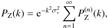 (54)where each term
 scales
as (PL)n. Moreover, both the
full nonlinear expression of the Zeldovich power spectrum,
PZ(k), (i.e. the resummation of the
series (54)), and the expression of the
terms (PL)n of all orders, are
explicitly known (Crocce & Scoccimarro
2006b; Valageas 2007b, 2010a). Then, a possible recipe is to use for the
nonlinear power spectrum (more precisely the perturbative
term Ppert) the “modified Zeldovich” expression
scales
as (PL)n. Moreover, both the
full nonlinear expression of the Zeldovich power spectrum,
PZ(k), (i.e. the resummation of the
series (54)), and the expression of the
terms (PL)n of all orders, are
explicitly known (Crocce & Scoccimarro
2006b; Valageas 2007b, 2010a). Then, a possible recipe is to use for the
nonlinear power spectrum (more precisely the perturbative
term Ppert) the “modified Zeldovich” expression
 where
P(n)(k) is the term of
order (PL)n in the expansion of
the form (54) for the gravitational power
spectrum, whence
where
P(n)(k) is the term of
order (PL)n in the expansion of
the form (54) for the gravitational power
spectrum, whence  from Eq. (53). In other words, we complete the expansion
(53) by substituting the terms obtained
for the Zeldovich power spectrum for all higher orders, which allows us to perform an
explicit resummation as in the second line of Eq. (56). This is clearly a systematic procedure, that can be pushed up to
any order, and agrees with standard perturbation theory up to the order of the
substitution. Since the resummed Zeldovich power spectrum no longer shows the spurious
Gaussian decay of Eq. (53) but a more
physical power-law decay (Taylor & Hamilton
1996; Valageas 2007b, 2010a), one may hope that this could improve the
agreement with results from numerical simulations.
from Eq. (53). In other words, we complete the expansion
(53) by substituting the terms obtained
for the Zeldovich power spectrum for all higher orders, which allows us to perform an
explicit resummation as in the second line of Eq. (56). This is clearly a systematic procedure, that can be pushed up to
any order, and agrees with standard perturbation theory up to the order of the
substitution. Since the resummed Zeldovich power spectrum no longer shows the spurious
Gaussian decay of Eq. (53) but a more
physical power-law decay (Taylor & Hamilton
1996; Valageas 2007b, 2010a), one may hope that this could improve the
agreement with results from numerical simulations.
We show in Fig. 18 the results we obtain using either Eq. (53) or (56), at redshifts z = 0.35, 1, and 3. As pointed out above, we can see that the Gaussian damping term of Eq. (53) leads to a fast decay for the nonlinear density power spectrum, which cannot be compensated by the 1-halo term. The “modified Zeldovich” expansion (56), which only implies a slower power-law decay at high k, fares better as the nonlinear power spectrum keeps growing on these scales. However, this is not sufficient to obtain a satisfactory match with the N-body results. Thus, the comparison with Fig. 10 shows that these Lagrangian-based expansions are not competitive with Eulerian schemes, and we do not investigate further these approaches in this paper. We note however that this is rather unfortunate, since in principles Lagrangian perturbation theories would seem better suited to compute the 2-halo term (26), and more importantly they should be better suited to computations in redshift space (Matsubara 2008). Therefore, it remains of interest to investigate whether other resummation schemes could be developed within the Lagrangian framework, but Fig. 18 suggests that some important new ingredients are required to make significant progress.
 |
Fig. 18 The ratio of the nonlinear power spectrum P(k) to a “no-wiggle” linear power spectrum PLs(k), as in Fig. 10, at redshifts z = 0.35, 1, and 3. The red dot-dashed lines “PMat” correspond to the use of the Lagrangian-based 1-loop expansion (53) for the term Ppert in the 2-halo contribution (27), whereas the blue solid lines “PmZ” correspond to the use of the “modified Zeldovich” expansion (56). The 1-halo term is the same as the one used in Sect. 5. |
 |
Fig. 19 The real-space two-point correlation function ξ(x), at redshifts z = 0.35, 1, and 3. The symbols are the results from the numerical simulations described in Sect. 4. The black dashed line is the linear correlation, ξL, and the blue dotted line which is somewhat below at low x is the 2-halo contribution ξ2H. The steep solid line xi1H is the 1-halo contribution, for the halo model described in Sect. 3.2. The green solid line is the full nonlinear correlation function, ξ = ξ2H + ξ1H. |
 |
Fig. 20 The real-space two-point correlation function ξ(x), at redshifts z = 0.35, 1, and 3, as in Fig. 19 but on larger scales. Since the 1-halo contribution is negligible on these scales we only show the linear correlation (black dashed line) and the full nonlinear correlation (green solid line). |
7. Real-space two-point correlation
Finally, we consider in this section the real-space two-point correlation function,
ξ( | x2 − x1 | ) = ⟨ δ(x1)δ(x2) ⟩ ,
that is predicted by our model. It is related to the Fourier-space power spectrum through
![Mathematical equation: \begin{eqnarray} \xi(x) & = & 4\pi \int_0^{\infty} \dd k \, k^2 P(k) \, \frac{\sin(kx)}{kx} \\[2mm] \label{xi-def} & = & \int_0^{\infty} \frac{\dd k}{k} \, \Delta^2(k) \, \frac{\sin(kx)}{kx}, \end{eqnarray}](/articles/aa/full_html/2011/03/aa15685-10/aa15685-10-eq345.png) so
that we obtain ξ(x) by integration over k
of the nonlinear power spectrum (22). In
particular, from the decomposition (22) we
can write the nonlinear correlation as the sum of 1-halo and 2-halo contributions,
so
that we obtain ξ(x) by integration over k
of the nonlinear power spectrum (22). In
particular, from the decomposition (22) we
can write the nonlinear correlation as the sum of 1-halo and 2-halo contributions,
 (59)which are the Fourier
transforms of the power spectra (23)
and (24).
(59)which are the Fourier
transforms of the power spectra (23)
and (24).
We show our results at redshifts z = 0.35, 1, and 3, in Figs. 19 and 20. Here we consider our fiducial model presented in Sects. 3 and 5, with the 2-halo perturbative term Ppert(k) given by the direct steepest-descent scheme detailed in Appendix A, and the 1-halo contribution obtained for halos defined by a density contrast δ = 200 and the mass-concentration relation (42).
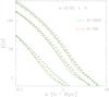 |
Fig. 21 The two-point correlation ξ(x), as in Fig. 19, but for halos that are defined either by a density contrast δ = 200 (solid curves, identical to those of Fig. 19), or by δ = 50 (dot-dashed curves). |
In agreement with our results for the power spectrum shown in Fig. 9, we can see in Fig. 19 that our model provides a good match to numerical simulations on both small and large scales. As is well known, on large scales the two-point correlation is governed by the 2-halo contribution ξ2H, whereas on small scales it is governed by the 1-halo contribution. As for the power spectrum, the transition scales where the 2-halo and 1-halo contributions are of the same order are more difficult to reproduce, and we again underestimate the power (here the real-space correlation) in this range. This is a direct consequence of the same feature observed in Fourier space in Fig. 9. In particular, we also find that the range and amplitude of this discrepancy is larger at z = 3 than at z = 0.35. Again, improving theoretical predictions on this domain would require pushing perturbation schemes to higher orders and/or improving the description of halo outer shells.
We focus in Fig. 20 on the large scales around the baryon acoustic peak. We can check that our model agrees very well with the N-body results and reproduces the well-known damping of the BAO peak by the nonlinearities of the dynamics (mode-coupling effect). This shows that for the purpose of BAO studies, the accuracy of our theoretical model is certainly sufficient. In particular, on these large scales, which are far from the transition region seen in Fig. 19, the 1-halo contribution is completely negligible and the two-point correlation is set by the perturbative term Ppert of the 2-halo contribution. Thus, it is given by a systematic perturbation theory, and we can check that the simple 1-loop direct steepest-descent scheme detailed in Appendix A already provides quite satisfactory results. For practical purposes, the main improvement that remains to be achieved is to extend these results to redshift space, but this is beyond the scope of this paper and we leave this point for future studies.
We compare in Fig. 21 the correlation functions obtained with halos defined by a density threshold δ = 200 or δ = 50. This is the real-space counterpart of Fig. 11. In agreement with Fig. 11, we can see that extending the truncation radius of the halo profiles increases somewhat the power in the transition range between the 2-halo and 1-halo contributions. However, this is not sufficient to obtain a perfect match to the numerical simulations, especially at z = 3. Again, this suggests that part of the discrepancy is due to the incomplete resummation of higher order terms of the perturbative contribution Ppert(k).
We do not plot the counterpart of Fig. 20, because on these large scales the 1-halo contribution is very small and we have checked that the curves obtained with halos defined by δ = 200 or δ = 50 cannot be distinguished in the figure: the two curves coincide within the thickness of the curves of Fig. 20. This also shows that the predictions on these large scales are quite robust, since they are independent of the underlying halo model and are given by systematic perturbation theory. The effect of the 1-halo counterterm is also very small so that we do not plot a specific figure to compare the curves obtained with and without this counterterm. Note that the difference between various curves in Figs. 12 and 13 was amplified by the fact that we divided by a “no-wiggle” linear power spectrum PLs(k).
8. Typical accuracy of combined models
In this last section before conclusion, as a summary of what can be achieved from simple
analytical models that combine perturbation theories with halo models, we estimate the
accuracy reached by our fiducial model. Thus, we plot in Fig. 22 the relative difference between our model, described in Sects. 3 and 5, and the
results from the N-body simulations presented in Sect. 4,  (60)We also show the
statistical error due to the finite number of modes in the simulation box, given by
Eq. (45), and the shot-noise error given
by
(60)We also show the
statistical error due to the finite number of modes in the simulation box, given by
Eq. (45), and the shot-noise error given
by  . Since
the number of modes within a bin of fixed size Δk scales as
k2Δk, the relative statistical error
decreases at higher k as 1/k, see Eq. (45). The sudden jumps are due to the folding
procedure, see Sect. 4.2 and Fig. 7. On the other hand, the relative shot noise grows as
1/P(k) and dominates at high k. It
seems that the simple approximation
overestimates somewhat the inaccuracy of the simulations, however we do not look for a
better estimate here, as this is already sufficient to understand the
high-k part of Fig. 22 and to mark
the wavenumber where shot noise becomes dominant.
. Since
the number of modes within a bin of fixed size Δk scales as
k2Δk, the relative statistical error
decreases at higher k as 1/k, see Eq. (45). The sudden jumps are due to the folding
procedure, see Sect. 4.2 and Fig. 7. On the other hand, the relative shot noise grows as
1/P(k) and dominates at high k. It
seems that the simple approximation
overestimates somewhat the inaccuracy of the simulations, however we do not look for a
better estimate here, as this is already sufficient to understand the
high-k part of Fig. 22 and to mark
the wavenumber where shot noise becomes dominant.
 |
Fig. 22 The accuracy of our model and our simulations at redshifts z = 0.35, 1, and 3, for the density power spectrum. The green solid line is the relative difference between the model and the simulations, from Eq. (60). The dashed line that grows at low k is the relative statistical error (45) of the simulations, while the dashed line that grows at high k is the relative shot-noise error. |
We can see that on the large scales associated with the BAO oscillations, 0.03 < k < 0.3 h Mpc-1, the analytical approach is competitive with the numerical simulations. It typically gives an accuracy of 1%, which however worsens somewhat at lower redshift to reach 2% at z = 0.35. However, a part of ΔP/P shown in Fig. 22 arises from the inaccuracies of the simulations themselves, so that the true value of relative error between the analytical model and the exact nonlinear power spectrum may be slightly smaller. Of course, on even larger scales, k < 0.03 h Mpc-1, the analytical model becomes exact as it agrees with linear theory and the relative difference ΔP/P is solely due to the inaccuracies of the simulation results (as can be checked by comparison with the relative statistical error of the simulations). In the 1-halo region, 3 < k < 100 h Mpc-1, we reach an accuracy on the order of 10%, and even better (4%) in the region where 10 < Δ2(k) < 100. Moreover, as we have seen in Sect. 6, the predictions of our model are rather robust in this range, since the dependence on the details of the underlying halo model is quite weak. At very high k the numerical simulations are strongly affected by shot noise, so that the curve ΔP/P mostly measures this source of error and the accuracy of the model may be better than what Fig. 22 suggests.
In agreement with the discussion in Sect. 5, a salient feature in Fig. 22 is the peak in the transition range between the 2-halo and 1-halo contributions, at k ~ 1 h Mpc-1. This is due to the underestimation noticed in Fig. 9, which can reach 30% around the peak. This feature shifts to higher k and somewhat broadens at higher redshift, in agreement with the discussion in Sect. 5.
Next, we show in Fig. 23 the relative accuracy of our
model and our simulations for the real-space two-point correlation function. As in the
Fourier-space Fig. 22, we plot the relative difference
between our model, presented in Sect. 7 (for halos
defined by δ = 200), and our simulations,  (61)We also show the
statistical error, given by Eq. (46), and
the shot-noise error given by
(61)We also show the
statistical error, given by Eq. (46), and
the shot-noise error given by ![Mathematical equation: \hbox{$\Delta \xi_{\rm shot-noise} = [L_{\rm box}^3/(4\pi x^3/3)]/N$}](/articles/aa/full_html/2011/03/aa15685-10/aa15685-10-eq362.png) . As for the power spectrum, the
relative statistical error grows on large scales, as ∝ x, because of the
smaller number of modes, and the sudden jumps are due to the folding procedure, see
Sect. 4.2 and Fig. 7. On the other hand, the relative shot noise grows as
1/(x3ξ(x)) on small scales
and dominates at low x.
. As for the power spectrum, the
relative statistical error grows on large scales, as ∝ x, because of the
smaller number of modes, and the sudden jumps are due to the folding procedure, see
Sect. 4.2 and Fig. 7. On the other hand, the relative shot noise grows as
1/(x3ξ(x)) on small scales
and dominates at low x.
 |
Fig. 23 The accuracy of our model and our simulations at redshifts z = 0.35, 1, and 3, for the density two-point correlation. The green solid line is the relative difference between the model and the simulations, from Eq. (61). The dashed line that grows at large x is the relative statistical error (46) of the simulations, while the dashed line that grows at small x is the relative shot-noise error. |
We can check that Fig. 23 is consistent with Fig. 22. On large scales, x > 10 h-1 Mpc, the analytical approach is again competitive with the numerical simulations and it reaches an accuracy of 1%. On very large scales the analytical model converges to the linear two-point correlation and becomes exact, and the relative difference Δξ/ξ is solely due to the inaccuracies of the simulations. On small scales dominated by the 1-halo contribution, x < 0.1 h-1 Mpc, we reach an accuracy of 10%, and even better at z ≥ 1. On very small scales the difference Δξ/ξ mostly measures the level of shot noise in the simulations, so that the accuracy of the model could be better than shown in the figure.
Again, the most difficult region to reproduce is the transition between the 2-halo and 1-halo contributions, x ~ 1 h-1 Mpc. The underestimation seen in Fig. 19 leads to a peak for the relative error of the analytical model that can reach about 30% and is somewhat greater at higher redshift. Of course, the boundaries of these various domains shift to smaller scales at higher redshifts.
Thus, it appears that analytical models such as the one studied in this paper can already provide reasonably good estimates for the density power spectrum and two-point correlation function over a large range of scales. We have not scanned all possible models in this paper (although we have investigated several variants in Sect. 6), but we expect similar approaches, based on a combination of perturbation theory and halo model, to yield similar levels of accuracy, for current resummation schemes and halo models. At low and high k, and at small and large x, the level of accuracy is already rather satisfactory, and may be improved in a straightforward and systematic manner by pushing perturbation theories to higher orders and measuring halo profiles down to smaller scales in simulations (and possibly taking into account additional effects such as substructures and baryon impact on gravitational collapse). An advantage of such models, especially on large scales, it to provide robust predictions that can be applied to a variety of initial conditions or cosmological parameters. This is obvious on the large scales described by systematic perturbation theories, but this remains true to some extent at high k and small x as the power spectrum is expressed in terms of more elementary quantities that satisfy physical constraints (such as the normalization or scaling of the mass function, and reasonable halo profiles). This ensures at the very least that the power spectra and two-point correlations obtained in this fashion make sense and scale in the appropriate fashion, even for (reasonable) cases where they have not been tested.
What may prove to be the most difficult regime for systematic improvement is the transition range. Although we have not investigated such an approach here, it is certainly possible to build fitting formulas that improve the agreement with simulations on this range. Thus, one may choose some interpolation formula between the low-k and high-k domains and obtain a good match by tuning some free parameters that govern the curvature of the interpolation curve in this regime. However, one must take some care not to spoil the good agreement on BAO scales and to keep a percent accuracy there. On the other hand, if we insist on avoiding such a direct interpolation procedure, so as to derive the power spectrum from more elementary quantities (such as perturbative expansions and halo profiles) without further modifications, it is not clear how much progress can be made on this range. Indeed, the description of the density field in terms of halos is by itself an approximate picture, especially for the moderate-density regions of space associated with outer shells or filaments that have already experienced shell crossing but have not fully virialized and are not enclosed within well-identified objects. This may prevent a perfect matching on the transition scales, unless it is somehow enforced a posteriori.
9. Conclusion
In this article we have explained how to build unified models to predict the matter density power spectrum, and the real-space two-point correlation function, by combining perturbation theories with halo models. First, we have shown how a Lagrangian point of view allows us to re-interpret the decomposition of the power spectrum into 2-halo and 1-halo contributions. This provides a convenient route to this splitting, which automatically ensures the conservation of mass and gives an explicit relationship with the dynamics of the system, through the direct Lagrangian map q → x. We have also emphasized the relationship between this decomposition and the separation into perturbative and non-perturbative terms. This explicitly shows how one can achieve consistency with perturbation theory through the 2-halo term, as the 1-halo term is fully non-perturbative and does not contribute to any order of perturbation theory.
Next, we have shown that the 1-halo contribution contains a counterterm, which was missed in previous studies, that gives the expected low-k tail P1H(k) ∝ k2 associated with the conservation of matter. This ensures that the 1-halo term becomes subdominant on large scales, as linear CDM power spectra typically behave as PL(k) ∝ k at low k. On the other hand, we have explained why the k4-tail associated with momentum conservation is not recovered because of the approximations that we use (such as instantaneous virialization and loss of memory), but this is not a problem for practical purposes. If needed, in future works aiming at greater accuracy that include higher orders of perturbation theory, it may be possible to enforce the k4-tail by modifying this counterterm. Then, we have pointed out that the 2-halo contribution, and more precisely its term Ppert(k) that should be consistent with perturbation theory, cannot be computed by truncating standard perturbation theory at a finite order. Indeed, higher order terms of this perturbative expansion grow increasingly fast at high k (with large cancellations between various orders), so that an abrupt truncation at a given order leads to a 2-halo contribution that is non-negligible at high k (and would even be dominant on small scales if we go to two loops or higher orders), which is not physical and prevents a good agreement with numerical simulations. The remedy is to use resummation schemes that agree with standard perturbation theory, up to the required order, while remaining well-behaved at high k (typically close to or smaller than the linear power spectrum). In addition to the superior accuracy of such schemes on large scales, this is a second important motivation to develop such perturbative approaches. We have described in particular a simple implementation, based on the direct steepest-descent resummation at 1-loop order, which satisfies this property while being fast to compute, thanks to its factorized form. In this fashion, both the 1-halo and 2-halo contributions remain well-behaved beyond the domain where they dominate. This allows us to build a meaningful model from their combination, which can describe all scales and regimes.
We have compared a simple implementation of this model to N-body simulations. We can reach an accuracy of 1% on quasi-linear scales, associated with baryon acoustic oscillations, and 10% on highly nonlinear scales dominated by the 1-halo contribution. The agreement on large scale is actually better than the one obtained with standard 1-loop perturbation theory. Since it is based on systematic perturbation theory and contains no free parameter (except through the prefactor F2H, which however is very close to unity on these scales), this gives a robust and reliable prediction that also improves over simple fitting formulas. On the other hand, the good agreement on highly nonlinear scales, Δ2(k) > 200, depends on the properties of the halos included in the underlying halo model, and more specifically on the mass-concentration relation c(M). We have given a simple model that provides a reasonable match to the N-body results, but this regime is clearly less reliable than the quasi-linear regime. In particular, to apply this framework to very high redshifts one should use a better constrained prescription c(M) or a physically motivated model. Nevertheless, in this high-k regime where 200 < Δ2(k) < 1000, we find that using various formulas for c(M) that have been proposed in the literature already improves over simple fitting formulas for P(k), in spite of the scatter of their predictions. Indeed, on these scales the dependence on the details of the model (the low-mass tail of c(M)) is not too large yet. Moreover, on somewhat less nonlinear scales where 10 < Δ2 < 200, the predictions appear even more robust and also provide a good match to simulations.
The transition range where the 2-halo and 1-halo contributions are of the same order, roughly where 1 < Δ2 < 10, proves to be the most difficult to reproduce. In agreement with previous works (Giocoli et al. 2010), we find that the model underestimates the power spectrum on these scales, and the inaccuracy is somewhat larger at higher z. Some of the discrepancy may arise from the truncation of halo profiles at a density contrast δ = 200, and we have shown that going to larger radii, defined by δ = 50, gives a slightly better match to the simulations, but this is not sufficient. Another route to improve the model would be to truncate the resummation scheme (involved in the 2-halo contribution) at a higher order, that is to include exactly all perturbative terms up to a higher loop order, while higher orders are only partially resummed. As seen in previous works (Valageas 2010a), the potential for improvement is greatest at higher z for CDM power spectra, since the range where perturbative expansions are relevant is somewhat broader and one can push to higher orders before non-perturbative terms become dominant. This would explain why the underestimate of the power spectrum appears to be more significant at z = 3 than at z = 0.35.
However, it is likely that even a complete resummation of the perturbative term would not provide a perfect match, because of the approximations involved by the splitting into 2-halo and 1-halo contributions. Indeed, even though the decomposition (22), with Eqs. (23), (24), can be made exact if we have a well-defined criterion to define halos, the computation of the 2-halo term involves some approximation as we replace the conditional average ⟨ .. ⟩ 2H by the perturbative average ⟨ .. ⟩ pert. Going beyond this approximation requires going beyond perturbation theory (which does not know about halos). On the other hand, the 1-halo contribution also involves approximations that are difficult to improve, such as the instantaneous virialization, that is, the fact that particles are located at random in a halo, independently of their initial location. Nevertheless, this is a range of scales where there is still room for improvement.
Next, we have investigated the dependence of such predictions on the details of the model. We have shown that it is important to take into account the 1-halo counterterm in order to get a good accuracy on large scales, k ~ 0.1 to 0.3 h Mpc-1. Otherwise, the 1-halo contribution does not decrease fast enough at low k and spoils the good match with simulations (and would even become dominant on very large scales). On the perturbative side, we have shown that standard perturbation theory cannot be used to build unified model, because it yields higher order terms that grow increasingly fast at high k and prevent a good match to numerical simulations in the nonlinear regime. This cannot be compensated by details of the underlying model and would require at best the addition of some ad-hoc damping prefactor. Another perturbative scheme than the 1-loop direct steepest-descent resummation we have focused on in this paper, based on a more realistic “decaying response” function, gives similar results to the former, as it also provides a well-behaved 2-halo contribution at high k. It even improves somewhat the match with simulations on transition scales, but this is likely to be a coincidence as this comes at the price of an overestimate on the larger scales probed by BAO. Next, we have shown that current Lagrangian resummation schemes, which a priori could have been expected to be best suited to our purposes, actually fare much worse than Eulerian resummation schemes. Indeed, although they yield a well-behaved perturbative term at high k, the associated damping is so large that it leads to a significant underestimate for the power spectrum already on BAO scales, k ~ 0.1 to 0.3 h Mpc-1. However, if it is possible to devise new Lagrangian schemes that do not suffer from this effect they may provide a promising route to improve unified models for the power spectrum.
Finally, we have shown that our model also provides reliable predictions for the density two-point correlation function. As for the power spectrum, it describes rather well both small and large scales, but underestimates somewhat the correlation in the transition range between the 2-halo and 1-halo contributions. On very large scales, around the BAO peak, we obtain a very good agreement with numerical simulations, so that the simple 1-loop resummation scheme used in this work is probably sufficient to describe this feature.
Thus, we have shown that it is possible to build successful unified models for the density power spectrum and two-point correlation, that combine systematic and reliable perturbation theories on large scales with phenomenological halo models on small scales. Two issues where there is still room for improvement are the underestimate of the power spectrum and correlation function on transition scales and the building of accurate Lagrangian resummation schemes (but this is a more theoretical goal since for practical purposes Eulerian schemes are sufficient). A third issue is the modeling of the underlying virialized halos, which plays a key role at very high k. There, many points can be improved, such as taking into account substructures, deviations from spherical profiles, or the effect of baryons on the halo density profile. In particular, one should be cautious when using such models beyond the range where they have been tested (Δ2(k) < 1000 and z ≤ 3). There, the main uncertainty comes from the low-mass tail of the mass-concentration relation c(M), and it is probably safer to use physically motivated models for c(M) (even though they may not be very accurate), or at least to check that the formula used for c(M) is still reasonable.
The model presented in this paper could be extended to higher order statistics, such as the bispectrum or three-point correlation function. It should also be possible to handle the case of non-Gaussian initial conditions, at least as long as the halo density profiles are not strongly modified (or this would require a separate study to evaluate this effect). Finally, to allow a direct comparison with galaxy surveys, it would be desirable to extend the model to redshift space. This is likely to be a more involved task, that we leave for future works.
A simple illustration of a density field made of discrete objects that obeys such behaviors is provided by the adhesion model (Gurbatov et al. 1989; Vergassola et al. 1994; Bernardeau & Valageas 2010b). This yields a power spectrum with a universal k0 slope at high k, because of the pointlike density peaks, while the slope at low k depends on the initial conditions (Valageas & Bernardeau 2010), and for the simple cases ns = 0 and ns = −2 in 1D one can obtain its exact expression (Valageas 2009b,c).
Acknowledgments
T.N. is supported by a Grant-in-Aid for Japan Society for the Promotion of Science (JSPS) Fellows and by World Premier International Research Center Initiative (WPI Initiative), MEXT, Japan. Numerical computations for the present work have been carried out in part on Cray XT4 at Center for Computational Astrophysics, CfCA, of National Astronomical Observatory of Japan, and in part under the Interdisciplinary Computational Science Program in Center for Computational Sciences, University of Tsukuba.
References
- Abramowitz, M., & Stegun, I. A. 1970, Handbook of Mathematical Functions (New York: Dover) [Google Scholar]
- Bernardeau, F., & Valageas, P. 2008, Phys. Rev. D, 78, 083503 [NASA ADS] [CrossRef] [Google Scholar]
- Bernardeau, F., & Valageas, P. 2010a, Phys. Rev. D, 81, 043516 [NASA ADS] [CrossRef] [Google Scholar]
- Bernardeau, F., & Valageas, P. 2010b, Phys. Rev. E [Google Scholar]
- Bernardeau, F., Colombi, S., Gaztañaga, E., & Scoccimarro, R. 2002, Phys. Rep., 367, 1 [NASA ADS] [CrossRef] [EDP Sciences] [MathSciNet] [Google Scholar]
- Bouchet, F. R., Colombi, S., Hivon, E., & Juszkiewicz, R. 1995, A&A, 296, 575 [NASA ADS] [Google Scholar]
- Buchert, T. 1994, MNRAS, 267, 811 [NASA ADS] [Google Scholar]
- Carlson, J., White, M., & Padmanabhan, N. 2009, Phys. Rev. D, 80, 043531 [NASA ADS] [CrossRef] [Google Scholar]
- Colombi, S., Jaffe, A., Novikov, D., & Pichon, C. 2009, MNRAS, 393, 511 [NASA ADS] [CrossRef] [Google Scholar]
- Cooray, A., & Sheth, R. 2002, Phys. Rep., 372, 1 [NASA ADS] [CrossRef] [Google Scholar]
- Crocce, M., & Scoccimarro, R. 2006a, Phys. Rev. D, 73, 063520 [NASA ADS] [CrossRef] [Google Scholar]
- Crocce, M., & Scoccimarro, R. 2006b, Phys. Rev. D, 73, 063519 [NASA ADS] [CrossRef] [Google Scholar]
- Crocce, M., & Scoccimarro, R. 2008, Phys. Rev. D, 77, 023533 [NASA ADS] [CrossRef] [Google Scholar]
- Crocce, M., Pueblas, S., & Scoccimarro, R. 2006, MNRAS, 373, 369 [NASA ADS] [CrossRef] [Google Scholar]
- Desjacques, V., & Seljak, U. 2010, Classical and Quantum Gravity, 27, 124011 [Google Scholar]
- Dolag, K., Bartelmann, M., Perrotta, F., et al. 2004, A&A, 416, 853 [NASA ADS] [CrossRef] [EDP Sciences] [Google Scholar]
- Duffy, A. R., Schaye, J., Kay, S. T., & Vecchia, C. D. 2008, MNRAS, 390, L64 [NASA ADS] [CrossRef] [Google Scholar]
- Eisenstein, D. J., & Hu, W. 1999, ApJ, 511, 5 [NASA ADS] [CrossRef] [Google Scholar]
- Eisenstein, D. J., Hu, W., & Tegmark, M. 1998, ApJ, 504, L57 [NASA ADS] [CrossRef] [Google Scholar]
- Eisenstein, D. J., Zehavi, I., et al. 2005, ApJ, 633, 560 [NASA ADS] [CrossRef] [Google Scholar]
- Feldman, H. A., Kaiser, N., & Peacock, J. A. 1994, ApJ, 426, 23 [NASA ADS] [CrossRef] [Google Scholar]
- Giocoli, C., Bartelmann, M., Sheth, R. K., & Cacciato, M. 2010, MNRAS, 408, 300 [NASA ADS] [CrossRef] [Google Scholar]
- Goroff, M. H., Grinstein, B., Rey, S.-J., & Wise, M. B. 1986, ApJ, 311, 6 [NASA ADS] [CrossRef] [Google Scholar]
- Gurbatov, S. N., Saichev, A. I., & Shandarin, S. F. 1989, MNRAS, 236, 385 [NASA ADS] [CrossRef] [Google Scholar]
- Hamilton, A. J. S. 1992, ApJ, 385, L5 [NASA ADS] [CrossRef] [Google Scholar]
- Hamilton, A. J. S., Kumar, P., Lu, E., & Matthews, A. 1991, ApJ, 374, L1 [NASA ADS] [CrossRef] [Google Scholar]
- Hockney, R. W., & Eastwood, J. W. 1981, Computer Simulation Using Particles (New York: McGraw-Hill) [Google Scholar]
- Huffenberger, K. M., & Seljak, U. 2003, MNRAS, 340, 1199 [NASA ADS] [CrossRef] [Google Scholar]
- Komatsu, E., Dunkley, J., et al., M. R. N. 2009, ApJS, 180, 330 [NASA ADS] [CrossRef] [Google Scholar]
- Lewis, A., Challinor, A., & Lasenby, A. 2000, ApJ, 538, 473 [NASA ADS] [CrossRef] [Google Scholar]
- Liguori, M., Sefusatti, E., Fergusson, J. R., & Shellard, E. P. S. 2010, Adv. Astron., 980523 [Google Scholar]
- Massey, R., Rhodes, J., et al., A. L. 2007, ApJS, 172, 239 [NASA ADS] [CrossRef] [MathSciNet] [Google Scholar]
- Matarrese, S., & Pietroni, M. 2007, JCAP, 6, 26 [NASA ADS] [Google Scholar]
- Matsubara, T. 2008, Phys. Rev. D, 77, 063530 [NASA ADS] [CrossRef] [Google Scholar]
- Mo, H. J., & White, S. D. M. 1996, MNRAS, 282, 347 [NASA ADS] [CrossRef] [Google Scholar]
- Munshi, D., Valageas, P., van Waerbeke, L., & Heavens, A. 2008, Phys. Rep., 462, 67 [NASA ADS] [CrossRef] [Google Scholar]
- Navarro, J. F., Frenk, C. S., & White, S. D. M. 1997, ApJ, 490, 493 [NASA ADS] [CrossRef] [Google Scholar]
- Peacock, J. A., & Dodds, S. J. 1996, MNRAS, 280, L19 [NASA ADS] [CrossRef] [Google Scholar]
- Peebles, P. J. E. 1974, A&A, 32, 391 [NASA ADS] [Google Scholar]
- Peebles, P. J. E. 1980, The Large Scale Structure of the Universe (Princeton: Princeton University Press) [Google Scholar]
- Peebles, P. J. E. 1982, ApJ, 263, L1 [NASA ADS] [CrossRef] [Google Scholar]
- Percival, W. J., & White, M. 2009, MNRAS, 393, 297 [NASA ADS] [CrossRef] [Google Scholar]
- Pietroni, M. 2008, JCAP, 10, 36 [Google Scholar]
- Press, W., & Schechter, P. 1974, ApJ, 187, 425 [NASA ADS] [CrossRef] [Google Scholar]
- Saito, S., Takada, M., & Taruya, A. 2010, [arXiv:1006.4845] [Google Scholar]
- Scherrer, R. J., & Bertschinger, E. 1991, ApJ, 381, 349 [NASA ADS] [CrossRef] [MathSciNet] [Google Scholar]
- Schneider, P., & Bartelmann, M. 1995, MNRAS, 273, 475 [NASA ADS] [Google Scholar]
- Scoccimarro, R. 1998, MNRAS, 299, 1097 [NASA ADS] [CrossRef] [Google Scholar]
- Scoccimarro, R., Sheth, R. K., Hui, L., & Jain, B. 2001, ApJ, 546, 20 [NASA ADS] [CrossRef] [Google Scholar]
- Seljak, U. 2000, MNRAS, 318, 203 [NASA ADS] [CrossRef] [Google Scholar]
- Sheth, R. K., & Tormen, G. 1999, MNRAS, 308, 119 [NASA ADS] [CrossRef] [Google Scholar]
- Sheth, R. K., Mo, H. J., & Tormen, G. 2001, MNRAS, 323, 1 [NASA ADS] [CrossRef] [Google Scholar]
- Smith, R. E., Peacock, J. A., Jenkins, A., et al. 2003, MNRAS, 341, 1311 [NASA ADS] [CrossRef] [Google Scholar]
- Smith, R. E., Scoccimarro, R., & Sheth, R. K. 2007, Phys. Rev. D, 75, 063512 [NASA ADS] [CrossRef] [Google Scholar]
- Springel, V. 2005, MNRAS, 364, 1105 [NASA ADS] [CrossRef] [Google Scholar]
- Swanson, M. E. C., Percival, W. J., & Lahav, O. 2010, MNRAS, 409, 1100 [NASA ADS] [CrossRef] [Google Scholar]
- Takahashi, R., Yoshida, N., Takada, M., et al. 2009, ApJ, 700, 479 [NASA ADS] [CrossRef] [Google Scholar]
- Taruya, A., & Hiramatsu, T. 2008, ApJ, 674, 617 [NASA ADS] [CrossRef] [Google Scholar]
- Taruya, A., Nishimichi, T., Saito, S., & Hiramatsu, T. 2009, Phys. Rev. D, 80, 123503 [NASA ADS] [CrossRef] [Google Scholar]
- Taylor, A. N., & Hamilton, A. J. S. 1996, MNRAS, 282, 767 [NASA ADS] [Google Scholar]
- Tinker, J. L., Robertson, B. E., Kravtsov, A. V., et al. 2010, ApJ, 724, 878 [NASA ADS] [CrossRef] [Google Scholar]
- Valageas, P. 2002a, A&A, 382, 412 [NASA ADS] [CrossRef] [EDP Sciences] [Google Scholar]
- Valageas, P. 2002b, A&A, 382, 450 [NASA ADS] [CrossRef] [EDP Sciences] [Google Scholar]
- Valageas, P. 2004, A&A, 421, 23 [NASA ADS] [CrossRef] [EDP Sciences] [Google Scholar]
- Valageas, P. 2007a, A&A, 465, 725 [NASA ADS] [CrossRef] [EDP Sciences] [Google Scholar]
- Valageas, P. 2007b, A&A, 476, 31 [NASA ADS] [CrossRef] [EDP Sciences] [Google Scholar]
- Valageas, P. 2008, A&A, 484, 79 [NASA ADS] [CrossRef] [EDP Sciences] [Google Scholar]
- Valageas, P. 2009a, A&A, 508, 93 [NASA ADS] [CrossRef] [EDP Sciences] [Google Scholar]
- Valageas, P. 2009b, J. Stat. Phys., 137, 729 [NASA ADS] [CrossRef] [Google Scholar]
- Valageas, P. 2009c, J. Stat. Phys., 134, 589 [NASA ADS] [CrossRef] [Google Scholar]
- Valageas, P. 2010a, A&A, 526, A67 [Google Scholar]
- Valageas, P. 2010b, A&A, 525, A98 [NASA ADS] [CrossRef] [EDP Sciences] [Google Scholar]
- Valageas, P., & Bernardeau, F. 2010, [arXiv:1009.1974] [Google Scholar]
- Vergassola, M., Dubrulle, B., Frisch, U., & Noullez, A. 1994, A&A, 289, 325 [NASA ADS] [Google Scholar]
- Zeldovich, Y. B. 1970, A&A, 5, 84 [NASA ADS] [Google Scholar]
Appendix A: Computation of Ppert(k) with the “direct steepest-descent method”
We briefly recall here how the perturbative
term Ppert(k) of the 2-halo
contribution (27) is computed within the
“direct steepest-descent method”, see also Valageas
(2007a, 2008) for details. First, to
simultaneously describe the density and velocity fields it is convenient to define the
two-component vector
ψ(k,η) as (Crocce & Scoccimarro 2006b),
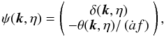 (A.1)where θ
is the divergence of the velocity field,
θ = ∇·v,
η = lnD(z)
where D(z) is the linear growth factor (normalized by
D(0) = 1 today),
ȧ = da/dt
where a(t) is the scale factor, and
f = dlnD/dlna. Then, introducing
the coordinate
x = (k,η,i), where
i = 1 or 2 is the discrete index of the two-component vectors, the
equations of motion write as (Valageas 2007a)
(A.1)where θ
is the divergence of the velocity field,
θ = ∇·v,
η = lnD(z)
where D(z) is the linear growth factor (normalized by
D(0) = 1 today),
ȧ = da/dt
where a(t) is the scale factor, and
f = dlnD/dlna. Then, introducing
the coordinate
x = (k,η,i), where
i = 1 or 2 is the discrete index of the two-component vectors, the
equations of motion write as (Valageas 2007a)
 (A.2)where the matrix
 reads as
  (A.3)whereas
the symmetric vertex
Ks(x;x1,x2) = Ks(x;x2,x1)
writes as
(A.3)whereas
the symmetric vertex
Ks(x;x1,x2) = Ks(x;x2,x1)
writes as  (A.4)with
 and
zero otherwise (Crocce & Scoccimarro
2006b). In addition to the usual two-point correlation function,
and
zero otherwise (Crocce & Scoccimarro
2006b). In addition to the usual two-point correlation function,  (A.8)resummation schemes often
involve the response function (or propagator), defined as the functional derivative of the
nonlinear field ψ with respect to an infinitesimal “noise”
ζ that would be added to the right hand side of the equation of
motion (A.2),
(A.8)resummation schemes often
involve the response function (or propagator), defined as the functional derivative of the
nonlinear field ψ with respect to an infinitesimal “noise”
ζ that would be added to the right hand side of the equation of
motion (A.2),  (A.9)As described in
Valageas (2007a, 2008), the nonlinear correlation and response functions obey the exact
Schwinger-Dyson equations
(A.9)As described in
Valageas (2007a, 2008), the nonlinear correlation and response functions obey the exact
Schwinger-Dyson equations  where
Σ(x,y) and Π(x,y) are “self-energy” terms, that can be
written as diagrammatic expansions over the linear two-point
functions CL and RL.
Equation (A.10) can be integrated as
where
Σ(x,y) and Π(x,y) are “self-energy” terms, that can be
written as diagrammatic expansions over the linear two-point
functions CL and RL.
Equation (A.10) can be integrated as
 (A.12)where
CL(ηI) is the linear correlation
function at an early time ηI, with
ηI → − ∞, and the first product
“ × CL × ” does not contain any integration over time.
(A.12)where
CL(ηI) is the linear correlation
function at an early time ηI, with
ηI → − ∞, and the first product
“ × CL × ” does not contain any integration over time.
Then, at 1-loop order the direct steepest-descent scheme amounts to use for Σ and Π their lowest order terms, over powers of CL and RL. This means that Eq. (A.12) for the correlation C reads as the first line in Fig. 1, while a similar diagrammatic expression holds for the response R (see Fig. 8 in Valageas 2008). In particular, solving Eq. (A.11) as a perturbative series over powers of Σ gives a diagrammatic expansion for the response R in terms of “bubble” diagrams, and substituting into Eq. (A.12) this gives the series of diagrams shown in the second equality of Fig. 1. In practice, one does not compute the two-point function C(x,y), whence the density power spectrum, from these diagrammatic series, but from the integro-differential Eq. (A.11) and the explicit expression (A.12).
First, using in the following the approximation
Ωm/f2 ≃ 1, the linear correlation and response
functions read as  (A.13)where
PL0(k) is the linear density power spectrum
today (when η = 0), and
(A.13)where
PL0(k) is the linear density power spectrum
today (when η = 0), and ![Mathematical equation: \appendix \setcounter{section}{1} \begin{eqnarray} R_{\rm L}\left(x_1,x_2\right) & = & \theta\left(\eta_1-\eta_2\right) \, \delta_{\rm D}\left(\vk_1-\vk_2\right) \nonumber \\ \label{R0R0pR0m} && \times \left[{\rm e}^{\eta_1-\eta_2} R_0^+ + {\rm e}^{-3\left(\eta_1-\eta_2\right)/2} R_0^- \right], \end{eqnarray}](/articles/aa/full_html/2011/03/aa15685-10/aa15685-10-eq424.png) (A.14)with
(A.14)with
 (A.15)In Eq. (A.14) the Heaviside factor
θ(η1 − η2)
expresses the causality of the response function. Then, the “self-energy” terms read at
lowest order as (Valageas 2007a)
(A.15)In Eq. (A.14) the Heaviside factor
θ(η1 − η2)
expresses the causality of the response function. Then, the “self-energy” terms read at
lowest order as (Valageas 2007a) ![Mathematical equation: \appendix \setcounter{section}{1} \begin{eqnarray} \Sigma_0\left(x_1,x_2\right) & = & \theta\left(\eta_1-\eta_2\right) \, \delta_{\rm D}\left(\vk_1-\vk_2\right) \nonumber \\ \label{S0S0pS0m} && \times \left[{\rm e}^{2\eta_1} \Sigma_0^+\left(k_1\right) + {\rm e}^{-\eta_1/2+5\eta_2/2} \Sigma_0^-\left(k_1\right) \right], \end{eqnarray}](/articles/aa/full_html/2011/03/aa15685-10/aa15685-10-eq427.png) (A.16)with
(A.16)with
 (A.17)and
 (A.18)with
  (A.19)These
“self-energy” terms also satisfy the symmetries
(A.19)These
“self-energy” terms also satisfy the symmetries  (A.20)Thanks to the
simple time dependence of
Σ0(x1,x2), which
arises from the fact that we have expanded Σ over the linear two-point
functions CL and RL and only
kept the lowest order term, it is possible to eliminate the integral terms in the
Schwinger-Dyson Eq. (A.11) by taking
successive derivatives with respect to η1. This yields
(A.20)Thanks to the
simple time dependence of
Σ0(x1,x2), which
arises from the fact that we have expanded Σ over the linear two-point
functions CL and RL and only
kept the lowest order term, it is possible to eliminate the integral terms in the
Schwinger-Dyson Eq. (A.11) by taking
successive derivatives with respect to η1. This yields
![Mathematical equation: \appendix \setcounter{section}{1} \begin{eqnarray} \lefteqn{\frac{\pl^3 R_1}{\pl\eta_1^3} - \frac{3}{2} \frac{\pl^2 R_1}{\pl\eta_1^2} -\frac{\pl^2 R_2}{\pl\eta_1^2} - \frac{\pl R_1}{\pl\eta_1} + \frac{3}{2} \frac{\pl R_2}{\pl\eta_1} + R_2 = } \nonumber \\[1.5mm] \label{R01diff} &&{\rm e}^{2\eta_1} \left[\left(\Sigma_{0;11}^+ + \Sigma_{0;22}^+\right) \frac{\pl R_1}{\pl\eta_1} + \frac{5}{2} \Sigma_{0;11}^+ R_1 + \frac{5}{2} \Sigma_{0;12}^+ R_2 \right] \end{eqnarray}](/articles/aa/full_html/2011/03/aa15685-10/aa15685-10-eq434.png) (A.21)
(A.21)![Mathematical equation: \appendix \setcounter{section}{1} \begin{eqnarray} \lefteqn{\frac{\pl^3 R_2}{\pl\eta_1^3} - \frac{3}{2} \frac{\pl^2 R_1}{\pl\eta_1^2} -\frac{\pl^2 R_2}{\pl\eta_1^2} + \frac{9}{4} \frac{\pl R_1}{\pl\eta_1} - \frac{7}{4} \frac{\pl R_2}{\pl\eta_1} + \frac{3}{2} R_1 - \frac{1}{2} R_2 = } \nonumber \\[1.5mm] \label{R02diff} &&{\rm e}^{2\eta_1} \left[ \left(\Sigma_{0;11}^+ + \Sigma_{0;22}^+\right) \frac{\pl R_2}{\pl\eta_1} + \frac{5}{2} \Sigma_{0;21}^+ R_1 + \frac{5}{2} \Sigma_{0;22}^+ R_2 \right] \end{eqnarray}](/articles/aa/full_html/2011/03/aa15685-10/aa15685-10-eq435.png) (A.22)where
the pair (R1,R2) corresponds
either to (R11,R21) or
(R12,R22). These equations apply
to η1 > η2 and the initial
conditions at η1 = η2 are
(A.22)where
the pair (R1,R2) corresponds
either to (R11,R21) or
(R12,R22). These equations apply
to η1 > η2 and the initial
conditions at η1 = η2 are
![Mathematical equation: \appendix \setcounter{section}{1} \begin{eqnarray} \label{Xdef} X^T & = & \left(\bea{cccccc} R_1 & R_2 & \frac{\pl R_1}{\pl\eta_1} & \frac{\pl R_2}{\pl\eta_1} & \frac{\pl^2 R_1}{\pl\eta_1^2} & \frac{\pl^2 R_2}{\pl\eta_1^2} \ea \right) \\[1.5mm] \label{X1} & = & \left(\bea{cccccc} 1 & 0 & 0 & \frac{3}{2} & \frac{3}{2}+{\rm e}^{2\eta_1}\left(\Sigma_{0;11}^+ + \Sigma_{0;22}^+\right) & - \frac{3}{4} \ea \right) \end{eqnarray}](/articles/aa/full_html/2011/03/aa15685-10/aa15685-10-eq441.png) for
the pair (R11,R21), and
for
the pair (R11,R21), and
 (A.25)for
the pair (R12,R22). Thus, we
obtain the response function by solving the differential Eqs. (A.21), (A.22), with the initial conditions (A.24), (A.25), using
an ordinary Runge-Kutta algorithm. A great simplification is that there are no longer
integral terms over past times in the right hand side of Eqs. (A.21), (A.22), so that numerical computations are very fast.
(A.25)for
the pair (R12,R22). Thus, we
obtain the response function by solving the differential Eqs. (A.21), (A.22), with the initial conditions (A.24), (A.25), using
an ordinary Runge-Kutta algorithm. A great simplification is that there are no longer
integral terms over past times in the right hand side of Eqs. (A.21), (A.22), so that numerical computations are very fast.
Finally, it is possible to take advantage of the factorized time dependence
of Π0 in Eq. (A.18) to
factorize Eq. (A.12). To compute the first
product in Eq. (A.12) we define the
two-component vector  (A.26)while for the second
product we diagonalize the symmetric matrix Π0 as
(A.26)while for the second
product we diagonalize the symmetric matrix Π0 as  (A.27)where p ±
are the eigenvalues of Π0 and π ± its normalized
eigenvectors, and we define the two-component vectors,
(A.27)where p ±
are the eigenvalues of Π0 and π ± its normalized
eigenvectors, and we define the two-component vectors,  (A.28)Then, Eq. (A.12) writes as
 ![Mathematical equation: \appendix \setcounter{section}{1} \begin{eqnarray} C\left(k;\eta_1,\eta_2\right) & = & \varphi^{\rm I}\left(\eta_1\right) \cdot \varphi^{\rm I}\left(\eta_2\right)^T \nonumber \\[1.5mm] \label{C-fact} && \hspace{-1.5cm} + p^+ \, \varphi^+\left(\eta_1\right) \cdot \varphi^+\left(\eta_2\right)^T + p^- \, \varphi^-\left(\eta_1\right) \cdot \varphi^-\left(\eta_2\right)^T. \end{eqnarray}](/articles/aa/full_html/2011/03/aa15685-10/aa15685-10-eq449.png) (A.29)In
particular, the nonlinear power spectrum is given by the equal-time upper-left component
of the correlation matrix C,
(A.29)In
particular, the nonlinear power spectrum is given by the equal-time upper-left component
of the correlation matrix C,  (A.30)The factorized
form (A.29), which avoids to compute
two-dimensional integrals over past times as in generic expressions of Eq. (A.12), thanks to the factorized time
dependence of Π0 in Eq. (A.18),
again allows fast numerical computations.
(A.30)The factorized
form (A.29), which avoids to compute
two-dimensional integrals over past times as in generic expressions of Eq. (A.12), thanks to the factorized time
dependence of Π0 in Eq. (A.18),
again allows fast numerical computations.
All Tables
All Figures
|
Fig. 1 The resummation performed by the “direct steepest-descent” method at one-loop order, for the two-point correlation C. The blue single lines are the linear correlation CL and the red single lines are the linear response (propagator) RL. The double red lines in the first equality are the nonlinear response R (at that order), which contains an infinite series of bubble diagrams, and explicit substitution gives the series of diagrams shown in the second equality below. |
| In the text | |
|
Fig. 2 Wavenumber ranges covered by our N-body simulations, from the fundamental mode (left edge) to the mean inter-particle scale (solid right edge) and to the softening scale (dashed right edge). Left: the four main simulations, middle: simulations used in Test 1, right: simulations used in Test 2. |
| In the text | |
|
Fig. 3 The ratio of the power spectrum to the highest resolution run, L9-N11. The three lines correspond to L9-N10, L9-N9 and L9-N8 from top to bottom. Left: z = 3, middle: z = 1, right: z = 0.35. |
| In the text | |
 |
Fig. 4 Same as Fig. 3, but for two-point correlation function. |
| In the text | |
|
Fig. 5 The ratio of the power spectrum to the largest volume run, L12-N11. The three symbols correspond to L11-N10 (triangles), L10-N9 (circles) and L9-N8 (diamonds). Left: z = 3, middle: z = 1, right: z = 0.35. |
| In the text | |
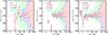 |
Fig. 6 Same as Fig. 5, but for the two-point correlation function. |
| In the text | |
|
Fig. 7 1-σ statistical error of the power spectrum (fractional) estimated from Eq. (45) for L9-N11, L10-N11, L11-N11 and L12-N11 (from top to bottom). |
| In the text | |
|
Fig. 8 The probability F2H(1/k) that a Lagrangian pair of distance q = 1/k belongs to different halos, from Eq. (21). We show our results for z = 0.35, 1, and 3. |
| In the text | |
|
Fig. 9 The power per logarithmic interval of k, as defined in Eq. (47), at redshifts
z = 0.35, 1, and 3. The symbols are the results from the numerical
simulations described in Sect. 4. The black
solid line is the linear power spectrum, |
| In the text | |
|
Fig. 10 The ratio of the nonlinear power spectrum P(k) to a smooth linear power spectrum PLs without acoustic baryonic oscillations, from Eisenstein & Hu (1999). The points with error bars are the results from N-body simulations. The black solid line PL is the linear power spectrum, and the upper blue dashed line P1loop is the prediction of standard perturbation theory up to one-loop order. The green solid line P is the full nonlinear power spectrum, from Eq. (22), whereas the lower blue dotted line Ppert is the perturbative part. The magenta dot-dashed line PS is the fit to simulations from Smith et al. (2003) (which was not specifically designed to reproduce the baryon oscillations). |
| In the text | |
|
Fig. 11 The power per logarithmic interval of k, as in Fig. 9, but for halos that are defined either by a density contrast δ = 200 (solid curves, identical to those of Fig. 9), or by δ = 50 (dot-dashed curves). Both the 1-halo contribution Δ1H and the full nonlinear power spectrum Δ2 are shown. |
| In the text | |
|
Fig. 12 The ratio of the nonlinear power spectrum P(k) to a smooth linear power spectrum PLs without acoustic baryonic oscillations, as in Fig. 12, for halos defined by δ = 200 (green solid curves, identical to those of Fig. 10), or by δ = 50 (red dot-dashed curves). |
| In the text | |
|
Fig. 13 The ratio of the nonlinear power spectrum P(k) to
a “no-wiggle” linear power
spectrum PLs(k), as
in Fig. 10, at redshifts
z = 0.35, 1, and 3. The green solid lines correspond to our
fiducial model, with halos defined by a density contrast δ = 200,
and are identical to the green solid lines shown in Fig. 10, while the red dashed lines are obtained by setting to zero
the 1-halo counterterm |
| In the text | |
|
Fig. 14 The ratio of the nonlinear power spectrum P(k) to a “no-wiggle” linear power spectrum PLs(k), as in Fig. 10, at redshifts z = 0.35, 1, and 3. The green solid lines “resum” correspond to our model as in Fig. 10, whereas the blue dashed lines correspond to the approximation P2H = PL (it cannot be distinguished from the linear power PL on these scales at z = 3). |
| In the text | |
|
Fig. 15 The power per logarithmic interval of k, as in Fig. 9, at redshifts z = 0.35, 1, and 3. We plot the curves obtained with our model (green solid lines) and with the approximation P2H = PL (blue dashed lines), as in Fig. 14. |
| In the text | |
|
Fig. 16 The ratio of the nonlinear power spectrum P(k) to a “no-wiggle” linear power spectrum PLs(k), as in Fig. 10, at redshifts z = 0.35, 1, and 3. The red dashed lines “SPT” correspond to the use of 1-loop “Standard Perturbation Theory” for the term Ppert in the 2-halo contribution (27), whereas the blue solid lines “DR” correspond to the use of the “Decaying Response” function from Crocce & Scoccimarro (2006a) in the external double lines of the two upper diagrams of Fig. 1. The 1-halo term is the same as the one used in Sect. 5. |
| In the text | |
|
Fig. 17 The power per logarithmic interval of k, as in Fig. 9, at redshifts z = 0.35, 1, and 3. We plot the curves obtained using 1-loop “standard perturbation theory” (red dashed lines for the full nonlinear power Δ2, and lower red dotted lines for the associated 2-halo contribution) or the “decaying response” function from Crocce & Scoccimarro (2006a) (blue solid lines for the full nonlinear power Δ2, and lower blue dotted lines for the associated 2-halo contribution). Both the full and 2-halo power spectra obtained with “SPT” are larger than their “DR” counterparts. |
| In the text | |
|
Fig. 18 The ratio of the nonlinear power spectrum P(k) to a “no-wiggle” linear power spectrum PLs(k), as in Fig. 10, at redshifts z = 0.35, 1, and 3. The red dot-dashed lines “PMat” correspond to the use of the Lagrangian-based 1-loop expansion (53) for the term Ppert in the 2-halo contribution (27), whereas the blue solid lines “PmZ” correspond to the use of the “modified Zeldovich” expansion (56). The 1-halo term is the same as the one used in Sect. 5. |
| In the text | |
|
Fig. 19 The real-space two-point correlation function ξ(x), at redshifts z = 0.35, 1, and 3. The symbols are the results from the numerical simulations described in Sect. 4. The black dashed line is the linear correlation, ξL, and the blue dotted line which is somewhat below at low x is the 2-halo contribution ξ2H. The steep solid line xi1H is the 1-halo contribution, for the halo model described in Sect. 3.2. The green solid line is the full nonlinear correlation function, ξ = ξ2H + ξ1H. |
| In the text | |
|
Fig. 20 The real-space two-point correlation function ξ(x), at redshifts z = 0.35, 1, and 3, as in Fig. 19 but on larger scales. Since the 1-halo contribution is negligible on these scales we only show the linear correlation (black dashed line) and the full nonlinear correlation (green solid line). |
| In the text | |
|
Fig. 21 The two-point correlation ξ(x), as in Fig. 19, but for halos that are defined either by a density contrast δ = 200 (solid curves, identical to those of Fig. 19), or by δ = 50 (dot-dashed curves). |
| In the text | |
|
Fig. 22 The accuracy of our model and our simulations at redshifts z = 0.35, 1, and 3, for the density power spectrum. The green solid line is the relative difference between the model and the simulations, from Eq. (60). The dashed line that grows at low k is the relative statistical error (45) of the simulations, while the dashed line that grows at high k is the relative shot-noise error. |
| In the text | |
|
Fig. 23 The accuracy of our model and our simulations at redshifts z = 0.35, 1, and 3, for the density two-point correlation. The green solid line is the relative difference between the model and the simulations, from Eq. (61). The dashed line that grows at large x is the relative statistical error (46) of the simulations, while the dashed line that grows at small x is the relative shot-noise error. |
| In the text | |
Current usage metrics show cumulative count of Article Views (full-text article views including HTML views, PDF and ePub downloads, according to the available data) and Abstracts Views on Vision4Press platform.
Data correspond to usage on the plateform after 2015. The current usage metrics is available 48-96 hours after online publication and is updated daily on week days.
Initial download of the metrics may take a while.