| Issue |
A&A
Volume 527, March 2011
|
|
|---|---|---|
| Article Number | A138 | |
| Number of page(s) | 20 | |
| Section | Astrophysical processes | |
| DOI | https://doi.org/10.1051/0004-6361/201015568 | |
| Published online | 11 February 2011 | |
The baroclinic instability in the context of layered accretion
Self-sustained vortices and their magnetic stability in local compressible unstratified models of protoplanetary disks
1
Max-Planck-Institut für Astronomie, Königstuhl 17, 69117
Heidelberg,
Germany
2
American Museum of Natural History, Department of
Astrophysics, Central Park West at
79th Street, New
York, NY
10024-5192,
USA
e-mail: This email address is being protected from spambots. You need JavaScript enabled to view it.
Received:
11
August
2010
Accepted:
29
November
2010
Abstract
Context. Turbulence and angular momentum transport in accretion disks remains a topic of debate. With the realization that dead zones are robust features of protoplanetary disks, the search for hydrodynamical sources of turbulence continues. A possible source is the baroclinic instability (BI), which has been shown to exist in unmagnetized non-barotropic disks.
Aims. We aim to verify the existence of the baroclinic instability in 3D magnetized disks, as well as its interplay with other instabilities, namely the magneto-rotational instability (MRI) and the magneto-elliptical instability.
Methods. We performed local simulations of non-isothermal accretion disks with the Pencil Code. The entropy gradient that generates the baroclinic instability is linearized and included in the momentum and energy equations in the shearing box approximation. The model is compressible, so excitation of spiral density waves is allowed and angular momentum transport can be measured.
Results. We find that the vortices generated and sustained by the baroclinic instability in the purely hydrodynamical regime do not survive when magnetic fields are included. The MRI by far supersedes the BI in growth rate and strength at saturation. The resulting turbulence is virtually identical to an MRI-only scenario. We measured the intrinsic vorticity profile of the vortex, finding little radial variation in the vortex core. Nevertheless, the core is disrupted by an MHD instability, which we identify with the magneto-elliptic instability. This instability has nearly the same range of unstable wavelengths as the MRI, but has higher growth rates. In fact, we identify the MRI as a limiting case of the magneto-elliptic instability, when the vortex aspect ratio tends to infinity (pure shear flow). We isolated its effect on the vortex, finding that a strong but unstable vertical magnetic field leads to channel flows inside the vortex, which stretch it apart. When the field is decreased or resistivity is used, we find that the vortex survives until the MRI develops in the box. The vortex is then destroyed by the strain of the surrounding turbulence. Constant azimuthal fields and zero net flux fields also lead to vortex destruction. Resistivity quenches both instabilities when the magnetic Reynolds number of the longest vertical wavelength of the box is near unity.
Conclusions. We conclude that vortex excitation and self-sustenance by the baroclinic instability in protoplanetary disks is viable only in low ionization, i.e., the dead zone. Our results are thus in accordance with the layered accretion paradigm. A baroclinicly unstable dead zone should be characterized by the presence of large-scale vortices whose cores are elliptically unstable, yet sustained by the baroclinic feedback. Since magnetic fields destroy the vortices and the MRI outweighs the BI, the active layers are unmodified.
Key words: accretion, accretion disks / hydrodynamics / instabilities / magnetohydrodynamics (MHD) / turbulence / methods: numerical
© ESO, 2011
1. Introduction
Turbulence is the preferred mechanism for enabling accretion in circumstellar disks, and the magneto-rotational instability (MRI, Balbus & Hawley 1991) is the preferred route to turbulence. However, the MRI requires sufficient ionization since the magnetic field and the gas must be coupled, so it should not be expected to occur in regions of low ionization such as the “dead zone” (Gammie 1996; Turner & Drake 2009). Therefore, the search for hydrodynamical sources of turbulence continues, if only to provide some residual accretion in the dead zone. A distinct possibility is the baroclinic instability (BI; Klahr & Bodenheimer 2003; Klahr 2004), the interest in which has been recently rekindled (Petersen et al. 2007a,b; Lesur & Papaloizou 2010).
A baroclinic flow is one where the pressure depends on both density and temperature, as opposed to a barotropic flow where the pressure only depends on density. In such a flow, the non-axyssimmetric misalignment between surfaces of constant density ρ (isopycnals) and surfaces of constant pressure p (isobars) generates vorticity. Mathematically, this translates into a non-zero baroclinic vector, ∇ × (−ρ-1∇p) = ρ-2∇p × ∇ρ. Baroclinicity has long been known in atmospheric dynamics to be responsible for turbulent patterns on planets and for weather patterns of Rossby waves (planetary waves), cyclones, and anticyclones on Earth.
The difference between the baroclinic instability of weather patterns on planetary atmospheres and the baroclinic instability in accretion disks is that the former is linear, whereas the latter is nonlinear (Klahr 2004; Lesur & Papaloizou 2010). This is because in accretion disks, the disturbances have to overcome the strong Keplerian shear that causes perturbations to be heavily dominated by restoring forces in all Reynolds numbers.
Simulation suite parameters for nonmagnetic runs and results.
The nature of the instability was clarified in the work of Petersen et al. (2007a,b), who highlighted the importance of finite thermal inertia. When the thermal time is comparable to the eddy turnover time, the vortex is able to establish an entropy gradient around itself that compensates the large-scale entropy gradient that created it. This entropy gradient back reacts on the eddy, generating more vorticity via buoyancy. This in turn reinforces the gradient. A positive feedback has been established, and the eddy grows. This, in a nutshell, is the baroclinic instability: the sole result of an eddy trying to counter the background entropy gradient that established it, and reinforcing itself by doing so.
The 3D properties of the instability have been studied by Lesur & Papaloizou (2010). They find that the vortices produced are not destroyed when baroclinicity is present, although they are unstable to the elliptical instability (Kerswell 2002; Lesur & Papaloizou 2009). The saturated state of the instability is dominated by the presence of large-scale 3D, self-sustained, vortices with weakly turbulent cores. The study of Petersen et al. (2007a,b) and most of that of Lesur & Papaloizou (2010) was done with spectral codes, which filter sound waves. Vortices, however, have the interesting property of radiating inertial-acoustic waves, which are known to transport angular momentum (Heinemann & Papaloizou 2009). Lesur & Papaloizou (2010) performed a compressible, yet 2D, simulation, with a resulting Shakura-Sunyaev-like α value of 10-3.
These results are intriguing, and a major question to ask is what their significance is in the context of the layered accretion paradigm. Vortices have been described in the literature as devoid of radial shear (Klahr & Bodenheimer 2006), so in principle they could form and survive in the midst of MRI turbulence, as the simulations of Fromang & Nelson (2005) suggest. Moreover, if the baroclinic instability is able to produce and sustain vortices when magnetization is present, synergy with the MRI is an interesting possibility, potentially leading to higher accretion rates than hitherto achieved in previous works. On the other hand, elliptical streamlines can be heavily destabilized by magnetic fields (Lebovitz & Zweibel 2004; Mizerski & Bajer 2009). This magneto-elliptic instability may either be stabilized by baroclinicity, as the elliptic instability was shown to be (Lesur & Papaloizou 2010), or completely break the vortices apart thus rendering the baroclinic instability meaningless in the presence of magnetization. We address these open questions in this work.
The paper is structured as follows. In Sect. 2 we introduce the model equations of the compressible shearing box, modified to include the contribution from the large-scale background entropy gradient. In view of the controversy aroused by the baroclinic instability in the literature, it was found prudent to establish the reliability of the numerics, as well as to provide an independent confirmation of the 2D results. This is done in Sect. 3. The 3D results are presented in Sect. 4. Tables 1 and 2 contain summaries of the simulations performed for this study, referring to the sections and figures they are described. Conclusions are given in Sect. 5.
Simulation suite parameters for magnetic runs.
2. The model
We model a local patch of the disk following the shearing box approximation. The reader is
referred to Regev & Umurhan (2008) for an
extensive discussion of the limitations of the approximation. To include the baroclinic
term, we consider a large-scale radial pressure gradient following a power law of
index ξ where r is the cylindrical
radius and R0 is a reference radius. The overbar indicates that
this quantity is time-independent. The total pressure is
where r is the cylindrical
radius and R0 is a reference radius. The overbar indicates that
this quantity is time-independent. The total pressure is
 ,
where p is the local fluctuation. The linearization of this gradient is
done in the same way as the large-scale Keplerian shear is linearized in the shearing box.
This leads to extra terms in the equations involving the radial pressure gradient. We quote
the modified shearing box equations below. A derivation of the extra terms is presented in
Appendix A.
,
where p is the local fluctuation. The linearization of this gradient is
done in the same way as the large-scale Keplerian shear is linearized in the shearing box.
This leads to extra terms in the equations involving the radial pressure gradient. We quote
the modified shearing box equations below. A derivation of the extra terms is presented in
Appendix A.  In the equations above,
u is the velocity, A the
magnetic vector potential,
B = ∇ × A the
magnetic field,
J = ∇ × B/μ0
the current (where μ0 is the magnetic permittivity),
η is the resistivity, T the temperature,
s the entropy, and K the radiative conductivity. The
operator
In the equations above,
u is the velocity, A the
magnetic vector potential,
B = ∇ × A the
magnetic field,
J = ∇ × B/μ0
the current (where μ0 is the magnetic permittivity),
η is the resistivity, T the temperature,
s the entropy, and K the radiative conductivity. The
operator  (5)represents the Keplerian derivative of a fluid
parcel. It is the only place where the Keplerian flow
(5)represents the Keplerian derivative of a fluid
parcel. It is the only place where the Keplerian flow
 appears explicitly. The advection is made
Galilean-invariant by means of the SAFI algorithm (Johansen et al. 2009), which speeds up performance. The simulations were done with the
Pencil Code1.
appears explicitly. The advection is made
Galilean-invariant by means of the SAFI algorithm (Johansen et al. 2009), which speeds up performance. The simulations were done with the
Pencil Code1.
We work with entropy as the main thermodynamical quantity. This is a natural choice when
dealing with baroclinicity. Considering the polytropic equation of state,
 (6)and the definition of entropy,
 ![Mathematical equation: \begin{equation} s=\cv\left[\ln(p/p_0)-\gamma\ln(\rho/\rho_0)\right], \label{eq:entropy} \end{equation}](/articles/aa/full_html/2011/03/aa15568-10/aa15568-10-eq67.png) (7)we immediately recognize
s = cVln(k/k0)
in the case n = 1/(γ − 1); i.e., up to a constant, entropy
is the proportionality factor in the polytropic equation of state. That means that any
spatial gradient of entropy translates into a departure from barotropic conditions2.
(7)we immediately recognize
s = cVln(k/k0)
in the case n = 1/(γ − 1); i.e., up to a constant, entropy
is the proportionality factor in the polytropic equation of state. That means that any
spatial gradient of entropy translates into a departure from barotropic conditions2.
The third term on the right-hand side of the entropy equation is an artificial thermal
relaxation term, which drives the temperature back to the initial temperature
T0, on a pre-specified thermal
timescale τc. The temperature is
![Mathematical equation: \hbox{$T = c_{\rm s}^2/\left[c_{\rm p}(\gamma-1)\right]$}](/articles/aa/full_html/2011/03/aa15568-10/aa15568-10-eq71.png) , where cs is the
sound speed,
γ = cp/cV
the adiabatic index, and
, where cs is the
sound speed,
γ = cp/cV
the adiabatic index, and  and cp are the
heat capacities at constant volume and constant pressure, respectively.
and cp are the
heat capacities at constant volume and constant pressure, respectively.
 |
Fig. 1 Snapshots of the fiducial 2D run with ξ = 2, τ = 2π, H = 0.1, and resolution 2562. A vortex is formed and establishes a local entropy gradient that counteracts the global entropy gradient that caused it in first place. Moderate cooling times keep the surfaces of constant density and constant pressure misaligned, leading to more vortex growth. In the positive feedback that ensues, giant anti-cyclonic vortices grow to the sonic scale. The initial condition was free of enstrophy. This vorticity growth was due purely to baroclinic effects. |
After defining entropy, we also define the Brunt-Väisälä frequency N, the
frequency associated with buoyant structures  (8)and we have assumed axis-symmetry
(∂φ = 0) and no vertical stratification
(∂z = 0) between the steps. In our setup,
there is no large-scale density gradient, so the first term inside the parentheses cancel.
As dp/dr = − pξ/r, we
have, at
r = R0
(8)and we have assumed axis-symmetry
(∂φ = 0) and no vertical stratification
(∂z = 0) between the steps. In our setup,
there is no large-scale density gradient, so the first term inside the parentheses cancel.
As dp/dr = − pξ/r, we
have, at
r = R0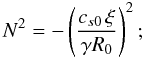 (9)i.e., the Brunt-Väisälä frequency is always
imaginary. However, the flow is convectively stable, since the epicyclic frequency squared
(9)i.e., the Brunt-Väisälä frequency is always
imaginary. However, the flow is convectively stable, since the epicyclic frequency squared
 (10)is far higher than
− N2, so that the Solberg-Høiland criterion is always
satisfied
(10)is far higher than
− N2, so that the Solberg-Høiland criterion is always
satisfied  (11)In Eq. (10), j = Ωr2 is the
specific angular momentum per unit mass.
(11)In Eq. (10), j = Ωr2 is the
specific angular momentum per unit mass.
We add explicit sixth-order hyperdiffusion fD(ρ), hyperviscosity fν(u,ρ), and hyperresistivity fη(A) to the mass, momentum, and induction equations as specified in Lyra et al. (2008). Hyper heat conductivity fK(s) to the entropy equation is added as in Lyra et al. (2009) and Oishi & Mac Low (2009). All simulations use cp = R0 = Ω0 = ρ0 = μ0 = 1, γ = 1.4, and cs = 0.1.
3. 2D results
Although the most interesting results for the effects of the baroclinic generation of
vorticity should be given by 3D models, the existence of the baroclinic instability has been
strongly contested even in two dimensions. We therefore consider it important to present 2D
results confirming its excitation. In Fig. 1 we present
a fiducial 2D run where the evolution of the baroclinic instability is followed. It
corresponds to run A in Table 1. The slope of the
entropy gradient is ξ = 2, which corresponds to a Richardson number
 . As initial condition, we seed the box with
noise at small wavenumbers only, following
. As initial condition, we seed the box with
noise at small wavenumbers only, following  (12)The phase 0 < φ < 1
determines the randomness. The subscripts underscore that the phase is the same for all grid
points, only changing with wavenumber. The constant C sets the strength of
the perturbation. As stressed by Lesur & Papaloizou (2010), the baroclinic instability is subcritical, and therefore a finite initial
amplitude is needed to trigger growth. We set the constant C to yield
Σrms = 0.05. The entropy is then initialized such that
p = p0 ≡ const. in the
sheet.
(12)The phase 0 < φ < 1
determines the randomness. The subscripts underscore that the phase is the same for all grid
points, only changing with wavenumber. The constant C sets the strength of
the perturbation. As stressed by Lesur & Papaloizou (2010), the baroclinic instability is subcritical, and therefore a finite initial
amplitude is needed to trigger growth. We set the constant C to yield
Σrms = 0.05. The entropy is then initialized such that
p = p0 ≡ const. in the
sheet.
The rationale behind this unorthodox initial condition is that this noise is independent of resolution. The usual Gaussian noise distributes power through all wavelengths, so the wavelengths from k < 10 are assigned increasingly less power as the resolution increases. We stress that it is not vital for the instability to be seeded with resolution-independent noise, nor are we missing important physics by not exciting the small scales.
We do not seed noise in the velocity field. The initial condition is strictly nonvortical. Since in 2D the stretching term is absent, any increase in vorticity can only be a baroclinic effect.
3.1. Baroclinic production of vorticity
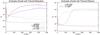 |
Fig. 2 Left. Baroclinic enstrophy growth with thermal relaxation, where a gas parcel returns to the initial temperature on a timescale τ. A stable entropy gradient can only be maintained between the extremes of too fast a relaxation (isothermal behavior) and too slow a relaxation (adiabatic behavior). Optimal growth occurs when τ is comparable to the dynamical time. Right. Baroclinic enstrophy growth with thermal diffusion, where heat diffuses over a scale height on a timescale τ. Optimal growth occurs on longer timescales when compared to the thermal relaxation case. |
The baroclinic term, in 2D, is  (13)The two first terms are local, whereas the
third comes from the large-scale gradient. There would be a fourth if we considered a
large-scale density gradient as well. This third term generates vorticity out of any
azimuthal perturbation in the density, much in the same way as the locally isothermal
approximation does in global disks. This term is paramount, since it is the only source
term that will generate net enstrophy in the flow. In the beginning, this term dominates,
generating enstrophy out of the initial density perturbations. The enstrophy is then
amplified by the local baroclinic vector via the positive feedback described in the
introduction.
(13)The two first terms are local, whereas the
third comes from the large-scale gradient. There would be a fourth if we considered a
large-scale density gradient as well. This third term generates vorticity out of any
azimuthal perturbation in the density, much in the same way as the locally isothermal
approximation does in global disks. This term is paramount, since it is the only source
term that will generate net enstrophy in the flow. In the beginning, this term dominates,
generating enstrophy out of the initial density perturbations. The enstrophy is then
amplified by the local baroclinic vector via the positive feedback described in the
introduction.
We witness the same general phenomena as Petersen et al. (2007a), even though the details of implementating the entropy gradient are different. In global simulations, the vortex swings gas parcels back and forth from cold to hot, which causes baroclinicity and vortex growth. Here the initial temperature all over the box is the same, so the vortex does not automatically swing gas from cold to hot. It swings it up and down the hard-coded pressure (= temperature = entropy) gradient. The second-to-last term on the right-hand side of the entropy equation comes from the linearization of the advection term in the presence of an entropy gradient. It embodies how the relative entropy of a fluid parcel with respect to the background entropy changes as it walks up or down an entropy gradient, clearly demonstrated by the dependence on ux. Because the movement along the vortex lines is embedded with a ux component of motion, this term increases or decreases the entropy within the gas parcel depending on the sign of ux. Of course, this is just the same physical effect in a different frame of reference.
We show a time series of the flow in Fig. 1 as snapshots of density, pressure, entropy, and vorticity. From these snapshots we see that the density and the pressure are very correlated. One would therefore expect that the amount of baroclinicity produced is tiny or vanishingly small. However, looking at the snapshots of entropy, we see that appearances are deceiving: the vortex generates a strong radial entropy gradient around itself. This is what we described qualitatively in the introduction, and what Petersen et al. (2007a,b) called a “sandwich pattern”. Notice that the sign is indeed reversed with respect to the global gradient (higher at negative values of x). This pattern of a local entropy gradient developed by the vortex is a constant feature throughout the simulations.
 |
Fig. 3 Enstrophy and the resulting alpha-viscosity for the fiducial 2D run. The two quantities are quite well correlated, since the angular momentum transport is the result of inertial-acoustic waves, which in turn are driven by vorticity. |
3.2. Angular momentum transport
A very important question to ask is what is the strength of the angular momentum
transport of the resulting baroclinic unstable flow. We measured the kinetic alpha values
in the simulations,  (14)where
  is the Reynolds stress. The value measured
is α ≈ 5 × 10⁻³, indicating good transport of angular
momentum. The temporal variation of alpha (Fig. 3)
matches that of the enstrophy.
is the Reynolds stress. The value measured
is α ≈ 5 × 10⁻³, indicating good transport of angular
momentum. The temporal variation of alpha (Fig. 3)
matches that of the enstrophy.
This correlation is understood in light of the shear-vortex wave coupling. The angular momentum transport does not come from the vortex itself, but is instead caused by the inertial-acoustic waves that are driven by vorticity. For a detailed explanation, see Mamatsashvili & Chagelishvili (2007), Heinemann & Papaloizou (2009), and Tevzadze et al. (2010). The same production of shear waves and associated angular momentum transport are seen in the 2D compressible runs of Lesur & Papaloizou (2010). It should be kept in mind that the quoted angular momentum transport may be overestimated because of using a shearing box. As pointed out by Regev & Umurhan (2008), the shearing box approximation may lead to wrong results because it has a limited spatial scale, excessive symmetries, and uses periodic boundaries. In the particular case of a vortex in a box, the periodic boundaries enforce interaction between the vortex and the strain field of its own images, which may lead to spurious generation of Reynolds stress.
We underscore again that the initial condition was nonvortical. The finite-amplitude perturbations are turned into vortical patches by the global baroclinic term, which then may more owing to the local baroclinic feedback.
Other point worth highlighting is that the instability has slow growth rates on the order of a hundred orbits. The saturated state is only weakly compressible, with the rms density ⟨ ρ2 ⟩ − ⟨ ρ ⟩ 2 at a modest 0.05.
All our simulations are compressible, so they are timestep limited by the presence of sound waves. The viscosity and heat diffusion are explicit, so they influence the Courant condition, which further limits the timestep. We calculated the fiducial model for 1000 orbits, but the other runs, which intend to explore the parameter space, were only calculated for 500. These are shown in the next sections.
3.3. Thermal time
The fiducial simulation had a constant thermal relaxation time equal to one orbit, τc = τorb in Eq. (7), where τorb = 2π/Ω. This is more representative of the very outer disk, ≈ 100 AU, but at 10 AU the disk is optically thick. The thermal time is therefore expected to be much longer, and it is instructive to examine the behavior of the baroclinic instability in such a regime. We ran simulations with thermal times of 10 and 100 orbits, shown in Fig. 2. These correspond to runs C and D in Table 1. The extreme cases of an adiabatic run (run E) and a nearly isothermal one (τc = 0.1 orbit, run B) are also presented. In agreement with Petersen et al. (2007a), the runs with longer thermal times allow for a stronger increase in enstrophy in the first orbits, also seen in the adiabatic case. This is because the initial thermal perturbations disperse slowly without thermal relaxation, thus remaining tight (strong gradients) and allowing for a stronger baroclinic amplification.
After the first eddies appear, the establishment of a baroclinic feedback needs a fast cooling time to lead to the reverted entropy gradient seen in the fiducial run. The most vigorous enstrophy growth in this phase is indeed seen to be the one with τc equal to one orbit. For a cooling time of 10 orbits, sustained growth of enstrophy only happens at later times (between 20 and 50 orbits, as opposed to 10 orbits for τc = τorb), and leads to 5 times less (grid-averaged) enstrophy at 150 orbits. The isothermal case and the adiabatic cases, as expected, can never establish the counter entropy gradient needed for the baroclinic feedback and do not experience enstrophy growth past the initial phase.
3.4. Diffusion
Thermal relaxation is one of the ways of changing the internal energy of a gas parcel. Another way is of course diffusion. Petersen et al. (2007a) and Lesur & Papaloizou (2010) report sustained baroclinic growth using thermal diffusion, and this is also why the 3D simulations of Klahr & Bodenheimer (2003) with flux-limited diffusion also experienced baroclinic growth. In the 2D simulations by Klahr & Bodenheimer (2003), the thermal relaxation was numerical and a result of low resolution and a dispersive numerical scheme.
We assess the effect of diffusion by setting τc = ∞ (i.e., shutting down the thermal relaxation) and adding a non-zero radiative conductivity K to the entropy equation (Eq. (7)). The thermal diffusivity kth, is related to the radiative conductivity by kth ≡ K/(cpρ). As we choose dimensionless units such that cp = ρ0 = 1, then kth ≈ K in our simulations. The thermal diffusivity, like any diffusion coefficient, has a dimension of L2T-1, where L is length and T is time. We use L = H where H = cs/Ω is the scale height, and write kth = H2/τdiff so that the heat diffuses over one scale height within a time τdiff. We assess τdiff = 1, 10, and 100 orbits. These are runs F, G, and H in Table 1. We see that now too fast a diffusion time (1 orbit) does not lead to growth, and vigorous growth occurs for 100 orbits. The rationale is the same as for the radiative case. Too fast diffusion disperses temperature gradients and weakens the baroclinic feedback. Slow diffusion works towards keeping the gradients tight and leads to vigorous growth.
It is curious that the optimal diffusion time for growth is longer than in the thermal relaxation case. The difference between them is that relaxation is proportional to the temperature, whereas diffusion is proportional to the Laplacian of the temperature; that is, relaxation operates equally in all spectrum, while diffusion mostly affects higher frequencies. As such, stronger diffusion (when compared to relaxation) should be needed for longer wavelengths. At present, we can offer no explanation as to why this is not the case, though we notice that Lesur & Papaloizou (2010) also see that the optimal diffusion time for the baroclinic feedback is substantially longer than the vortex turnover time.
 |
Fig. 4 Dependence on resolution. The low resolution run fails to develop vortices, reaffirming that aliasing is not occurring in our models. The middle and high resolution runs saturate at the same level of enstrophy, which suggests convergence. |
 |
Fig. 5 Dependence on Grid Reynolds number. The hyperviscosities shown correspond to Re = 0.002, 0.02, and 0.2 with respect to the velocity shear introduced by the Keplerian flow, calculated on the grid scale. The initial phase of growth occurs at Re < 1, where it is seen that the amount of growth depends on the Reynolds number. Upon saturation, all simulations converge to the same level of enstrophy. A heavily aliased solution occurs for ν(3) = 10-21, where even a simulation seeded only with noise develops vortices. The same does not occur for the hyperviscosities shown, where finite amplitude perturbations were required. We usually use ν(3) = 10-17. |
 |
Fig. 6 Evolution of vorticity (upper panels) and entropy (lower panels) due to the baroclinic instability in 3D. |
3.5. Resolution
To investigate the effect of resolution, we compare runs using 128, 256, and 512 grid zones in the x-axis, and cells of unity aspect ratio (meaning four times more resolution in the y-axis than in the fiducial run). These are runs J, K, and L in Table 1. They use the default values of τc = 1 orbit for the thermal relaxation time, and ξ = 2 for the entropy gradient.
As seen in Fig. 4, the run with resolution 128 × 512 (low resolution) fails to sustain vortex growth, in contrast to the runs with resolution 256 × 1024 (middle resolution) and 512 × 2048 (high resolution). That the low-resolution run does not lead to enstrophy growth is a salutary reassurance that aliasing is not spuriously injecting vorticity in the box. The high-resolution run shows a slightly higher initial enstrophy production (from 0–30 orbits), yet it saturates to the same level as the middle resolution run, which suggests convergence.
3.6. Grid Reynolds number
As for the grid Reynolds number, we check three runs, with hyper-viscosities ν(3) = 10-16 (run M), 10-17 (run A), and 10-18 (run N), meaning grid (hyper-)Reynolds numbers of 2 × 10⁻³, 2 × 10⁻², and 2 × 10⁻¹ with respect to the velocity shear introduced by the Keplerian flow, Re = (3/2)Ω Δx2/ν, where ν = ν(3)(π/Δx)4.
By increasing the Reynolds number, the initial enstrophy amplification is stronger. Upon saturation, the mean enstrophy in all simulations converge to the same value. It should be noticed that although the grid Reynolds number upon saturation is greater than 1, the initial phase of growth occurs below this number – so growth cannot be due by aliasing. A heavily aliased solution is only attained when the hyperviscosity is decreased to ν(3) = 10-21, so that the initial phase of growth occurs at very high Reynolds numbers (1000). At this Reynolds number, vortex growth occurs when the simulation is seeded with Gaussian noise, which is a sign that the growth was numerical, given the nonlinear nature of the baroclinic instability. In contrast, none of the simulations shown in the figure develop vortices when only seeded with noise. We usually use ν(3) = 10-17, which yields a good compromise between not leading to aliasing and not affecting the timestep too much.
4. 3D results
Having examined the behavior of the baroclinic instability in 2D, we now turn to 3D simulations. We only study the unstratified case, because the stratified case needs a modification of the evolution equations, replacing p0 in Eqs. (2) and (4) by p0f(z), where f(z) is the stratification function. We use a box of length (4 × 16 × 2) H, with resolution 256 × 256 × 128. Unlike in Lesur & Papaloizou (2010), our simulations are compressible, which limits the timestep and makes it impractical to follow a 3D computation for many hundreds of orbits. For this reason, we follow it for 250 orbits, which was seen to be the beginning of saturation in 2D runs. The parameters of the simulation are shown in Table 1 as run O.
 |
Fig. 7 Evolution of enstrophy, kinetic stresses, and vertical velocities in a 3D baroclinic simulation. The evolution is very similar to the 2D case up to 120 orbits. At that time the vortex goes elliptically unstable, and the kinetic energy of vertical motions increases by 10 orders of magnitude in less than 10 orbits, but remains three orders of magnitude lower than the radial rms velocity. This 3D elliptical turbulence is very subsonic, and the vortex is not destroyed. The level of enstrophy and angular momentum transport remain similar to that of a 2D simulation. |
In Fig. 6 we show snapshots of enstrophy and entropy,
and in Fig. 7 we plot the time series of box-averaged
enstrophy, alpha value, and rms vertical velocity. As seen from these figures, the
3D baroclinic instability evolves very similarly to its 2D counterpart. After 200 orbits the
instability begins to saturate as vortices merge and the remaining giant vortex grows to the
sonic scale. The sandwich pattern of entropy perturbations sustaining the vortex is also
very similar. The saturated state also displays similar values of enstrophy
( of the order of 10-2) and angular
momentum transport (α ≈ 5 × 10⁻³).
of the order of 10-2) and angular
momentum transport (α ≈ 5 × 10⁻³).
The difference is in the excitation of the elliptical instability (Kerswell 2002; Lesur & Papaloizou 2009). As seen in the lower panel of Fig. 7, the growth of this instability is very rapid, with the rms of the vertical velocity rising by ten orders of magnitude in less than 10 orbits. As in Lesur & Papaloizou (2010), the instability leads to turbulence in the core of the vortex, but it is not powerful enough to break its coherence. This is because the elliptic destruction caused by the vortex stretching term is compensated with vorticity production by the baroclinic term.
We follow the evolution of the vortex for 130 more orbits, without seeing any decay in the rms vertical velocity. In Fig. 8 we plot vertical slices of the z-vorticity and z-velocity, taken at the y-position of the vorticity minimum, at t = 250 orbits. The snapshots reveal the vertical motions at the vortex core. The motion seems turbulent, only weakly compressible, with maximum velocities reaching 10% of the sound speed.
We stress again that the alpha value is around 5 × 10⁻³ at saturation and positive. Lesur & Papaloizou (2010) report a much lower (of the order of 10-5) and negative angular momentum transport. This is because of the anelastic approximation, as the authors themselves point out. In that case, the angular momentum “transport” is solely due to the 3D instability that taps energy from the vortical motion. Compressibility allows for the excitation of spiral density waves, which enable positive angular momentum transport.
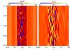 |
Fig. 8 Vertical slice of the elliptically unstable vortex core showing vertical vorticity (left panel) and vertical velocity (right panel). The motion in the core constitutes a subsonic turbulence at maximum speeds reaching 10% that of sound. |
4.1. Magnetic fields. Interaction of the MRI and the BI
The baroclinic instability demonstrated in the past sections seems to be able to drive angular momentum transport in accretion disks. As such, it could be thought of as an alternative to the MRI. Nevertheless, an important question to ask is how the two instabilities interplay. What happens if a magnetic field is introduced into the simulation?
To answer this question, we take a snapshot of the quantities at 200 orbits, and add a
constant vertical magnetic field to it, of strength
B = 5 × 10⁻³ (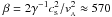 ). We assume ideal MHD, i.e. perfectly
coupling of the field to the gas (run P in Table 2). The same setup in a barotropic box leads to MRI turbulence with
alpha values of the order of α ≈ 5 × 10⁻². When the field is
introduced into the MRI unstable box, the Maxwell stress immediately starts to grow,
saturating after ≈ 3 orbits, as expected from the MRI. The Reynolds stress due to the MRI
supersedes the stresses due to the BI by one order of magnitude (see Fig. 9). The pattern is the same as with an MRI-only box. The
conclusion is immediate: the BI plays little or no role in the angular momentum transport
when magnetic fields are well-coupled to the gas. This was intuitively expected, since the
BI has weak angular momentum transport, as well as slow growth rates. The MRI is faster by
1 order of magnitude and much stronger.
). We assume ideal MHD, i.e. perfectly
coupling of the field to the gas (run P in Table 2). The same setup in a barotropic box leads to MRI turbulence with
alpha values of the order of α ≈ 5 × 10⁻². When the field is
introduced into the MRI unstable box, the Maxwell stress immediately starts to grow,
saturating after ≈ 3 orbits, as expected from the MRI. The Reynolds stress due to the MRI
supersedes the stresses due to the BI by one order of magnitude (see Fig. 9). The pattern is the same as with an MRI-only box. The
conclusion is immediate: the BI plays little or no role in the angular momentum transport
when magnetic fields are well-coupled to the gas. This was intuitively expected, since the
BI has weak angular momentum transport, as well as slow growth rates. The MRI is faster by
1 order of magnitude and much stronger.
 |
Fig. 9 Angular momentum transport with only the baroclinic instability in a 3D run and the baroclinic and magneto-rotational instabilities, after 200 orbits. The pattern after including the magnetic field is equal to that generated by MRI-only, from which we conclude that the BI is irrelevant if magnetic fields are well-coupled to the gas. |
In Fig. 10 we show the evolution of energies, enstrophy, and temperature, before and after including the magnetic field (at 200 orbits). The magnetic energy behaves as expected from the MRI, a fast growth and saturation after ≈ 3 orbits, with most of the energy stored in the azimuthal field. The kinetic energy of the turbulence increases by one order of magnitude and is more isotropic, also as expected from the MRI. The temperature increases by a factor of ≈ 2 in 15 orbits. This is because the MRI turbulence heated the box faster than the thermal relaxation time could bring the temperature back to T0.
With this experiment we expected to assess the possibility of synergy between the instabilities, but as far as we can tell, none is observed because the MRI alone dictates the evolution.
 |
Fig. 10 Evolution of box-average quantities (clockwise: kinetic energy, magnetic energy, enstrophy and temperature) before and after inserting the magnetic field. The MRI quickly takes over, on its characteristic short timescale. No evidence of synergy between the two instabilities is observed. The saturated state of the combined baroclinic+MRI resembles an MRI-only scenario. |
 |
Fig. 11 Evolution of vorticity (upper panels) and magnetic energy (lower panels) in 3D. As the MRI develops, the vortex is destroyed by the magnetic field. In a nonmagnetic run, the vortex survives indefinitely. |
 |
Fig. 12 Time evolution of the 1D spatial average of enstrophy (upper panels) and azimuthal magnetic field (middle panels) for the runs in Table 2. The lower panels refer to the magnetic field attained in control runs, where ξ = 0. In all runs, the field is seen to grow first in the vortex, then in the surrounding flow. This shows that the growth rates of the magneto-elliptic instability are faster than those of the MRI. Vortex destruction is apparent in these plots as loss of spatial coherence in the enstrophy plots, and occurred in all simulations. The length of the time axis is the same for all simulations, except the control run for run S. |
4.1.1. Vortex destruction by the magnetic field
If the evolution of the box-averaged quantities brings no surprises, the same cannot be said of their spatial distribution. In Fig. 11 we plot vorticity at three consecutive orbits after insertion of the magnetic field. Magnetic energy is also shown. The vortex, which in a nonmagnetic run retains its coherence indefinitely, is dilacerated when magnetic fields are included. In Fig. 12 we plot 1D spatial averages against time of the vertical enstrophy (upper panel) and magnetic energy of the azimuthal field (middle panel). A control run where ξ = 0 is also shown (lower panel). The figure also shows other simulations (discussed later). The run in question is the leftmost one, labeled “P”. It is apparent from the enstrophy plot that the vortex bulges, then gets destroyed as the magnetic energy grows.
To understand this behavior, we examined the state of the vortex prior to inserting the
field. In Fig. 13 we measure the vorticity profile
of the vortex. The figure shows a slice at the midplane, where we define a box of size
8H × 2H centered on the vorticity minimum. We used
elliptical coordinates such that the radius is  , where
χ = a/b is the vortex aspect ratio
(a is the semimajor and b the semiminor axis). The
coordinates xc and yc are
rotated by a small angle to account for the off-axis tilt of the vortex,
(xc,yc) = R(x − x0,y − y0),
where R is the rotation matrix, and
(x0,y0) are the coordinates of
the vortex center, found by plotting ellipses and looking for a best fit. We find that
χ = 4 and a rotation of 3° best fits the vortex core. Two such
ellipses are plotted in the upper panel of Fig. 13.
, where
χ = a/b is the vortex aspect ratio
(a is the semimajor and b the semiminor axis). The
coordinates xc and yc are
rotated by a small angle to account for the off-axis tilt of the vortex,
(xc,yc) = R(x − x0,y − y0),
where R is the rotation matrix, and
(x0,y0) are the coordinates of
the vortex center, found by plotting ellipses and looking for a best fit. We find that
χ = 4 and a rotation of 3° best fits the vortex core. Two such
ellipses are plotted in the upper panel of Fig. 13.
We then measured the vertical vorticity within the box, averaged all vertical
measurements for a given radius, and box-plotted the z-averaged
measurements against rV. The box plot uses
a bin of ΔrV = 0.01. The result is seen in
the lower panel of Fig. 13, with the radius of the
ellipses drawn in the upper panel. It is seen that the vortex core (inside the inner
ellipse) has a vorticity profile that is well approximated by a Gaussian,
 , where
ω0 = 0.62, r0 = 0.1, and the
radii are in elliptical coordinates.
, where
ω0 = 0.62, r0 = 0.1, and the
radii are in elliptical coordinates.
 |
Fig. 13 Vorticity profile of the vortex, prior to the insertion of the magnetic field. We measure the vertical vorticity in the midplane of the simulation against the elliptical radius, in the grid points boxed by the thin black line as shown in the upper panel. The modulus of the vorticity is plotted in the lower panel. The conclusion is that the vortex core has an angular velocity profile close to uniform, with shear where it couples to the Keplerian flow. The dashed lines in the lower panel mark the position of the dotted ellipses in the upper panel. They have an aspect ratio χ = 4, and mark elliptical radii of rV = 0.065 and rV = 0.13. The inner one encloses the vortex core. |
We conclude that the vorticity in the core is close to uniform (as a Gaussian is very flat near the peak amplitude). Because the vorticity is finite and close to uniform, so is the angular momentum, and thus little radial shear should be present in the core. As the MRI feeds on shear, one can expect that a patch of constant (or nearly constant) angular momentum should be stable. Nevertheless, examining the vorticity after 2 orbits of the insertion of the field, (upper middle panel of Fig. 11), we notice that the core did become unstable. This seems to be a signature of the magneto-elliptic instability (Lebovitz & Zweibel 2004; Mizerski & Bajer 2009), which we consider in the next section.
4.1.2. Magneto-elliptic instability
The elliptic instability has been a topic of extensive study in fluid mechanics (see review by Kerswell 2002). First studied in the context of absent background rotation (Bayly 1986; Pierrehumbert 1986), the effect of the Coriolis force was studied by Miyakazi (1993), followed by the effect of magnetic fields by Lebovitz & Zweibel (2004). The general case, in which both background rotation and magnetic fields are present, has recently been studied by Mizerski & Bajer (2009).
These studies have unveiled two regimes of operation, which may as well be seen as two different instabilities. The first de-stabilization mechanism is through resonances between the frequency of inertial waves and harmonics of the vortex turn-over frequency. This instability is three-dimensional, existing for θ > 0 (the angle θ being the angle between the wavevector of the pertubations and that of the vortex motion). Lebovitz & Zweibel (2004) show that this instability persists in the presence of magnetic fields, and that its effect is twofold. While it lowers the growth rates of the elliptically unstable modes, the excitation of MHD waves allows for de-stabilization of whole new families of resonances.
The second destabilizing mechanism occurs only when the Coriolis force is included (Miyakazi 1993). This instability is nonresonant in nature and exists only for θ = 0 modes, i.e., oscillations in the same plane of the motion of the vortex. Because this plane is associated with a “horizontal” (xy) plane (thus kz modes), this destabilizing mechanism has been called “horizontal instability”. As shown by Lesur & Papaloizou (2009), this nonresonant instability results in exponential drift of epicyclic disturbances. It can thus be regarded as an analog of the Rayleigh instability, but for elliptical streamlines. For a vortex embedded in a Keplerian disk, the modified epicylic frequency goes unstable for the range of aspect ratios 3/2 < χ < 4.
Mizerski & Bajer (2009) present the analysis
of the general case, including both the Coriolis and Lorentz forces. They confirm the
previous effects of the Coriolis and Lorentz forces in isolation, and find that the
horizontal instability, when present, dominates over all other modes. They also find
that the magnetic field widens the range of existence of the horizontal instability to
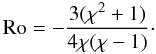
an unbounded interval of aspect ratios when 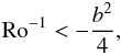 (15)where
 (16)is the Rossby number,
 (17)is another measure of the ellipticity, and
 (18)is a dimensionless parametrization of the
magnetic field, with k the wavenumber. We can also write
b = q/Ro, where
(18)is a dimensionless parametrization of the
magnetic field, with k the wavenumber. We can also write
b = q/Ro, where
 (19)is a more usual dimensionless
parametrization of the magnetic field, based on the Balbus-Hawley wavelength
λBH = 2πvA/ΩK
(Balbus & Hawley 1991; Hawley & Balbus
1991). The analysis of Mizerski & Bajer
(2009) also assumes that the vortex is of the
type
(19)is a more usual dimensionless
parametrization of the magnetic field, based on the Balbus-Hawley wavelength
λBH = 2πvA/ΩK
(Balbus & Hawley 1991; Hawley & Balbus
1991). The analysis of Mizerski & Bajer
(2009) also assumes that the vortex is of the
type  (20)When there is a magnetic field but the
criterion posed by Eq. (15) is not
fulfilled, Mizerski & Bajer (2009) find that
the field has an overall stabilizing effect on the resonant modes of the classical
(hydro) elliptic instability.
(20)When there is a magnetic field but the
criterion posed by Eq. (15) is not
fulfilled, Mizerski & Bajer (2009) find that
the field has an overall stabilizing effect on the resonant modes of the classical
(hydro) elliptic instability.
We can rewrite Eq. (15) in more
familiar terms by isolating the wavenumber and expressing the criterion in terms of
ΩK and Ro  (21)We estimate the Rossby number of the vortex
in Fig. 13. Assuming the elliptic flow of
Eq. (20), the vorticity is
ωT = 2δΩV.
The subscript T stands for “total”. This distinction is necessary because the sheared
flow amounts to a vorticity of
ωbox = − 3ΩK/2.
The total vorticity is
ωT = ωV + ωbox,
where ωV is the vortex’s intrinsic
vorticity. By isolating
ΩVδ and dividing by
ΩK, we have
(21)We estimate the Rossby number of the vortex
in Fig. 13. Assuming the elliptic flow of
Eq. (20), the vorticity is
ωT = 2δΩV.
The subscript T stands for “total”. This distinction is necessary because the sheared
flow amounts to a vorticity of
ωbox = − 3ΩK/2.
The total vorticity is
ωT = ωV + ωbox,
where ωV is the vortex’s intrinsic
vorticity. By isolating
ΩVδ and dividing by
ΩK, we have
 (22)In the absence of a vortex, the Rossby
number is still finite, Ro = − 3/4, because of the vorticity of the shear flow. In this
limit, Eq. (21) becomes
(22)In the absence of a vortex, the Rossby
number is still finite, Ro = − 3/4, because of the vorticity of the shear flow. In this
limit, Eq. (21) becomes
 which is the criterion for the MRI (Balbus
& Hawley 1991). As we shall see, the growth
rate in this limit also matches that of the MRI. This suggests that the MRI is a
particular case of the magneto-elliptic instability.
which is the criterion for the MRI (Balbus
& Hawley 1991). As we shall see, the growth
rate in this limit also matches that of the MRI. This suggests that the MRI is a
particular case of the magneto-elliptic instability.
 |
Fig. 14 Shear as the common ground between the magneto-rotational and magneto-elliptical instabilities. The distance between two points in uniform rotation does not increase if the streamlines are circular, i.e., the rotation is rigid (upper figure). However, in elliptic streamlines the distance between the two points does increase even if the rotation is uniform (lower figure). A magnetic field connecting the two points will resist this shear, leading to instability depending on the field strength. |
Since we measured
ωV/ΩK ≈ − 0.6,
the Rossby number is approximately Ro ≈ − 1. These results are compatible with the Kida
solution (Kida 1981)
 (23)from which we derive
 (24)and thus
 (25)For \begin{formule}$\chi = 4$\end{formule},
the expressions above yield
ωV/ΩK = −5/8 = −0.625,
which matches well the vorticity plateau measured in Fig. 13, and Rossby number Ro = −17/16 ≈ −1. Since the Rossby number is Ro ≈ −1,
Eq. (21) implies that the horizontal
instability in the vortex is present when q ≲ 2.
(25)For \begin{formule}$\chi = 4$\end{formule},
the expressions above yield
ωV/ΩK = −5/8 = −0.625,
which matches well the vorticity plateau measured in Fig. 13, and Rossby number Ro = −17/16 ≈ −1. Since the Rossby number is Ro ≈ −1,
Eq. (21) implies that the horizontal
instability in the vortex is present when q ≲ 2.
In dimensionless units, we use Lz = 0.2, and a resolution of Nz = 128 points in the z-direction, so the wavenumbers present in the box are k0 < k < kNy, where k0 = 2π/Lz = 31 is the largest scale, and kNy = π/Δz = 2011 is the Nyquist scale. The Pencil Code needs eight points to resolve a wavelength without significant numerical dissipation, so for practical purposes, the maximum wavenumber of the inertial range is kNy/4 = 503. Also in dimensionless units, μ0 = ρ0 = ΩK = 1, so for B0 = vA = 5 × 10⁻³, the condition posed by Eq. (21) is k < 400, well within the range captured by our box.
As for growth rates, Mizerski & Bajer (2009) do not unveil a simple expression. The solution has to be computed numerically3. The growth rate is a function of χ, q, and the angle θ between the z-axis and the wavevector of the perturbation. Technically, the Rossby number is also a free parameter, but the Kida solution ties the Rossby number to the aspect ratio. We present the growth rates for χ = 4 in the q-θ plane in the left panel of Fig. 15.
 |
Fig. 15 Left. Numerically calculated growth rates of the
magneto-elliptic instability for elliptic streamlines of aspect ratio
χ = 4 as a function of the dimensionless magnetic field
strength
q = kvA/ΩK
and the angle θ between the wavevector of disturbances and the
vertical axis. Pure kz modes are the
most unstable ones, having a critical wavelength near the predicted
|

It is seen that the most unstable modes are those of the horizontal instability (θ = 0, or kz modes). The right panel of Fig. 15 shows the growth rates of these modes for a series of aspect ratios. For χ = 2 and χ = 3, we are in the range of existence of the classical (hydro) horizontal instability, noted by the fact that fast exponential growth exists for vA = 0. For χ = 4 onwards, the instability does not exist or is too weak in the hydro regime, and the most unstable wavelength is found in the vicinity of q = 1. Although a critical wavelength exists for kz modes, 3D resonant instability exists for an unbounded range of wavenumbers, albeit with slower growth rates. In the next sections, unless otherwise stated, whenever we mention “magneto-elliptic instability” we mean the horizontal, nonresonant, magneto-elliptic modes.
We also calculate the growth rate in the limit of pure shear flow, which we approximate
numerically by χ = 100. In this case, there are no 3D unstable modes,
since there is no finite vortex turnover frequency to establish resonances. The only
instability present is horizontal (kz),
which we also show in the right panel of Fig. 15.
The critical wavelength is  , most unstable wavelength
q ≈ 1, with growth rate
σ ≈ 0.75ΩK. One
immediately recognizes that these properties are the properties of the MRI. That the MRI
is a limiting case of the magneto-elliptic instability makes sense because Eq. (20) with the Kida solution reduce to a
Keplerian sheared flow when χ tends to infinity. Physically, the
destabilization of kz modes of the elliptic
and magneto-elliptic instability mean exponential drift of epicyclic disturbances. The
equivalent of epicyclic disturbances for χ → ∞ are radial perturbations
in a sheared flow. The magneto-rotational and magneto-elliptic are in essence the same
instability. Another way of seeing the common ground between the instabilities is by
realizing that, although constant angular momentum means rigid rotation in circular
streamlines, it does not mean so when it comes to elliptical streamlines. Figure 14 illustrates this point. The length of a line
connecting two points is conserved in uniform circular motion, but not in uniform
elliptical motion4. In other words, uniform
elliptical motion contains shear. A magnetic field connecting the two points will resist
that shear, leading to instability depending on the field strength.
, most unstable wavelength
q ≈ 1, with growth rate
σ ≈ 0.75ΩK. One
immediately recognizes that these properties are the properties of the MRI. That the MRI
is a limiting case of the magneto-elliptic instability makes sense because Eq. (20) with the Kida solution reduce to a
Keplerian sheared flow when χ tends to infinity. Physically, the
destabilization of kz modes of the elliptic
and magneto-elliptic instability mean exponential drift of epicyclic disturbances. The
equivalent of epicyclic disturbances for χ → ∞ are radial perturbations
in a sheared flow. The magneto-rotational and magneto-elliptic are in essence the same
instability. Another way of seeing the common ground between the instabilities is by
realizing that, although constant angular momentum means rigid rotation in circular
streamlines, it does not mean so when it comes to elliptical streamlines. Figure 14 illustrates this point. The length of a line
connecting two points is conserved in uniform circular motion, but not in uniform
elliptical motion4. In other words, uniform
elliptical motion contains shear. A magnetic field connecting the two points will resist
that shear, leading to instability depending on the field strength.
Judging from the Fig. 15, the growth rates of the
magneto-elliptic instability at the Balbus-Hawley wavelength q = 1 seem
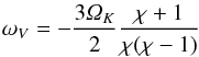
to be well-reproduced by a fit  (26)i.e., scaled by a factor
(χ + 1)/χ with respect to those of the MRI. We
hereafter refer to this χ = 100 ≫ 1 curve as the MRI limit.
(26)i.e., scaled by a factor
(χ + 1)/χ with respect to those of the MRI. We
hereafter refer to this χ = 100 ≫ 1 curve as the MRI limit.
4.2. Isolating the vortex magnetic action
As seen in Fig. 15, the wavelength range of the magneto-rotational and (horizontal) magneto-elliptic instabilities are almost the same for the aspect ratio of interest, leaving only a narrow range where one instability is captured but not the other. However, the growth rates differ, and we can explore this fact. The maximum growth rate for χ = 4 is σ ≈ 0.95ΩK. While the MRI is amplified a millionfold in three orbits, the magneto-elliptic instability is amplified by more than a billionfold in the same time interval. We study in this section limiting cases where the instabilities do not grow as fast as in Fig. 11, thus allowing us to better study their behavior. Because the magneto-rotational and magneto-elliptic instabilities will both be present in the simulations, we loosely refer to them collectively as “the MHD instabilities” or just “the instabilities” in the next sections.
4.2.1. Increasing the field strength – Stabilization of elliptic instability and channel flows
We add to the box a vertical field of strength
Bz = 6 × 10⁻². Since the
smallest wavenumber of the box is k0 = 31, we have that the
critical wavenumber for the MRI is
k/k0 = 0.9 and thus the box is MRI-stable.
The critical wavenumber for the magneto-elliptic instability, according to Eq. (21), is
k/k0 = 1.13 and thus in principle
resolved. We aim with this to explore the window between
 where the MRI is suppressed but not the
horizontal magneto-elliptic instability.
where the MRI is suppressed but not the
horizontal magneto-elliptic instability.
We follow the evolution of box-average quantities in Fig. 16. The run in question is shown in that plot as green dot-dot-dot-dashed lines, and corresponds to run Q1 in Table 2.
After insertion of the field, we immediately see a decrease in the box average of the vertical velocities. The vertical vorticity is unchanged. Radial and azimuthal fields decay with the decay of the vertical velocity. A weak vertical magnetic field of rms β = 1000 is sustained. Even though the analysis provides an elliptical wavelength that is shorter than the box length, we do not seem to witness a magneto-elliptic instability in operation. In fact, we are in the range of stable Rossby numbers, evidence of which is that the elliptic instability was stabilized after inserting the field. This is not really worrisome considering that the derived critical wavenumber was so close to k0, and we made some approximations. It is curious, though, that we do not see growth in the unstable resonant modes. For wavelengths emcompassing the vortex core (λy = 2H or λx = H/2; each of them well-resolved with 32 points), the maximum growth rate is at the vicinity of σ = 0.33ΩK, yielding a millionfold amplification in less than 7 orbits. We ran this simulation for 30 orbits after inserting the field. At present, we can offer no explanation as to why these modes did not become unstable.
We also test a run with a slightly less strong field, Bz = 3.75 × 10⁻² (run Q2). In that case, the magneto-rotational and magneto-elliptic instabilities have critical wavelengths of k/k0 = 1.47 and k/k0 = 1.78, respectively, so both instabilities ought to be resolved. The largest scale of the box corresponds to q = 1.18, close to the maximum growth rate of both instabilities. The magneto-elliptic instability has a faster growth rate, so it should be seen first.
What we witness is quite revealing. The vortex is destroyed in 4 orbits, while the MRI is still growing in the box. A growth of magnetic energy occurs within the vortex at a very fast pace. The vortex is destroyed when still in the phase of linear growth of the instability, owing to the development of a conspicuous and strong channel flow (Fig. 17). Because the flow in different layers occurs in different directions, the vortex is stretched apart and loses its vertical coherence.
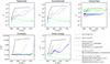 |
Fig. 16 Isolating the vortex magnetic action. The lines show the magnetic runs with the MHD instabilities (magneto-elliptic and magneto-rotational) resolved in ideal MHD (P, black solid); unresolved with strong field (Q1, green dot-dot-dot-dashed); most unstable wavelength under-resolved with weak field (R, red dashed); and quenched with resistivity (S, blue dot-dashed). The nonmagnetic 3D hydro run is shown as dotted line in the lower panels. Run Q1 shows that strong magnetic fields have a stabilizing effect on the elliptical instability. Run R shows the magneto-elliptic instability seeming to saturate (at 203 orbits) before the MRI takes over (at 207 orbits). In runs Q2 and S2, the vortex survives until a channel flow develops in the box. |
We notice that, prior to the excitation of the channel flow, the elliptical instability in the core was suppressed, which is also obvious from comparing the snapshots at t = 200 and 201 orbits at Fig. 17.
The run is also shown in Fig. 12 (run Q). We see that the growth of magnetic energy occurs earlier in the vortex when compared to the surrounding flow, as expected.
4.2.2. Decreasing the field strength – vortex MHD turbulence
 |
Fig. 17 The effect of a strong unstable vertical magnetic field in the vorticity column. The field is added at t = 200. At first, the effect of the field is to stabilize the elliptic turbulence, which is seen in the subsequent snapshots. The disappearance of the vortex at later times is caused by the development of a strong channel flow that stretches the column and destroys its vertical coherence. If the initial vertical field is stable, the strength of the channel does not grow and the vortex survives indefinitely. |
Next we checked the behavior of the flow by adding weak magnetic fields. The goal was to slow the MHD instabilities by not resolving their most unstable wavelengths, q ≈ 1. Both instabilities thus operate at a slower pace, which results in stretching the time interval while one (magneto-elliptic in the vortex) is saturating and the other (magneto-rotational in the box) still growing.
 |
Fig. 18 Time series of enstrophy and plasma beta for run R, where the instabilities grow at lower growth rates than in run P (Fig. 11). The magneto-elliptic instability grows faster than the MRI, which is seen as the strong turbulence that develops in the core, while the underlying Keplerian flow is still laminar. Once the MRI saturates, the strain of its turbulence destroys the vortex spatial coherence. It is not conclusive if the vortex would have survived the magneto-elliptic instability had the MRI not destroyed it first. |
 |
Fig. 19 Time series of enstrophy and plasma beta for runs S, where the instabilities are quenched with resistivity. The upper panels correspond to a high-resistivity run, where even the longest wavelength of the box is damped. The simulation is similar to a nonmagnetized run, the vortex surviving indefinitely. In the lower panels we used lower resistivity with Elsässer number Λ = 1. The longest wavelength of the box thus has a magnetic Reynolds number of 6, so its growth is not quenched. The magneto-elliptic instability grows in the vortex core in a conspicuous kz/k0 = 2 mode. Part of the field generated is diffused away due to the high resistivity. Channel flows eventually develop, destroying the vortex. |
The cell size in the z-direction is 1.6 × 10⁻³. We add a field of strength Bz = 1.5 × 10⁻³. The Balbus-Hawley wavenumber is kBH = 667, and thus resolved but within the viscous range. The first properly resolved wavenumber is k ≈ 500, which corresponds to q ≈ 0.75. The run is shown in Fig. 16 as dashed red line, and labeled R in Table 2 and Fig. 12.
It is seen that the MRI in the Keplerian flow is suppressed, yet an instability is present. We identify it with the magneto-elliptic instability, as it coincides with the vortex core going unstable, as shown in the snapshots of Fig. 18.
The vortex is magneto-elliptic unstable, yet it does not seem to lose its spatial coherence. The magnetic field is mostly confined to the vortex, which shows as a region of high Alfvén speeds, when the surrounding Keplerian flow is still laminar. The instability is violent, making the vortex bulge. This is apparent in Fig. 18 as the vortex seems to have grown radially from t = 203 to t = 206 orbits. During this period, however, the box average of kinetic energy and enstrophy are nearly constant (Fig. 16), so it is not clear if this magneto-elliptic turbulence would have led to vortex destruction, or if it would have reached a steady state. The process just outlined is well-illustrated in Fig. 12 (run R). One orbit later, the MRI starts to develop in the surrounding Keplerian flow (notice the difference between these time scales and those of Fig. 11), which corresponds to the increase in box-average quantities in Fig. 16 at that time. No strong channel flow is excited. The level of vorticity due to the MRI is nonetheless bigger than that of the vortex. The latter eventually becomes inconspicuous in the midst of the box turbulence.
We also tested a weaker field, of strength
Bz = 6 × 10⁻⁴. The wavenumbers
of the analysis above were then scaled by 2.5, so the first resolved wavenumber
corresponds to q = 0.3. In this case, no significant action was seen.
After ten orbits, the intensity of the magnetic energy was only 4 × 10⁻⁹,
accompanied by a merely slight increase in the kinetic energy of the vertical velocities
( and
and
 remained unchanged). The minimum plasma
beta was still as high as 104.
remained unchanged). The minimum plasma
beta was still as high as 104.
4.2.3. Resistivity
To test the last case, we used a resistivity high enough that the longest unstable wavelength present in the box has a magnetic Reynolds number of unity. This wavelength is of course Lz, the vertical length of the box. The resistivity then is such that ReM = LzvA/η = 1; for a field of strength Bz = 5 × 10⁻³, this magnetic Reynolds number corresponds to η = 10-3. This is the same field that was used in the fiducial MHD run (Fig. 11), of kBH = 200, so the instabilities are resolved in the absence of resistivity. The run is labeled S in Table 2. The results are shown in the upper panels of Fig. 19.
The simulation is not very different from a purely hydro run. The damped magnetic field only has a slight stabilizing effect on the elliptical instability. A slight amount of the kinetic energy of the core turbulence gets converted into magnetic energy, which then diffuses away. The vortex becomes, at later times, less magnetized than the surroundings.
The situation should change when the resistivity is lowered slightly, allowing some
unstable wavelengths to have ReM > 1, yet still quenching
the most unstable wavelengths. For that, we set the Elsässer number to
 . The Elsässer number is equivalent to
the magnetic Reynolds number
ReM = LU/η taking the
length L as the MRI wavelength, and velocity U as the
Alfvén velocity. As such, it is the quantity governing the behavior of the MRI (e.g.,
Pessah 2010). Having Λ=1 corresponds to
. The Elsässer number is equivalent to
the magnetic Reynolds number
ReM = LU/η taking the
length L as the MRI wavelength, and velocity U as the
Alfvén velocity. As such, it is the quantity governing the behavior of the MRI (e.g.,
Pessah 2010). Having Λ=1 corresponds to
 , or
η ≃ 1.6 × 10⁻⁴ in dimensionless units. The magnetic
Reynolds number of the longest wavelength is thus ≈ 6. The results are shown in the
lower panels of Fig. 19.
, or
η ≃ 1.6 × 10⁻⁴ in dimensionless units. The magnetic
Reynolds number of the longest wavelength is thus ≈ 6. The results are shown in the
lower panels of Fig. 19.
The vertical field again has a stabilizing effect on the elliptical turbulence. This is seen as a weakening of the vertical kinetic energy in Fig. 16, which lasts for two orbits. The difference between this run and the more resistive one is that thanks to the excitation of magneto-elliptic modes, radial and azimuthal fields grow inside the vortex core, and a conspicuous k/k0 = 2 vertical mode appears (lower panels of Fig. 19). The field gets looped around the vortex, initially making the vorticity patch a region of higher Alfvén speeds. Owing to the high resistivity, however, the field diffuses away (the time for the field to diffuse over a scale height is t = H2/η ≈ 10 orbits). The radial field gets sheared into azimuthal by the Keplerian flow. After a few orbits, strong magnetic fields are seen in the vortex spiral waves. At later times, the exponential growth of radial and azimuthal fields, as well as the excited z-velocities, are seen in these waves. This process is illustrated in Fig. 20.
A look at the induction equation illustrates the process. Under incompressibility and
elliptical motion (Eq. (20)), the
equations for the in-plane field perturbations under the influence of a vertical
magnetic field and resistivity are 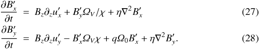 The first term in both equations generates
field out of velocity perturbations. This is the only source term for the in-plane
field. Under waning velocity perturbations, the generation of fields dies out as well.
The second term is also stretching, but under the vortical motion, thereby turning
radial fields into azimuthal and vice-versa, at the vortex frequency. Its effect is to
wrap around the vortex the fields generated by the first term. The field then diffuses
away due to the resistivity. The radial field is sheared into azimuthal because of the
third term in the azimuthal field equation.
The first term in both equations generates
field out of velocity perturbations. This is the only source term for the in-plane
field. Under waning velocity perturbations, the generation of fields dies out as well.
The second term is also stretching, but under the vortical motion, thereby turning
radial fields into azimuthal and vice-versa, at the vortex frequency. Its effect is to
wrap around the vortex the fields generated by the first term. The field then diffuses
away due to the resistivity. The radial field is sheared into azimuthal because of the
third term in the azimuthal field equation.
In this simulation, the magnetic Reynolds number of the longest wavelength is ReM = LzvA/η = 6, so even though the most unstable wavelength of the MRI is suppressed, slower growing wavelengths are present. Since they amplify the field, strong channel flows eventually appear in the simulation. At 10 orbits the azimuthal field of the channel achieves the same strength as that of the field in the vortex. The box went turbulent at 15 orbits (Fig. 12), slightly after the destruction of the vortex by the channel flow. We note, however, that in the control run for the simulation in question, the MRI grew slower, only becoming noticeable at ≈ 20 orbits (notice the larger range of the time axis for the control run). It appears that the field produced by the magneto-elliptic instability in the vortex and then diffused to the box led to the faster growth compared to the ξ = 0 control run.
A simulation where the Reynolds number of the longest wavelength was three also shows the same qualitative behavior, albeit in longer timescales. We followed a simulation of Reynolds number two for the same time, and no growth was seen. The timescale for growth in this case may be infinite (stable) or just impractically long. We conclude that resistivity suppresses the magneto-elliptic instability when the longest unstable wavelength has a magnetic Reynolds number of the order of unity, as intuitively expected.
 |
Fig. 20 Time series of enstrophy and azimuthal field in the midplane for run S2, of moderate resistivity. By action of the magneto-elliptic instability, the field initially grows inside the vortex. Due to the resistivity, it then diffuses away from the vortex, coupling to the waves excited by it. At later times, exponential growth of the field is seen in the wake. The vortex itself appears unmagnetized. |
4.3. Constant azimuthal field and zero net flux field
The analysis of the magneto-elliptic instability by Mizerski & Bajer (2009) was done for a system thread by a uniform constant magnetic field. We seek here to establish the effect of a zero-net flux field. As it turns out, the vortex is quite unstable to such configurations as well.
We add a field whose initial value is  , where
k0z = 2π/Lz,
and B0 = 10-2. The run is labeled
U in Table 2 and Fig. 12. The most unstable wavelength for the MRI has
k = 100, hence well-resolved. In a barotropic box, this field led to
saturated turbulence after 3 orbits. The critical wavelength for the magneto-elliptic
instability has k = 200, also well resolved. As shown in Fig. 12, the vortex becomes unstable well before the box
turbulence starts. In 1 orbit after insertion of the field, the vortex column has already
lost its coherence.
, where
k0z = 2π/Lz,
and B0 = 10-2. The run is labeled
U in Table 2 and Fig. 12. The most unstable wavelength for the MRI has
k = 100, hence well-resolved. In a barotropic box, this field led to
saturated turbulence after 3 orbits. The critical wavelength for the magneto-elliptic
instability has k = 200, also well resolved. As shown in Fig. 12, the vortex becomes unstable well before the box
turbulence starts. In 1 orbit after insertion of the field, the vortex column has already
lost its coherence.
As for an azimuthal field, Kerswell (1994) studied
the effect of toroidal field on elliptical streamlines, finding only a slight stabilizing
adjustment of the growth rates of the elliptical instability. The analysis, however, only
holds for the limit of nearly circular streamlines (χ → 1). Given the
stark difference in the behavior of vertical fields in different configurations, there is
reason to believe the same should apply to azimuthal fields. We add a field
 , with
B0 = 0.03 (run T in Table 2). Once again, the vortex is quickly destroyed, as
seen in Fig. 12.
, with
B0 = 0.03 (run T in Table 2). Once again, the vortex is quickly destroyed, as
seen in Fig. 12.
5. Conclusions
We model for the first time the evolution of the baroclinic instability in 3D including compressibility and magnetic fields. We find that the amount of angular momentum transport due to the inertial-acoustic waves launched by unmagnetized vortices is at the level of α ≈ 5 × 10⁻³, positive, and compatible with the value found in 2D calculations.
When magnetic fields are included and well-coupled to the gas, an MHD instability destroys the vortex in short timescales. We find that the vortices display a core of nearly uniform angular velocity, as claimed in the literature (e.g., Klahr & Bodenheimer 2006), so this instability is not the MRI. We identify it with the magneto-elliptic instability studied by Lebovitz & Zweibel (2004) and Mizerski & Bajer (2009).
Though Lebovitz & Zweibel (2004) report that the magneto-elliptic instability has lower growth rates than the MRI, our simulations show the vortex core going unstable faster than the box goes turbulent. That is because the presence of background Keplerian rotation allows for destabilization of kz modes (horizontal instability), which have higher growth rates. We also show that the stability criterion and growth rates for the magneto-elliptic instability derived by Mizerski & Bajer (2009), when taken in the limit of infinite aspect ratio (no vortex) and with shear, coincide with those of the MRI. Both instabilities have a similar most unstable wavelength, yet the growth rates of the magneto-elliptic instability in the range of aspect ratios 4 < χ < 10 are approximately 3 times faster than for the MRI.
After the vortex is destroyed, the saturated state of the MRI+BI simulation resembles an MRI-only simulation. The same box-averaged values of α, enstrophy, kinetic, and magnetic energies are measured in the two cases. The conclusion is that the background entropy gradient plays only a small role when magnetic fields are present and well-coupled to the gas. The enstrophy produced by the BI is four orders of magnitude lower than that produced by the MRI.
We performed a series of numerical experiments to determine the behavior of the magneto-elliptic instability in limiting cases. First, we increased the field so that the critical MRI wavelength is bigger than the box. In that case, the elliptical turbulence dies out almost immediately after inserting the field. We take it as evidence of the stabilizing effect of strong magnetic fields on the classical (hydro) elliptical instability. When the field is slightly decreased so that some unstable wavelengths are resolved, the magnetic field inside the vortex core grows rapidly, leading to channel flows that soon break the spatial coherence of the vortex column.
Second, we slow down the instabilities to better study the magneto-elliptic instability in isolation. Decreasing the growth rate by a factor x stretches the time period between their saturations by the same factor. We thus decreased the field so that the most unstable wavelength in the box is underresolved. In this case, we witness the development of magneto-elliptic turbulence in the vortex core only. This turbulence was violent, but it is not clear if it would have led to destruction of the vortex. After seven orbits, longer MRI-unstable wavelengths in the box led to turbulence. The vortex was destroyed by the strain of that turbulence, bulging and losing coherence, and was eventually lost in the turbulent vorticity field of the box. Decreasing the field further led to quenching of the magneto-elliptic instability as well.
Third, the instabilities were suppressed with physical resistivity, setting the Elsässer number to unity. In this case, there is a slight decrease in the kinetic energy of the elliptic turbulence, which lasts for two orbits. Meanwhile, in-plane magnetic fields develop inside the vortex, loop around it, and get diffused away. Vortex destruction happens when longer wavelengths in the box, for which the magnetic Reynolds number is bigger than one, go MRI-unstable. Channel flows develop, and the vortex is stretched apart. By increasing the resistivity, the instabilities are quenched when the longest wavelength of the box has a magnetic Reynolds number ReM ≲ 2.
In addition to uniform vertical fields, we also performed simulations with azimuthal fields and vertical zero net flux fields. These different field configurations also led to magneto-elliptic instability in the vortex.
In view of these results, it is curious that the vortex seen in the zero net flux MRI simulations of Fromang & Nelson (2005) is stable over hundreds of orbits, a fact left without explanation to date. We speculate that this may come from a lack of resolution in the global simulation to capture the magneto-elliptic modes in the core.
We conclude that the baroclinic instability is important only when magnetic fields are too weakly coupled to the gas. Otherwise they are destroyed by the magneto-elliptic instability, channel flows, or by the strain of the surrounding MRI turbulence. We thus underscore that our results fit neatly in the general picture of the layered accretion paradigm in protoplanetary disks. If the MRI supersedes the BI, it thus remains the main source of turbulence in the active zones where ionization is abundant. The active layers are unmodified, whereas the dead zone, if baroclinic unstable, is endowed with large-scale vortices and an associated weak but positive accretion rate of α ≈ 5 × 10⁻³. This value has to be revised by global simulations in view of the limited spatial scale of the shearing box. If confirmed, it might be sufficient for a steady state to be achieved (Terquem 2008), as long as the borders of the dead zone are stable (Lyra et al. 2009). It remains to be studied what the conditions are when vertical stratification is included, what the precise transition is between a BI dominated dead zone and the MRI-active radii/layers, and how the accumulation of solids will proceed inside elliptically turbulent vortex cores.
Actually, this is such a useful insight that some authors prefer to define entropy as S = p/ργ. The reader should then keep in mind that what we call entropy is actually s = cVln(S/S0) in that definition. Here we prefer to use the definition Eq. (7) as it comes from thermodynamics; i.e., Tds = de + pdv, where e = cVT is the internal energy and v = 1/ρ. It also enables the Brunt-Väisälä frequency to be written in a more compact form (Eq. (8)).
A script to calculate the growth rates was kindly provided by Mizerski.
As pointed out by the referee, this is clearly seen when one writes the shear stress Ssh = ∂xuy + ∂yux and substitutes the Kida solution. It yields Ssh = − ΩV(χ2 − 1)/χ, which is only zero for χ = 1.
Acknowledgments
Simulations were performed at the PIA cluster of the Max-Planck-Institut für Astronomie. We acknowledge useful discussions with K. Mizerski, C. McNally, J. Maron, M.-M. Mac Low, G. Lesur, and A. Johansen. The authors thank the anonymous referee for the many comments that helped improve the manuscript.
References
- Balbus, S., & Hawley J. 1991, ApJ, 376, 214 [NASA ADS] [CrossRef] [Google Scholar]
- Bayly, B.J. 1986, PhRvL, 57, 2160 [Google Scholar]
- Fromang, S., & Nelson, R. P. 2005, MNRAS, 364, 81 [Google Scholar]
- Gammie C. F. 1996, ApJ, 457, 355 [NASA ADS] [CrossRef] [Google Scholar]
- Hawley, J. F., & Balbus, S. A. 1991, ApJ, 376, 223 [NASA ADS] [CrossRef] [Google Scholar]
- Heinemann, T., & Papaloizou, J. C. B. 2009, MNRAS, 397, 64 [Google Scholar]
- Johnson, B. M., & Gammie, C. F. 2005, ApJ, 635, 149 [NASA ADS] [CrossRef] [Google Scholar]
- Johansen, A., Youdin, A., & Klahr, H. 2009, ApJ, 697, 1269 [NASA ADS] [CrossRef] [Google Scholar]
- Kerswell, R. R. 1994, J. Fluid Mech., 274, 194 [Google Scholar]
- Kerswell, R. R. 2002, AnRFM, 34, 83 [Google Scholar]
- Kida, S. 1981, J. Phys. Soc. Jpn, 50, 3517 [Google Scholar]
- Klahr, H. 2004, ApJ, 606, 1070 [NASA ADS] [CrossRef] [Google Scholar]
- Klahr, H. H., & Bodenheimer, P. 2003, ApJ, 582, 869 [NASA ADS] [CrossRef] [Google Scholar]
- Klahr, H., & Bodenheimer, P. 2006, ApJ, 639, 432 [NASA ADS] [CrossRef] [Google Scholar]
- Lebovitz, N., & Zweibel, E. 2004, ApJ, 609, 301 [NASA ADS] [CrossRef] [Google Scholar]
- Lesur, G., & Papaloizou, J. C. B. 2009, A&A, 498, 1 [NASA ADS] [CrossRef] [EDP Sciences] [Google Scholar]
- Lesur, G., & Papaloizou, J. C. B. 2010, A&A, 513, 60 [Google Scholar]
- Lyra, W., Johansen, A., Klahr, H., & Piskunov, N. 2008, A&A, 479, 883 [NASA ADS] [CrossRef] [EDP Sciences] [Google Scholar]
- Lyra, W., Johansen, A., Zsom, A., Klahr, H., & Piskunov, N. 2009, A&A, 497, 869 [NASA ADS] [CrossRef] [EDP Sciences] [Google Scholar]
- Mamatsashvili, G. R., & Chagelishvili, G. D. 2007, MNRAS, 381, 809 [NASA ADS] [CrossRef] [Google Scholar]
- Miyazaki, T. 1993, PhFl, 5, 2702 [Google Scholar]
- Mizerski, K. A., & Bajer, K. 2009, J. Fluid Mech., 632, 401 [NASA ADS] [CrossRef] [Google Scholar]
- Oishi, J., & Mac Low, M.-M. 2009, ApJ, 704, 1239 [NASA ADS] [CrossRef] [Google Scholar]
- Petersen, M. R., Julien, K., & Stewart, G. R. 2007a, ApJ, 658, 1236 [NASA ADS] [CrossRef] [Google Scholar]
- Petersen, M. R., Stewart, G. R., & Julien, K. 2007b, ApJ, 658, 1252 [NASA ADS] [CrossRef] [Google Scholar]
- Pierrehumbert, R. T. 1986, PhRvL, 57, 2157 [Google Scholar]
- Regev, O., & Umurhan, O. M. 2008, A&A, 481, 21 [NASA ADS] [CrossRef] [EDP Sciences] [Google Scholar]
- Shen, Y., Stone, J. M., & Gardiner, T. A. 2006, ApJ, 653, 513 [NASA ADS] [CrossRef] [Google Scholar]
- Terquem, C. E. J. M. L. J. 2008, ApJ, 689, 532 [NASA ADS] [CrossRef] [Google Scholar]
- Tevzadze, A. G., Chagelishvili, G. D., Bodo, G., & Rossi, P. 2010, MNRAS, 401, 901 [NASA ADS] [CrossRef] [Google Scholar]
- Turner, N. J., & Drake, J. F. 2009, ApJ, 703, 2152 [NASA ADS] [CrossRef] [Google Scholar]
Appendix A: Linearization of the large-scale pressure gradient
Given a pressure profile following a power law
 (A.1)we linearize it by considering
r = R0 + x, and
R0 ≫ x, as below
(A.1)we linearize it by considering
r = R0 + x, and
R0 ≫ x, as below
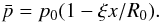 (A.2)The total pressure includes this
time-independent part, plus a local fluctuation p′
(A.2)The total pressure includes this
time-independent part, plus a local fluctuation p′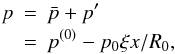 (A.3)where
  (A.4)and the superscript “(0)” denotes the part of
the pressure that has no information on the radial gradient. The pressure gradient is
therefore
(A.4)and the superscript “(0)” denotes the part of
the pressure that has no information on the radial gradient. The pressure gradient is
therefore  (A.5)The momentum equation then becomes
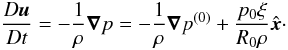 (A.6)However, this equation would not work because
it is not in equilibrium. The second term would continuously inject momentum in the box.
This is a reflection of the fact that the pressure gradient modifies the effective
gravity, and the rotation curve accordingly. In a global disk, the disk settles in
sub-Keplerian centrifugal equilibrium. We add to the equation a term that embodies this
equilibrium
(A.6)However, this equation would not work because
it is not in equilibrium. The second term would continuously inject momentum in the box.
This is a reflection of the fact that the pressure gradient modifies the effective
gravity, and the rotation curve accordingly. In a global disk, the disk settles in
sub-Keplerian centrifugal equilibrium. We add to the equation a term that embodies this
equilibrium 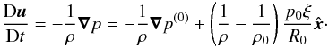 (A.7)The superscript “(0)” is dropped in
Eq. (2). The same procedure applies to
the energy equation, albeit with a small caveat, because the energy equation includes not
only the pressure gradient but also the pressure itself. In adiabatic form, the energy
equation is
(A.7)The superscript “(0)” is dropped in
Eq. (2). The same procedure applies to
the energy equation, albeit with a small caveat, because the energy equation includes not
only the pressure gradient but also the pressure itself. In adiabatic form, the energy
equation is 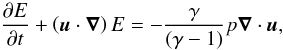 (A.8)where
E = cVρT
is the internal energy. The term on the right-hand side is the pdV work. The modifications
to the energy equation come from this term and from the radial advection term. Since
E = p/(γ − 1), and p
is given by Eq. (A.3), we have
(A.8)where
E = cVρT
is the internal energy. The term on the right-hand side is the pdV work. The modifications
to the energy equation come from this term and from the radial advection term. Since
E = p/(γ − 1), and p
is given by Eq. (A.3), we have
![Mathematical equation: \appendix \setcounter{section}{1} $$ \partial_x E = \partial_xE^{(0)} - p_0\ksi/[R_0(\gamma-1)], $$](/articles/aa/full_html/2011/03/aa15568-10/aa15568-10-eq316.png) so
so ![Mathematical equation: \appendix \setcounter{section}{1} \begin{eqnarray} \frac{\partial E^{(0)}}{\partial t} &+& \left(\v{u}\cdot\del\right) E^{(0)} = \\\nonumber &-&\frac{\gamma}{(\gamma-1)}\left[p^{(0)} - p_0\ksi\frac{x}{R_0}\right]\Div{\v{u}} + \frac{u_x p_0\ksi}{R_0(\gamma-1)}\cdot \label{eq:energy-equation} \end{eqnarray}](/articles/aa/full_html/2011/03/aa15568-10/aa15568-10-eq317.png) (A.9)We now drop the
x-dependent term in the pdV work. The main reason is because the term
is not periodic, therefore its inclusion in the shearing box can potentially lead to
long-term effects in the simulation, e.g., uneven heating due to the dissipation of waves.
It also creates a boundary in the box, and waves would be subject to refraction and
reflection upon reaching it.
(A.9)We now drop the
x-dependent term in the pdV work. The main reason is because the term
is not periodic, therefore its inclusion in the shearing box can potentially lead to
long-term effects in the simulation, e.g., uneven heating due to the dissipation of waves.
It also creates a boundary in the box, and waves would be subject to refraction and
reflection upon reaching it.
Although the discarding is not physically motivated, the loss is not as crucial as it may seem at first. This is because the term is not important for the instability cycle; that is, the pdV is not acting on the buoyancy itself. Clearly a vortical flow in geostrophic balance is divergenceless, so the pdV term is zero anyway. Thus, neglecting the x-dependent term is not affecting the baroclinic instability. If included, the term is only affecting the wave pattern, and only slightly. Waves will be subject to more heating (cooling) upon compression (expansion) on one side of the box more than the other. In fact, this could also be expressed by a radially varying adiabatic coefficient γ. A test simulation was run with the non-periodic term included, in order to assess the impact of discarding it. It was seen that the term effectively creates, over a long time, a small entropy jump in the box. Nonetheless, the development of the baroclinic instability progressed unhindered, leading to no significant different results to vortex formation. Even the large-scale sound waves have the same statistical properties. Growth rates and saturation levels of the turbulence are indistinguishable from those attained in the fiducial run.
We are of course losing consistency for dropping a term from the equations. The consistent ways of modeling the problem are either by using the Boussinesq approximation (as in Lesur & Papaloizou 2010), which filters acoustics out and eliminates the pdV term, or by means of global disk calculations, where the radial dependencies are only given in the initial condition, and are free to evolve in time. This is admittedly a limitation of the model, but the benefit of the high resolution that can be achieved in the local box, at the expense of a term that is not important for the instability cycle, was judged worth the loss in consistency.
The simplified energy equation reads as 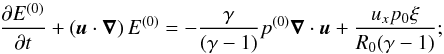 (A.10)i.e., the box has the same temperature all
over. The dependency on ux provides the
heating/cooling that a gas parcel would experience in a global model. Because of it, a gas
parcel heats up when climbing the temperature gradient, and cools down when descending it.
(A.10)i.e., the box has the same temperature all
over. The dependency on ux provides the
heating/cooling that a gas parcel would experience in a global model. Because of it, a gas
parcel heats up when climbing the temperature gradient, and cools down when descending it.
From the definition of entropy (Eq. (7)),
we write 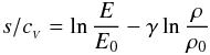 (A.11)and taking the derivative,
 (A.12)where we made use of the continuity equation.
Multiplying the whole equation by E, we have
(A.12)where we made use of the continuity equation.
Multiplying the whole equation by E, we have 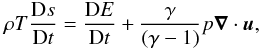 (A.13)so the pdV term cancels when converting the
energy equation into an equation for entropy. We substitute Eq. (A.10) into Eq. (A.13) to find
(A.13)so the pdV term cancels when converting the
energy equation into an equation for entropy. We substitute Eq. (A.10) into Eq. (A.13) to find
 (A.14)The superscripts “(0)” are dropped in
Eq. (7).
(A.14)The superscripts “(0)” are dropped in
Eq. (7).
Appendix B: Testing for aliasing
One critical task to perform before any attempt to quantify baroclinic growth of vorticity is to test how well the code reproduces the analytical results of shear wave theory. Compressible and incompressible modes have well-defined analytical solutions that may be used to assess the presence and quantify the amount of aliasing introduced by the scheme.
Aliasing is a feature of finite-difference codes, which occurs when a shear-wave swings from leading (kx < 0) to trailing (kx > 0). As the radial wavelength of the wave approaches zero, it becomes shorter than the width of a grid cell. The signal is lost on the Nyquist scale, and information is lost owing to the phase degeneracy that is established. There are an infinite number of possible sinusoids of varying amplitude and phase that are solutions (all “aliases” of the correct solution), so spurious power can be introduced in the wave. This extra power is then transferred from the trailing to the leading wave, which will again swing-amplify.
Because of this, it is possible that aliasing by itself may lead to spurious vortex growth. In 2D, the energy spuriously generated at the aliased swing-amplification has no option but to undergo an inverse cascade, the end of which is coherent vortices. This is a particular danger for Pencil, because the code is both finite-difference and high-order. The high-order nature is in most cases a plus, of course, since it leads to little overall numerical dissipation. In this case, however, it means that the spuriously added power will not be discarded. Lower order codes can be diffusive enough that the energy introduced by aliasing may be immediately dissipated. Indeed, Shen et al. (2006) highlight that they do not see any aliasing happening, and suggest that this is due to the high degree of numerical diffusivity in their code. This is of course a case of two negative features canceling each other.
We combine the best of both worlds by using hyperviscosity. It makes the code dissipative only where it is needed (on the grid scale), with the extra benefit of being able to control how much dissipation is added to the solution. We note that Oishi & Mac Low (2009), also using the Pencil code, tested the numerical evolution of incompressible 2D as well as compressive 2D and 3D disturbances against their analytical solutions. They found aliasing unimportant when using hyperviscosity. We repeat here the incompressible test (showed in Fig. B.1), and refer to Oishi & Mac Low (2009) and Johansen et al. (2009) for the other tests.
 |
Fig. B.1 Testing the numerical scheme for aliasing, a feature of finite difference methods, which spuriously increases the energy of a wave that swings from leading to trailing. At the resolutions and mesh-Reynolds numbers we use, this effect is successfully suppressed. The wave has a wavenumber kx,0 = − 16π/Lx, which means 4, 8, 16, and 32 points per wavelength at resolutions 32, 64, 128, and 256, respectively. The wiggling is due to excitation of compressible modes not present in the analytical solution. |
The analytical solution of the incompressible shear wave is (Johnson & Gammie 2005)
 (B.1)where
  ,
ky ≡ const., and
,
ky ≡ const., and
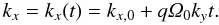 (B.2)The condition of incompressibility
\begin{formule}$k_i\delta{u_i}=0$\end{formule} thus dictates that
δuy = − kxδux/ky.
The solenoidality of the wave is guaranteed by initializing the velocity field through a
streamfunction
(B.2)The condition of incompressibility
\begin{formule}$k_i\delta{u_i}=0$\end{formule} thus dictates that
δuy = − kxδux/ky.
The solenoidality of the wave is guaranteed by initializing the velocity field through a
streamfunction  , with
 . We use the setup of Shen et al. (2006),
kx,0 = − 16π/Lx,
ky = 4π/Ly,
with
Lx = Ly = 0.5,
A = 10-4,
cs = Ω = ρ0 = 1,
γ = 7/5, and q = 3/2.
. We use the setup of Shen et al. (2006),
kx,0 = − 16π/Lx,
ky = 4π/Ly,
with
Lx = Ly = 0.5,
A = 10-4,
cs = Ω = ρ0 = 1,
γ = 7/5, and q = 3/2.
We follow the evolution of the x-velocity in a point of the grid, and
plot the result in Fig. B.1, checking for
differences due to resolution and initial mesh Reynolds number Re, defined by the
hyperviscosity coefficient  (B.3)We see that no aliasing is detected at
Re = 0.01. The signal is viscously damped before it can be swing-amplified. At Re = 0.1,
aliasing occurs at resolution 322. However, the added signal suffers a severe
(hyper-)viscous damping, so that the next swing amplification has little left to work
with. When increasing the Reynolds number to Re = 1, aliasing now happens also for
resolution 642, but the solution is decaying. Aliasing is not detected at any
Reynolds number for resolution 2562. A run with Re = ∞ for
resolution 322 (not showed) kept periodic intervals of aliasing without
dissipation but without net growth, at least until t = 1000.
(B.3)We see that no aliasing is detected at
Re = 0.01. The signal is viscously damped before it can be swing-amplified. At Re = 0.1,
aliasing occurs at resolution 322. However, the added signal suffers a severe
(hyper-)viscous damping, so that the next swing amplification has little left to work
with. When increasing the Reynolds number to Re = 1, aliasing now happens also for
resolution 642, but the solution is decaying. Aliasing is not detected at any
Reynolds number for resolution 2562. A run with Re = ∞ for
resolution 322 (not showed) kept periodic intervals of aliasing without
dissipation but without net growth, at least until t = 1000.
The panels in Fig. B.1 are for ξ = 0. When we use non-zero ξ, the aliased solutions show an increase in amplitude. The same does not happen for the solutions at low Reynolds numbers. The wiggling seen at higher resolution in Fig. B.1 is accompanied by changes in the density, which leads us to conclude that they come from the excitation of compressible modes not present in the analytical solution. We use a resolution of 2562 for 2D runs. At this resolution, we rest assured that aliasing is not happening for the considered Reynolds numbers.
All Tables
All Figures
|
Fig. 1 Snapshots of the fiducial 2D run with ξ = 2, τ = 2π, H = 0.1, and resolution 2562. A vortex is formed and establishes a local entropy gradient that counteracts the global entropy gradient that caused it in first place. Moderate cooling times keep the surfaces of constant density and constant pressure misaligned, leading to more vortex growth. In the positive feedback that ensues, giant anti-cyclonic vortices grow to the sonic scale. The initial condition was free of enstrophy. This vorticity growth was due purely to baroclinic effects. |
| In the text | |
|
Fig. 2 Left. Baroclinic enstrophy growth with thermal relaxation, where a gas parcel returns to the initial temperature on a timescale τ. A stable entropy gradient can only be maintained between the extremes of too fast a relaxation (isothermal behavior) and too slow a relaxation (adiabatic behavior). Optimal growth occurs when τ is comparable to the dynamical time. Right. Baroclinic enstrophy growth with thermal diffusion, where heat diffuses over a scale height on a timescale τ. Optimal growth occurs on longer timescales when compared to the thermal relaxation case. |
| In the text | |
|
Fig. 3 Enstrophy and the resulting alpha-viscosity for the fiducial 2D run. The two quantities are quite well correlated, since the angular momentum transport is the result of inertial-acoustic waves, which in turn are driven by vorticity. |
| In the text | |
|
Fig. 4 Dependence on resolution. The low resolution run fails to develop vortices, reaffirming that aliasing is not occurring in our models. The middle and high resolution runs saturate at the same level of enstrophy, which suggests convergence. |
| In the text | |
|
Fig. 5 Dependence on Grid Reynolds number. The hyperviscosities shown correspond to Re = 0.002, 0.02, and 0.2 with respect to the velocity shear introduced by the Keplerian flow, calculated on the grid scale. The initial phase of growth occurs at Re < 1, where it is seen that the amount of growth depends on the Reynolds number. Upon saturation, all simulations converge to the same level of enstrophy. A heavily aliased solution occurs for ν(3) = 10-21, where even a simulation seeded only with noise develops vortices. The same does not occur for the hyperviscosities shown, where finite amplitude perturbations were required. We usually use ν(3) = 10-17. |
| In the text | |
|
Fig. 6 Evolution of vorticity (upper panels) and entropy (lower panels) due to the baroclinic instability in 3D. |
| In the text | |
|
Fig. 7 Evolution of enstrophy, kinetic stresses, and vertical velocities in a 3D baroclinic simulation. The evolution is very similar to the 2D case up to 120 orbits. At that time the vortex goes elliptically unstable, and the kinetic energy of vertical motions increases by 10 orders of magnitude in less than 10 orbits, but remains three orders of magnitude lower than the radial rms velocity. This 3D elliptical turbulence is very subsonic, and the vortex is not destroyed. The level of enstrophy and angular momentum transport remain similar to that of a 2D simulation. |
| In the text | |
|
Fig. 8 Vertical slice of the elliptically unstable vortex core showing vertical vorticity (left panel) and vertical velocity (right panel). The motion in the core constitutes a subsonic turbulence at maximum speeds reaching 10% that of sound. |
| In the text | |
|
Fig. 9 Angular momentum transport with only the baroclinic instability in a 3D run and the baroclinic and magneto-rotational instabilities, after 200 orbits. The pattern after including the magnetic field is equal to that generated by MRI-only, from which we conclude that the BI is irrelevant if magnetic fields are well-coupled to the gas. |
| In the text | |
|
Fig. 10 Evolution of box-average quantities (clockwise: kinetic energy, magnetic energy, enstrophy and temperature) before and after inserting the magnetic field. The MRI quickly takes over, on its characteristic short timescale. No evidence of synergy between the two instabilities is observed. The saturated state of the combined baroclinic+MRI resembles an MRI-only scenario. |
| In the text | |
|
Fig. 11 Evolution of vorticity (upper panels) and magnetic energy (lower panels) in 3D. As the MRI develops, the vortex is destroyed by the magnetic field. In a nonmagnetic run, the vortex survives indefinitely. |
| In the text | |
|
Fig. 12 Time evolution of the 1D spatial average of enstrophy (upper panels) and azimuthal magnetic field (middle panels) for the runs in Table 2. The lower panels refer to the magnetic field attained in control runs, where ξ = 0. In all runs, the field is seen to grow first in the vortex, then in the surrounding flow. This shows that the growth rates of the magneto-elliptic instability are faster than those of the MRI. Vortex destruction is apparent in these plots as loss of spatial coherence in the enstrophy plots, and occurred in all simulations. The length of the time axis is the same for all simulations, except the control run for run S. |
| In the text | |
|
Fig. 13 Vorticity profile of the vortex, prior to the insertion of the magnetic field. We measure the vertical vorticity in the midplane of the simulation against the elliptical radius, in the grid points boxed by the thin black line as shown in the upper panel. The modulus of the vorticity is plotted in the lower panel. The conclusion is that the vortex core has an angular velocity profile close to uniform, with shear where it couples to the Keplerian flow. The dashed lines in the lower panel mark the position of the dotted ellipses in the upper panel. They have an aspect ratio χ = 4, and mark elliptical radii of rV = 0.065 and rV = 0.13. The inner one encloses the vortex core. |
| In the text | |
|
Fig. 14 Shear as the common ground between the magneto-rotational and magneto-elliptical instabilities. The distance between two points in uniform rotation does not increase if the streamlines are circular, i.e., the rotation is rigid (upper figure). However, in elliptic streamlines the distance between the two points does increase even if the rotation is uniform (lower figure). A magnetic field connecting the two points will resist this shear, leading to instability depending on the field strength. |
| In the text | |
|
Fig. 15 Left. Numerically calculated growth rates of the
magneto-elliptic instability for elliptic streamlines of aspect ratio
χ = 4 as a function of the dimensionless magnetic field
strength
q = kvA/ΩK
and the angle θ between the wavevector of disturbances and the
vertical axis. Pure kz modes are the
most unstable ones, having a critical wavelength near the predicted
|
| In the text | |
|
Fig. 16 Isolating the vortex magnetic action. The lines show the magnetic runs with the MHD instabilities (magneto-elliptic and magneto-rotational) resolved in ideal MHD (P, black solid); unresolved with strong field (Q1, green dot-dot-dot-dashed); most unstable wavelength under-resolved with weak field (R, red dashed); and quenched with resistivity (S, blue dot-dashed). The nonmagnetic 3D hydro run is shown as dotted line in the lower panels. Run Q1 shows that strong magnetic fields have a stabilizing effect on the elliptical instability. Run R shows the magneto-elliptic instability seeming to saturate (at 203 orbits) before the MRI takes over (at 207 orbits). In runs Q2 and S2, the vortex survives until a channel flow develops in the box. |
| In the text | |
|
Fig. 17 The effect of a strong unstable vertical magnetic field in the vorticity column. The field is added at t = 200. At first, the effect of the field is to stabilize the elliptic turbulence, which is seen in the subsequent snapshots. The disappearance of the vortex at later times is caused by the development of a strong channel flow that stretches the column and destroys its vertical coherence. If the initial vertical field is stable, the strength of the channel does not grow and the vortex survives indefinitely. |
| In the text | |
|
Fig. 18 Time series of enstrophy and plasma beta for run R, where the instabilities grow at lower growth rates than in run P (Fig. 11). The magneto-elliptic instability grows faster than the MRI, which is seen as the strong turbulence that develops in the core, while the underlying Keplerian flow is still laminar. Once the MRI saturates, the strain of its turbulence destroys the vortex spatial coherence. It is not conclusive if the vortex would have survived the magneto-elliptic instability had the MRI not destroyed it first. |
| In the text | |
|
Fig. 19 Time series of enstrophy and plasma beta for runs S, where the instabilities are quenched with resistivity. The upper panels correspond to a high-resistivity run, where even the longest wavelength of the box is damped. The simulation is similar to a nonmagnetized run, the vortex surviving indefinitely. In the lower panels we used lower resistivity with Elsässer number Λ = 1. The longest wavelength of the box thus has a magnetic Reynolds number of 6, so its growth is not quenched. The magneto-elliptic instability grows in the vortex core in a conspicuous kz/k0 = 2 mode. Part of the field generated is diffused away due to the high resistivity. Channel flows eventually develop, destroying the vortex. |
| In the text | |
|
Fig. 20 Time series of enstrophy and azimuthal field in the midplane for run S2, of moderate resistivity. By action of the magneto-elliptic instability, the field initially grows inside the vortex. Due to the resistivity, it then diffuses away from the vortex, coupling to the waves excited by it. At later times, exponential growth of the field is seen in the wake. The vortex itself appears unmagnetized. |
| In the text | |
|
Fig. B.1 Testing the numerical scheme for aliasing, a feature of finite difference methods, which spuriously increases the energy of a wave that swings from leading to trailing. At the resolutions and mesh-Reynolds numbers we use, this effect is successfully suppressed. The wave has a wavenumber kx,0 = − 16π/Lx, which means 4, 8, 16, and 32 points per wavelength at resolutions 32, 64, 128, and 256, respectively. The wiggling is due to excitation of compressible modes not present in the analytical solution. |
| In the text | |
Current usage metrics show cumulative count of Article Views (full-text article views including HTML views, PDF and ePub downloads, according to the available data) and Abstracts Views on Vision4Press platform.
Data correspond to usage on the plateform after 2015. The current usage metrics is available 48-96 hours after online publication and is updated daily on week days.
Initial download of the metrics may take a while.