| Issue |
A&A
Volume 527, March 2011
|
|
|---|---|---|
| Article Number | A130 | |
| Number of page(s) | 5 | |
| Section | The Sun | |
| DOI | https://doi.org/10.1051/0004-6361/201015385 | |
| Published online | 10 February 2011 | |
Parallel electric field amplification by phase mixing of Alfven waves
Department of Physics & Astronomy, University of Glasgow, G12 8QQ, UK
e-mail: This email address is being protected from spambots. You need JavaScript enabled to view it.
Received:
13
July
2010
Accepted:
10
November
2010
Abstract
Context. Several numerical studies have identified phase mixing of low-frequency Alfven waves as a means of parallel electric field amplification and acceleration of electrons in a collisionless plasma.
Aims. Theoretical explanations are given of how phase mixing amplifies the parallel electric field and, as a consequence, also leads to enhanced collisionless damping of the wave by energy transfer to the electrons.
Methods. Our results are based on the properties of the Alfven waves in a warm plasma. These results are obtained within the framework of drift-kinetic theory.
Results. Phase mixing in a collisionless low-β plasma proceeds in a manner very similar to the resistive case, except that electron Landau damping is the primary energy dissipation channel. The time and length scales involved are evaluated. We also focus on the evolution of the parallel electric field and calculate its maximum value in the course of its amplification
Key words: magnetohydrodynamics (MHD) / waves / Sun: corona
© ESO, 2011
1. Introduction
At finite wave numbers in the direction perpendicular to the ambient magnetic field, Alfven waves produce a compression of the plasma that results in the creation of a parallel electric field via the thermo-electric effect, i.e. from electron pressure fluctuations along the magnetic field lines (see discussion below and, e.g., Hollweg 1999).This situation occurs in a plasma with a pressure parameter β that is greater than me/mi. In contrast, when the pressure parameter is below me/mi, the parallel electric field of the Alfven wave is mainly balanced by electron inertia. These warm and cold plasma regimes of the dispersive Alfven wave are dubbed kinetic and inertial, respectively. This parallel electric field, whose magnitude increases with k⊥, leads to wave-particle interactions, hence to Landau damping of the Alfven wave.
The importance of this parallel electric field was pointed out some time ago by Hasegawa & Chen (1976). Indeed, they consider resonant absorption (Hasegawa & Chen 1974) in a warm plasma and argue that it is a manifestation of mode conversion from the MHD Alfven wave (AW) to the kinetic Alfven wave (KAW). As a result, the physical mechanism of the heating depends on the collisionless absorption of the KAW. Although the original motivation was to explain electron heating in laboratory fusion plasmas, this electric field was also proposed as a mechanism that can accelerate electrons in space plasmas (Hasegawa 1976; Hasegawa & Mima 1978; Hasegawa 1985; Goertz & Boswell 1979) and that helps for understanding solar coronal heating (Ionson 1978).
Heyvaerts & Priest (1983) also introduced the idea of phase mixing to improve the efficiency of AW dissipation. Their theory is based on visco-resistive magnetohydrodynamics (MHD). Since then, MHD phase mixing has attracted a significant amount of attention in the context of heating open magnetic structures in the solar corona (Parker 1991; Nakariakov et al. 1997; Botha et al. 2000; De Moortel et al. 2000; Hood et al. 2002). Popular excitation mechanisms for coronal AWs in open magnetic structures are photospheric motions for the low-frequency and chromospheric reconnection events for the high-frequency range of the spectrum.
Phase mixing can be understood as the refraction of the wave while it propagates along a magnetic field with transverse variation in the Alfven velocity, i.e. the progressive increase of its k⊥. This is a special occurrence of an anisotropic conservative energy cascade, a phenomenon generally attributed to non-linear interactions between wave packets. For more details, see the discussion in (Bian & Tsiklauri 2008). Therefore, it is not surprising that phase mixing produces amplification of the parallel electric field that accompanies the Alfven wave in a collisionless plasma, although this cannot be understood within the framework of ideal MHD theory, which assumes E∥ = 0.
Previous numerical studies of phase mixing in a collisionless plasma have identified its involvement in the generation of a parallel electric field and acceleration of electrons (Tsiklauri et al. 2005a,b; Tsiklauri & Haruki 2008); see also Genot et al. (1999, 2004) in the context of the magnetosphere. As stated above, the same features have been established already some time ago by Hasegawa and Chen for resonant absorption. Here, we provide a detailed discussion of the role played by phase mixing in both parallel electric field amplification and enhanced electron Landau damping of AWs in a collisionless plasma.
The calculations are based on the drift-kinetic theory presented in Sect. 2, which is valid in the limit of low-frequency fluctuations with ω ≪ ωci, ωci is the ion cyclotron frequency. Phase mixing and enhanced electron Landau damping of AWs in a collisionless low-β plasma are considered in Sect. 3. Parallel electric field amplification is studied in Sect. 4. Conclusions and discussions are provided in Sect. 5.
2. Kinetic properties of the Alfven wave in a warm collisionless plasma
Our starting point is the linearized drift-kinetic equation describing the magnetic field
aligned dynamics of the electrons:  (1)Here, the electron
distribution is written as the sum of a background and a small perturbation; i.e.,
f(x,y,z,v∥,t) = f0(v∥) + f1(x,y,z,v∥,t).
We assume the existence of a background magnetic field
B0 = B0z directed
along z. The parallel component of any field F is written
as F∥, and the perpendicular component is
F⊥. This notation also holds for the differential
operator ∇, hence the notation k⊥ and
k∥ for the perpendicular and the parallel wave number,
respectively.
(1)Here, the electron
distribution is written as the sum of a background and a small perturbation; i.e.,
f(x,y,z,v∥,t) = f0(v∥) + f1(x,y,z,v∥,t).
We assume the existence of a background magnetic field
B0 = B0z directed
along z. The parallel component of any field F is written
as F∥, and the perpendicular component is
F⊥. This notation also holds for the differential
operator ∇, hence the notation k⊥ and
k∥ for the perpendicular and the parallel wave number,
respectively.
The drift-kinetic equation is supplemented by Maxwell’s equations. Faraday’s law is
 (2)where
φ is the electric potential, A∥ the
parallel component of the vector potential. The parallel component of Ampere’s law reads
(2)where
φ is the electric potential, A∥ the
parallel component of the vector potential. The parallel component of Ampere’s law reads
 (3)The above system is
closed by the quasi-neutrality condition, which in the limit
k⊥ρi ≪ 1, reads as
(3)The above system is
closed by the quasi-neutrality condition, which in the limit
k⊥ρi ≪ 1, reads as
 (4)where
ρi is the thermal ion Larmor radius at the temperature
T0i, and n0 the background
density. We set the Boltzmann constant to unity, which means that the temperature has the
unit of energy. While this so-called gyrokinetic Poisson equation (Eq. (4)) includes the
effect associated with the ion dynamics, i.e. their perpendicular polarization drift, the
electron response along the perturbed field lines is described by the drift-kinetic equation
(Eq. (1)).
(4)where
ρi is the thermal ion Larmor radius at the temperature
T0i, and n0 the background
density. We set the Boltzmann constant to unity, which means that the temperature has the
unit of energy. While this so-called gyrokinetic Poisson equation (Eq. (4)) includes the
effect associated with the ion dynamics, i.e. their perpendicular polarization drift, the
electron response along the perturbed field lines is described by the drift-kinetic equation
(Eq. (1)).
We assume a small deviation f1 from an equilibrium Maxwellian
distribution f0:
 (5)with
vte the electron thermal speed. The above closed set of
equations is a self-consistent description of the linear plasma dynamics and is a simple
form of gyrokinetics. This description of the plasma dynamics is based on an averaging of
the kinetic and Maxwell equations over the gyromotion of the particles. This procedure is
valid in the limit of frequencies that are small compared to the ion cyclotron frequency and
within the limit of a small Larmor radius. Moreover, it is assumed that fluctuations are
small and anisotropic:
k∥/k⊥ ~ δB/B0 ≪ 1.
As for reduced MHD, there is pressure balance in the direction perpendicular to the
background magnetic field, such that the fast mode is ordered out. Finally, because the
gyroaverage procedure eliminates the cyclotron resonance, the only type of wave-particle
interaction that remains possible is through the Landau resonance between the particles and
the parallel electric force. We refer to the recent work by Schekochihin et al. (2009) for a review on astrophysical gyrokinetics.
(5)with
vte the electron thermal speed. The above closed set of
equations is a self-consistent description of the linear plasma dynamics and is a simple
form of gyrokinetics. This description of the plasma dynamics is based on an averaging of
the kinetic and Maxwell equations over the gyromotion of the particles. This procedure is
valid in the limit of frequencies that are small compared to the ion cyclotron frequency and
within the limit of a small Larmor radius. Moreover, it is assumed that fluctuations are
small and anisotropic:
k∥/k⊥ ~ δB/B0 ≪ 1.
As for reduced MHD, there is pressure balance in the direction perpendicular to the
background magnetic field, such that the fast mode is ordered out. Finally, because the
gyroaverage procedure eliminates the cyclotron resonance, the only type of wave-particle
interaction that remains possible is through the Landau resonance between the particles and
the parallel electric force. We refer to the recent work by Schekochihin et al. (2009) for a review on astrophysical gyrokinetics.
The electron density perturbation is defined as  and the parallel current
perturbation as
and the parallel current
perturbation as  , where
u ∥ e is the electron parallel velocity, and the electron
pressure perturbation is defined as
, where
u ∥ e is the electron parallel velocity, and the electron
pressure perturbation is defined as  . Ampere’s law and
Poisson law can thus be written, respectively, as
. Ampere’s law and
Poisson law can thus be written, respectively, as  and
and
 . On one hand, taking
the zeroth order moment of the electron kinetic equation provides the electron continuity
equation:
. On one hand, taking
the zeroth order moment of the electron kinetic equation provides the electron continuity
equation:  (6)On the other hand, the
first moment provides the parallel electron momentum equation:
(6)On the other hand, the
first moment provides the parallel electron momentum equation:
 (7)It is usual to refer to
the last equation as Ohms’s law, and
Pe = neT0e
for an isothermal plasma. Therefore, there are two possible sources of parallel electric
field associated with the electron dynamics: inertia and pressure (or density) variations
along the field lines. The continuity equation combined with Poisson law yields a vorticity
equation :
(7)It is usual to refer to
the last equation as Ohms’s law, and
Pe = neT0e
for an isothermal plasma. Therefore, there are two possible sources of parallel electric
field associated with the electron dynamics: inertia and pressure (or density) variations
along the field lines. The continuity equation combined with Poisson law yields a vorticity
equation :  (8)Neglecting first the
effects of electron inertia and electron pressure gradient in Ohm’s law yields the MHD Ohm’s
law E∥ = 0, i.e.,
(8)Neglecting first the
effects of electron inertia and electron pressure gradient in Ohm’s law yields the MHD Ohm’s
law E∥ = 0, i.e.,
 (9)Introducing the stream
and flux function for the velocity
u⊥ = z × ∇⊥ϕ,
and the magnetic field
(9)Introducing the stream
and flux function for the velocity
u⊥ = z × ∇⊥ϕ,
and the magnetic field  , defined as
ϕ = (c/B0)φ
and
, defined as
ϕ = (c/B0)φ
and  ,
gives
,
gives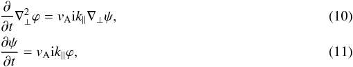 \arraycolsep0ptwith
 the Alfven velocity. These two equations are the standard linearized reduced-MHD equations
describing shear-Alfven waves with frequency:
the Alfven velocity. These two equations are the standard linearized reduced-MHD equations
describing shear-Alfven waves with frequency:
 (12)When the parallel electric
field is produced by a density fluctuation in Ohm’s law, we have
E∥ = − ik∥T0e(ne/n0).
Using the Poisson equation,
(12)When the parallel electric
field is produced by a density fluctuation in Ohm’s law, we have
E∥ = − ik∥T0e(ne/n0).
Using the Poisson equation,  , which also reveals the
vortical nature of the parallel electric field. The parameter
, which also reveals the
vortical nature of the parallel electric field. The parameter
 is the ion
gyroradius at the electron temperature. By including this parallel electric field in Ohm’s
law, an extension of the previous reduced-MHD system now takes the form
is the ion
gyroradius at the electron temperature. By including this parallel electric field in Ohm’s
law, an extension of the previous reduced-MHD system now takes the form 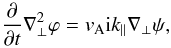 (13)
(13) (14)which describes the
dynamics of kinetic Alfven waves with frequency
(14)which describes the
dynamics of kinetic Alfven waves with frequency
 (15)It is worth noticing that
Eqs. (13), (14) can also be obtained directly from two-fluid MHD theory by retaining
the Hall and electron pressure effects in Ohm’s law (Bian
& Tsiklauri 2009). Using the above results, it is easily seen that, for
kinetic Alfven waves, the magnitude of the parallel electric field is related to
B⊥ by
(15)It is worth noticing that
Eqs. (13), (14) can also be obtained directly from two-fluid MHD theory by retaining
the Hall and electron pressure effects in Ohm’s law (Bian
& Tsiklauri 2009). Using the above results, it is easily seen that, for
kinetic Alfven waves, the magnitude of the parallel electric field is related to
B⊥ by
 (16)The above fluid
derivation of the Alfven wave frequency gives the same result as its kinetic counterpart,
however the latter, which is presented below, is more complete in the sense that it also
provides the imaginary part associated with Landau damping. The electron kinetic equation
can be solved for the perturbed distribution function f1, i.e.,
(16)The above fluid
derivation of the Alfven wave frequency gives the same result as its kinetic counterpart,
however the latter, which is presented below, is more complete in the sense that it also
provides the imaginary part associated with Landau damping. The electron kinetic equation
can be solved for the perturbed distribution function f1, i.e.,
 (17)Some notations are
introduced:
x = v∥/vte,
α = ω/k∥vte
and
(17)Some notations are
introduced:
x = v∥/vte,
α = ω/k∥vte
and  (18)with
Z0(α) the standard plasma dispersion
function. We also summarize some properties of the functions
Zn:
Z1 = 1 + αZ0,
Z2 = αZ1.
Moreover, in the limit α ≪ 1
(18)with
Z0(α) the standard plasma dispersion
function. We also summarize some properties of the functions
Zn:
Z1 = 1 + αZ0,
Z2 = αZ1.
Moreover, in the limit α ≪ 1
 (19)Using the above
properties, it follows that the density and current perturbations are related to the
parallel electric field through
(19)Using the above
properties, it follows that the density and current perturbations are related to the
parallel electric field through ![Mathematical equation: \begin{equation} \int f_{1}{\rm d}v_{\parallel}=\frac{2{\rm i}en_{0}}{m_{\rm e}k_{\parallel}v_{\rm te}^{2}}[1+\alpha Z_{0}(\alpha)]E_{\parallel}, \end{equation}](/articles/aa/full_html/2011/03/aa15385-10/aa15385-10-eq67.png) (20)for the density, and
(20)for the density, and
![Mathematical equation: \begin{equation} \int f_{1}v_{\parallel}{\rm d}v_{\parallel}=\frac{2{\rm i}en_{0}\omega}{m_{\rm e}k^{2}_{\parallel}v_{\rm te}^{2}}[1+\alpha Z_{0}(\alpha)]E_{\parallel}. \end{equation}](/articles/aa/full_html/2011/03/aa15385-10/aa15385-10-eq68.png) (21)As a result, the
relation between the parallel current and the parallel electric field is
(21)As a result, the
relation between the parallel current and the parallel electric field is
![Mathematical equation: \begin{equation} J_{\parallel}=\frac{-{\rm i} \omega}{4\pi k_{\parallel}^{2}\lambda_{\rm De}^{2}}[1+\alpha Z_{0}(\alpha)] E_{\parallel}. \end{equation}](/articles/aa/full_html/2011/03/aa15385-10/aa15385-10-eq69.png) (22)It is convenient to
define a collisionless plasma conductivity σ as
(22)It is convenient to
define a collisionless plasma conductivity σ as
 (23)Its imaginary part
results in the dispersion of the Alfven wave and its real part yields the collisionless
dissipation. In the limit
α ≡ ω/k∥vte ≪ 1,
the real part is
(23)Its imaginary part
results in the dispersion of the Alfven wave and its real part yields the collisionless
dissipation. In the limit
α ≡ ω/k∥vte ≪ 1,
the real part is  (24)This also gives the energy
per united time transferred to the electrons through the relation
(24)This also gives the energy
per united time transferred to the electrons through the relation
 (25)i.e.,
 (26)with
λDe the electron Debye length and
(26)with
λDe the electron Debye length and
 the
energy density of the parallel component of the electric field. It is, in fact, a standard
result that the asymptotic ωt ≫ 1 averaged power transferred to electrons,
the
energy density of the parallel component of the electric field. It is, in fact, a standard
result that the asymptotic ωt ≫ 1 averaged power transferred to electrons,
 , due to the presence of
an harmonic electric field fluctuation
E∥ = cos(k∥z − ωt),
is
, due to the presence of
an harmonic electric field fluctuation
E∥ = cos(k∥z − ωt),
is ![Mathematical equation: \begin{equation} Q=-\pi \frac{{\rm e}^{2}E^{2}_{\parallel}}{2m_{\rm e}k_{\parallel}}\left[v_{\parallel}\frac{\partial f_{0}}{\partial v_{\parallel}}\right]_{v_{\parallel}=\omega/k_{\parallel}}. \end{equation}](/articles/aa/full_html/2011/03/aa15385-10/aa15385-10-eq81.png) (27)It can be verified easily
from Eq. (1) and for a Maxwellian distribution that this last result is equivalent to
Eq. (26). Using the relation between E∥ and
B⊥, Q can finally be expressed in term of
the magnetic energy,
(27)It can be verified easily
from Eq. (1) and for a Maxwellian distribution that this last result is equivalent to
Eq. (26). Using the relation between E∥ and
B⊥, Q can finally be expressed in term of
the magnetic energy,  ,
,
 (28)The coefficient of
proportionality between Q and UB, which has the
dimension of the inverse of a time, is nothing else than the Landau damping rate.
(28)The coefficient of
proportionality between Q and UB, which has the
dimension of the inverse of a time, is nothing else than the Landau damping rate.
The Landau damping rate is now obtained directly from the complex dispersion relation. The
kinetic dispersion relation is obtained from: ![Mathematical equation: \hbox{$\nabla_{\perp}^{2}A_{\parallel}={\rm i}\omega/(k_{\parallel}^{2}\lambda_{\rm De}^{2}c)[1+\alpha Z_{0}(\alpha)]E_{\parallel}$}](/articles/aa/full_html/2011/03/aa15385-10/aa15385-10-eq87.png) ,
,
![Mathematical equation: \hbox{$\rho_{\rm s}^{2}\nabla_{\perp}^{2}\phi={\rm i}/k_{\parallel}[1+\alpha Z_{0}(\alpha)]E_{\parallel}$}](/articles/aa/full_html/2011/03/aa15385-10/aa15385-10-eq88.png) and
E∥ = −ik∥φ + iωA∥/c.
It is
and
E∥ = −ik∥φ + iωA∥/c.
It is ![Mathematical equation: \begin{equation} \rho_{\rm s}^{2}k^{2}_{\perp}+\left(1-\frac{\omega^{2}}{k_{\parallel}^{2}v_{\rm A}}\right)[1+\alpha Z_{0}(\alpha)]=0. \end{equation}](/articles/aa/full_html/2011/03/aa15385-10/aa15385-10-eq90.png) (29)This is the general
complex dispersion relation for the dispersive Alfven wave. In the limit
α ≪ 1, it reads as
(29)This is the general
complex dispersion relation for the dispersive Alfven wave. In the limit
α ≪ 1, it reads as ![Mathematical equation: \begin{equation} \omega^{2}=k^{2}_{\parallel}v_{\rm A}^{2}[1+k_{\perp}^{2}\rho^{2}_{\rm s}(1-{\rm i}\sqrt{\pi}\alpha)]. \end{equation}](/articles/aa/full_html/2011/03/aa15385-10/aa15385-10-eq92.png) (30)Its real part
corresponds to the frequency of the kinetic Alfven wave, which was also derived from fluid
theory above. Its imaginary part, which corresponds to the Landau damping rate (see also
Eq. (28)), reads as
(30)Its real part
corresponds to the frequency of the kinetic Alfven wave, which was also derived from fluid
theory above. Its imaginary part, which corresponds to the Landau damping rate (see also
Eq. (28)), reads as  (31)Most calculations above
were finalized in the limit α ≪ 1. In the opposite limit of
α ≫ 1, one obtains the frequency and damping rate of the inertial Alfven
wave, which has its parallel electric field balanced by the electron inertia in Ohm’s law.
For frequency
ω ~ k∥vA,
α ~ vA/vte.
It means that the kinetic Alfven wave regime corresponds to
vA/vte ≪ 1 and the inertial
Alfven wave regime corresponds to
vA/vte ≫ 1. In the following we
continue to focus on the warm plasma regime corresponding to
1 ≫ β ≫ me/mi,
where β is the pressure parameter. Landau damping of the inertial Alfven
wave and its effect on phase mixing can be treated similarly.
(31)Most calculations above
were finalized in the limit α ≪ 1. In the opposite limit of
α ≫ 1, one obtains the frequency and damping rate of the inertial Alfven
wave, which has its parallel electric field balanced by the electron inertia in Ohm’s law.
For frequency
ω ~ k∥vA,
α ~ vA/vte.
It means that the kinetic Alfven wave regime corresponds to
vA/vte ≪ 1 and the inertial
Alfven wave regime corresponds to
vA/vte ≫ 1. In the following we
continue to focus on the warm plasma regime corresponding to
1 ≫ β ≫ me/mi,
where β is the pressure parameter. Landau damping of the inertial Alfven
wave and its effect on phase mixing can be treated similarly.
3. Phase mixing
Phase mixing of a shear Alfven wave packet can be considered in the framework of an eikonal
description:  with
ω = ± k∥vA.
These are the characteristics of the wave-kinetic equation
with
ω = ± k∥vA.
These are the characteristics of the wave-kinetic equation
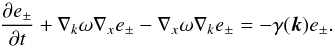 (34)In the latter equation
e ± are the amplitudes of the wave packets corresponding to
ω = ± k∥vA,
and γ(k) is a wave number dependent damping
rate. Following the trajectory of a wave packet in phase space
(x,k), its amplitude evolves
according to
(34)In the latter equation
e ± are the amplitudes of the wave packets corresponding to
ω = ± k∥vA,
and γ(k) is a wave number dependent damping
rate. Following the trajectory of a wave packet in phase space
(x,k), its amplitude evolves
according to  (35)This equation is
integrated to give
(35)This equation is
integrated to give  (36)The principle of
phase mixing is simple: for any damping rate γ that is an increasing
function of k, any mechanism producing an increase in k as
a function of time also results in a smaller damping time scale. This is precisely the
situation which occurs when the Alfven wave packet propagates along field lines with a
transverse variation of the Alfven speed: the wave packet is sheared. In this case, say
(36)The principle of
phase mixing is simple: for any damping rate γ that is an increasing
function of k, any mechanism producing an increase in k as
a function of time also results in a smaller damping time scale. This is precisely the
situation which occurs when the Alfven wave packet propagates along field lines with a
transverse variation of the Alfven speed: the wave packet is sheared. In this case, say
 ,
z is the unit vector in the parallel direction and
x the transverse coordinate, then
,
z is the unit vector in the parallel direction and
x the transverse coordinate, then
 (37)with by definition
 ,
L⊥ being the characteristic length of the transverse
inhomogeneity and
k∥ = k∥(t = 0).
This means that k⊥ increases linearly with time due to
differential advection of the wave packets along the field lines, i.e.,
,
L⊥ being the characteristic length of the transverse
inhomogeneity and
k∥ = k∥(t = 0).
This means that k⊥ increases linearly with time due to
differential advection of the wave packets along the field lines, i.e.,
 (38)where we have
taken k⊥(t = 0) = 0 without loss of
generality.
(38)where we have
taken k⊥(t = 0) = 0 without loss of
generality.
For resistive MHD, Ohm’s law reads as
E∥ = ηJ∥ and
the following results are well known. The damping rate is
 . This is the Fourier
transform of the operator responsible for magnetic diffusion in the induction equation.
Hence,
. This is the Fourier
transform of the operator responsible for magnetic diffusion in the induction equation.
Hence, ![Mathematical equation: \begin{equation} e_{\pm}(t)=e_{\pm}(0)\exp\left[-D_{m}k^{2}_{\parallel} \int(1+v_{\rm A}'^{2}t^{2}){\rm d}t\right], \end{equation}](/articles/aa/full_html/2011/03/aa15385-10/aa15385-10-eq122.png) (39)which in the limit
(39)which in the limit
 yields
  (40)Since,
z = vAt, we also have
(40)Since,
z = vAt, we also have
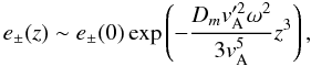 (41)for an Alfven wave
excited at z = 0 with frequency ω. In a collisionless
plasma, when the dissipation is provided by electron Landau damping, with damping rate
(41)for an Alfven wave
excited at z = 0 with frequency ω. In a collisionless
plasma, when the dissipation is provided by electron Landau damping, with damping rate
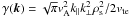 , the equivalent
expressions are
, the equivalent
expressions are 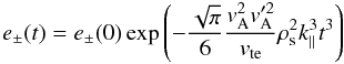 (42)and
 (43)for an Alfven wave
excited at z = 0 with frequency ω. The collisionless phase
mixing time scale is thus
(43)for an Alfven wave
excited at z = 0 with frequency ω. The collisionless phase
mixing time scale is thus 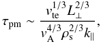 (44)and the phase mixing length
scale is
(44)and the phase mixing length
scale is 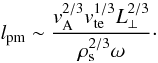 (45)The scaling of the
phase mixing length scale with the frequency ω in the spatial problem is
different from that of resistive MHD phase mixing since the collisionless conductivity
associated with electron Landau damping depends on ω, contrary to Spitzer
conductivity. However, the dependence with time or distance of the decay law, like
exp( − α1t3) or
exp( − α2z3) is similar to
resistive MHD phase mixing. The physical reason is obviously the common scaling of the
damping rate γ(k) with
k⊥ in the collisional and collisionless cases.
(45)The scaling of the
phase mixing length scale with the frequency ω in the spatial problem is
different from that of resistive MHD phase mixing since the collisionless conductivity
associated with electron Landau damping depends on ω, contrary to Spitzer
conductivity. However, the dependence with time or distance of the decay law, like
exp( − α1t3) or
exp( − α2z3) is similar to
resistive MHD phase mixing. The physical reason is obviously the common scaling of the
damping rate γ(k) with
k⊥ in the collisional and collisionless cases.
The effect of electron Landau damping on phase mixing was first considered by Voitenko & Goossens (2000a). They derived a
relation identical to Eq. (45) (see Eqs. (30) and (11) in Voitenko & Goossens 2000a). Moreover, results of the particles-in-cell
(PIC) simulations carried by Tsiklauri & Haruki
(2008) have produced
lpm ∝ ω − ζ
with ζ ≃ 1.10, for the dependence of the phase mixing length scale
lpm with frequency ω. They also report that
the parallel electric field associated with the Alfven wave is primarily balanced by the
electron pressure gradient in their simulations. They attribute the scaling of
lpm with ω to the effect of an anomalous
resistivity. Here, we emphasize that the PIC simulation results can be clearly interpreted
as the standard effect of electron Landau damping of the KAW by resonant interaction with
electrons since it gives
lpm ∝ ω − ζ
with ζ = 1. As a rule, the Landau damping rate is an increasing function of
frequency and, for kinetic Alfven waves, we have 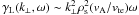 . In
contrast, the resistive damping rate is independent of frequency and is rewritten as
. In
contrast, the resistive damping rate is independent of frequency and is rewritten as
 , where
μe is the electron collisional frequency and
de = c/ωpe the
electron skin depth. Therefore, it is clear that Landau damping is the dominant damping
mechanism only for high-frequency Alfven waves, where
, where
μe is the electron collisional frequency and
de = c/ωpe the
electron skin depth. Therefore, it is clear that Landau damping is the dominant damping
mechanism only for high-frequency Alfven waves, where
 ,
,
 is the electron
pressure parameter. For typical coronal holes conditions,
vA/vte ~ 1/2 and
μe ~ 4 s-1, Landau damping dominates
resistivity for frequencies higher than ~1 s-1, and such
high-frequency Alfven waves can propagate a distance
is the electron
pressure parameter. For typical coronal holes conditions,
vA/vte ~ 1/2 and
μe ~ 4 s-1, Landau damping dominates
resistivity for frequencies higher than ~1 s-1, and such
high-frequency Alfven waves can propagate a distance 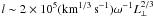 .
.
4. Parallel electric field generation
For an Alfven wave created by a source through perturbation of the background magnetic
field, a parallel electric field is produced, provided k⊥ is
finite, which is given by Eq. (16): 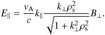 (46)It is this parallel
electric field that is responsible for the Landau damping of the wave (see above). For a
given k∥ and
δB⊥, this electric field is amplified
provided that the k⊥ associated with the wave field is also
amplified. The reason is that E∥ is a monotonic increasing
function of k⊥. However,
E∥(k⊥) also reaches a plateau
for k⊥ρs ~ 1, which is
the boundary between the MHD and the dispersive regime. Indeed,
(46)It is this parallel
electric field that is responsible for the Landau damping of the wave (see above). For a
given k∥ and
δB⊥, this electric field is amplified
provided that the k⊥ associated with the wave field is also
amplified. The reason is that E∥ is a monotonic increasing
function of k⊥. However,
E∥(k⊥) also reaches a plateau
for k⊥ρs ~ 1, which is
the boundary between the MHD and the dispersive regime. Indeed,
 (47)for
k⊥ρs ≪ 1 and
E∥ reaches its maximum, of the order of
(47)for
k⊥ρs ≪ 1 and
E∥ reaches its maximum, of the order of
 (48)when
k⊥ρs ~ 1 or larger.
Therefore, significant amplification of this parallel electric field can only occur in the
range of wave numbers where the wave is non-dispersive; i.e., it behaves as a shear-Alfven
wave with frequency
ω ≃ ± k∥vA.
(48)when
k⊥ρs ~ 1 or larger.
Therefore, significant amplification of this parallel electric field can only occur in the
range of wave numbers where the wave is non-dispersive; i.e., it behaves as a shear-Alfven
wave with frequency
ω ≃ ± k∥vA.
From the results of the previous section we obtain the dependence with time of the parallel
electric field strength during the phase mixing process:
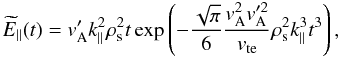 (49)where a normalized
electric field
(49)where a normalized
electric field 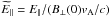 has been defined. The
variation with time
has been defined. The
variation with time  takes the form
β1texp( − α1t3),
with a growth phase followed by a decay phase typical of the alternating field aligned
current during phase mixing. Since
z = vAt, then
takes the form
β1texp( − α1t3),
with a growth phase followed by a decay phase typical of the alternating field aligned
current during phase mixing. Since
z = vAt, then
 (50)which has the form
β2zexp( − α2z3),
for an Alfven wave excited at z = 0 with frequency ω. The
above defined phase mixing time/length scales are precisely those scales associated with the
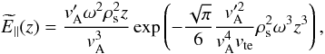
amplification of the parallel electric field; i.e., the time/length scales for the parallel
electric field to reach its maximum value given by
(50)which has the form
β2zexp( − α2z3),
for an Alfven wave excited at z = 0 with frequency ω. The
above defined phase mixing time/length scales are precisely those scales associated with the
amplification of the parallel electric field; i.e., the time/length scales for the parallel
electric field to reach its maximum value given by
 (51)with
ω ≃ k∥vA.
(51)with
ω ≃ k∥vA.
5. Conclusions
Previous PIC simulations of collisonless phase mixing of Alfven waves (Tsiklauri et al. 2005a,b; Tsiklauri & Haruki 2008) have identified its relation to the generation of a parallel electric field and acceleration of electrons. The importance of this parallel electric field has been first pointed out by Hasegawa and Chen in the context of resonant absorption. They also show that the dominant energy dissipation of the Alfven wave, in a collisionless low-β plasma, involves energy transfer to the electrons (Hasegawa & Chen 1976). The role of electron Landau damping in collisonless phase mixing has also been considered by Voitenko & Goossens (2000a,b)
Focusing on the kinetic regime of the dispersive Alfven wave, when vA/vte ≪ 1, we provided a detailed discussion of the role played by phase mixing in both parallel electric field amplification and enhanced electron Landau damping of the wave.
Qualitatively, the physics of collisionless phase mixing can be summarized as follows. A parallel electric field accompanies the propagation of Alfven waves with finite k⊥. The magnitude
of this electric field is an increasing function of k⊥ that
saturates in the dispersive range when
k⊥ρs ~ 1 or larger.
Therefore, any mechanism that produces an increase in k⊥ also
leads to the amplification of the parallel electric field associated with the Alfven wave.
Phase mixing is such a mechanism, independently of the energy dissipation channel. Phase
mixing is a special occurrence of energy-conserving cascade (Bian & Tsiklauri 2008). Such a cascade, predominantly involving
perpendicular wave numbers, can also be produced by non-linear interactions (i.e.
turbulence), leading to parallel electric field amplification (Bian & Kontar 2010; Bian et al.
2010). Existence of this parallel electric field and the dependence of its
magnitude with k⊥ yield a Landau damping rate, which scales
like  , just as
visco-resistive damping. This can be demonstrated very simply in the framework of
drift-kinetic theory. Therefore, in a collisionless plasma, phase mixing leads to enhanced
electron Landau damping of the Alfven wave in a manner that is very similar to the
well-studied case of enhanced visco-resistive damping. As a consequence, once the wave has
damped in a collisionless low-β plasma, its energy has been transferred to
the electrons. The time and length scales involved in the damping process were evaluated for
small amplitude perturbations. Moreover, we studied the evolution of the magnitude of the
parallel electric field in the course of its amplification and calculated its maximum value.
, just as
visco-resistive damping. This can be demonstrated very simply in the framework of
drift-kinetic theory. Therefore, in a collisionless plasma, phase mixing leads to enhanced
electron Landau damping of the Alfven wave in a manner that is very similar to the
well-studied case of enhanced visco-resistive damping. As a consequence, once the wave has
damped in a collisionless low-β plasma, its energy has been transferred to
the electrons. The time and length scales involved in the damping process were evaluated for
small amplitude perturbations. Moreover, we studied the evolution of the magnitude of the
parallel electric field in the course of its amplification and calculated its maximum value.
We argued that the scaling of the phase mixing length scale with frequency, lpm ∝ ω − ζ and ζ ≃ 1, reported by (Tsiklauri & Haruki 2008) has a simple interpretation in term of electron Landau damping. PIC simulations of collisionless phase mixing are valuable tools because they can provide direct information on the modification of the electron distribution function involved in the acceleration process, see (Tsiklauri et al. 2005a,b), a feature which the present kind of preliminary analysis is not capable of.
Acknowledgments
This work is supported by an STFC rolling grant (N.H.B., E.P.K.) and an STFC Advanced Fellowship (E.P.K.). Financial support by the Leverhulme Trust grant (F/00179/AY) and by the European Commission through the SOLAIRE Network (MTRN-CT-2006-035484) is gratefully acknowledged.
References
- Bian, N. H., & Kontar, E. P. 2010, Phys. Plasmas, 17, 062308 [NASA ADS] [CrossRef] [Google Scholar]
- Bian, N., & Tsiklauri, D. 2008, A&A, 489, 1291 [NASA ADS] [CrossRef] [EDP Sciences] [Google Scholar]
- Bian, N. H., & Tsiklauri, D. 2009, Phys. Plasmas, 16, 064503 [NASA ADS] [CrossRef] [Google Scholar]
- Bian, N. H., Kontar, E. P., & Brown, J. C. 2010, A&A, 519, A114 [NASA ADS] [CrossRef] [EDP Sciences] [Google Scholar]
- Botha, G. J. J., Arber, T. D., Nakariakov, V. M., & Keenan, F. P. 2000, A&A, 363, 1186 [NASA ADS] [Google Scholar]
- De Moortel, I., Hood, A. W., & Arber, T. D. 2000, A&A, 354, 334 [NASA ADS] [Google Scholar]
- Goertz, C. K., & Boswell, R. W. 1979, J. Geophys. Res., 84, 7239 [NASA ADS] [CrossRef] [Google Scholar]
- Hasegawa, A. 1976, J. Geophys. Res., 81, 5083 [NASA ADS] [CrossRef] [Google Scholar]
- Hasegawa, A. 1985, in Unstable Current Systems and Plasma Instabilities in Astrophysics, ed. M. R. Kundu, & G. D. Holman, IAU Symp., 107, 381 [Google Scholar]
- Hasegawa, A., & Chen, L. 1974, Phys. Rev. Lett., 32, 454 [NASA ADS] [CrossRef] [Google Scholar]
- Hasegawa, A., & Chen, L. 1976, Phys. Fluids, 19, 1924 [NASA ADS] [CrossRef] [Google Scholar]
- Hasegawa, A., & Mima, K. 1978, J. Geophys. Res., 83, 1117 [Google Scholar]
- Heyvaerts, J., & Priest, E. R. 1983, A&A, 117, 220 [NASA ADS] [Google Scholar]
- Hood, A. W., Brooks, S. J., & Wright, A. N. 2002, Roy. Soc. Lond. Proc. Ser. A, 458, 2307 [Google Scholar]
- Ionson, J. A. 1978, ApJ, 226, 650 [NASA ADS] [CrossRef] [Google Scholar]
- Nakariakov, V. M., Roberts, B., & Murawski, K. 1997, Sol. Phys., 175, 93 [NASA ADS] [CrossRef] [Google Scholar]
- Parker, E. N. 1991, ApJ, 376, 355 [NASA ADS] [CrossRef] [Google Scholar]
- Schekochihin, A. A., Cowley, S. C., Dorland, W., et al. 2009, ApJS, 182, 310 [NASA ADS] [CrossRef] [Google Scholar]
- Tsiklauri, D., & Haruki, T. 2008, Phys. Plasmas, 15, 112902 [NASA ADS] [CrossRef] [Google Scholar]
- Tsiklauri, D., Sakai, J., & Saito, S. 2005a, A&A, 435, 1105 [NASA ADS] [CrossRef] [EDP Sciences] [Google Scholar]
- Tsiklauri, D., Sakai, J., & Saito, S. 2005b, New J. Phys., 7, 79 [NASA ADS] [CrossRef] [Google Scholar]
- Voitenko, Y., & Goossens, M. 2000a, A&A, 357, 1086 [NASA ADS] [Google Scholar]
- Voitenko, Y., & Goossens, M. 2000b, A&A, 357, 1073 [NASA ADS] [Google Scholar]
Current usage metrics show cumulative count of Article Views (full-text article views including HTML views, PDF and ePub downloads, according to the available data) and Abstracts Views on Vision4Press platform.
Data correspond to usage on the plateform after 2015. The current usage metrics is available 48-96 hours after online publication and is updated daily on week days.
Initial download of the metrics may take a while.