| Issue |
A&A
Volume 527, March 2011
|
|
|---|---|---|
| Article Number | A68 | |
| Number of page(s) | 22 | |
| Section | Interstellar and circumstellar matter | |
| DOI | https://doi.org/10.1051/0004-6361/201015367 | |
| Published online | 26 January 2011 | |
Structure of evolved cluster-forming regions
1
Max-Planck-Institut für Radioastronomie,
Auf dem Hügel 69,
53121
Bonn,
Germany
e-mail: This email address is being protected from spambots. You need JavaScript enabled to view it.
2
I. Physikalisches Institut, Universität zu Köln,
Zülpicher Straße
77, 50937
Köln,
Germany
e-mail: This email address is being protected from spambots. You need JavaScript enabled to view it.
3
Centre for Star and Planet Formation, Natural History Museum of
Denmark, University of Copenhagen, Øster Voldgade 5-7, 1350
Copenhagen,
Denmark
Received:
9
July
2010
Accepted:
3
December
2010
Abstract
Context. An approach towards understanding the formation of massive stars and star clusters is to study the structure of their hot core phase, an evolutionary stage where dust has been heated, but molecules have not yet been destroyed by ultraviolet radiation. These hot molecular cores are very line-rich, but the interpretation of line surveys is also hampered by poor knowledge of the physical and chemical structure.
Aims. To constrain the radial structure of high-mass star-forming regions containing hot cores, we attempt to reproduce by radiative transfer modeling both the intensity and shape of a variety of molecular lines.
Methods. We observed 12 hot cores with the Atacama Pathfinder EXperiment (APEX) in lines of HCN, HCO+, CO, and their isotopologues, including high-J lines and vibrationally excited HCN. We investigate how well the sources can be modeled as centrally heated spheres with a power-law density gradient, making use of the radiative transfer code RATRAN and the radial profile of the submm continuum emission, taken from the APEX Telescope Large Area Survey of the GALaxy (ATLASGAL).
Results. Most of the observed lines have complicated shapes that incorporate self-absorption, asymmetries, and line wings. Vibrationally excited HCN is detected in all sources, and vibrationally excited H13CN in half of the sources. We are able to successfully model most features seen in the APEX data, such as the ratio of the isotopologue lines (very high optical depths), self-absorption (temperature gradient), blue asymmetries (moderate infall), vibrationally excited HCN (high inner temperatures), and H13CN (high HCN abundance under dense and hot conditions). Other features could not be reproduced, such as an occasional lack of self-absorption, the emission from high-J lines in the outer pixels of the CHAMP+ receiver (15′′−20′′ from the center), the outflow wings, and the red asymmetric profiles.
Conclusions. The amount of molecular gas, in particular of HCN, at very high temperatures is larger than previously thought. A complex interplay between infall and outflow motions is present. Our basic model assumptions of pure central heating and a power-law radial density distribution can serve as approximations for most sources, but are too simple to explain all observed lines. In particular, taking into account clumpiness, multiplicity of heating sources and a more complex velocity field seems to be necessary to more closely match model calculations to observations. This would require three-dimensional radiative transfer modeling of high-resolution interferometric data.
Key words: submillimeter: ISM / ISM: molecules / ISM: structure / ISM: clouds / stars: formation
© ESO, 2011
1. Introduction
Hot molecular cores are early stages of massive star formation, where stellar feedback is starting to affect the remnant core. The dense molecular gas out of which massive stars form is heated by their high luminosity, and shocks impinge on it, but it is not yet destroyed by ionization. While radiation from hypercompact Hii regions is observable in some cases, ionization is still kept too compact by the high densities caused, e.g., by ongoing accretion, to affect significant volumes (Walmsley 1995). Ice mantles around dust grains evaporate or are removed by shocks. Their complex chemistry and high temperatures make hot cores very line-rich and prominent targets for line surveys (e.g. Schilke et al. 2006; Belloche et al. 2007; Bergin et al. 2010). Owing to the large mass of warm dust, they are the brightest interstellar sources in the submm sky. Since high-mass stars quickly ionize their surroundings and drive out the gas, hot cores must be short-lived objects. They are indeed destroyed by the expanding ultracompact Hii regions ionized by their central star.
Despite their importance to both astrochemistry and massive star formation, little is known about the internal structure of hot cores and their envelopes (the distribution of density, temperature, molecular abundances, and velocity field). Reasons for this are difficulties in observations and in data analysis. These objects are compact ( ≈ 0.1 pc), rare (a few dozens are currently known in the Galaxy), and hence typically at large distances. The high dust column densities make them invisible in the near infrared and at shorter wavelengths. Single-dish radio and submm telescopes do not have high enough angular resolution to resolve the sources, and the still limited interferometer data available today are confusing and hard to interpret. Hot cores are found at the formation sites of clusters, so their structure is not simple and the interpretation of observations is not straightforward, but has to rely on radiative transfer modeling, i.e. a comparison between model and data.
Sources observed with the APEX telescope. Peak flux and full width at half-maximum are extracted from ATLASGAL (850 μm).
Several attempts have been made to model the structure of hot cores in spherical symmetry, often based on their spectral energy distribution (SED) (van der Tak 2002). For instance, Hatchell & van der Tak (2003) modeled the continuum and CS integrated line intensity, Osorio et al. (2009) reproduced the NH3 (4, 4) line in G31.41+0.31 (VLA, Cesaroni et al. 1998), or Nomura & Millar (2004) coupled physical and chemical models to predict abundances in Orion. However, no multi-line study trying to reproduce line shapes has yet been attempted. In this paper, we present APEX observations of many HCN, HCO+, and CO lines in 12 hot cores, as well as a comparison with models.
The models are spherically symmetric and have power-law density gradients. The temperature is determined self-consistently from central heating (Sect. 4.1). Continuum and line emission and absorption are computed using the code RATRAN (Hogerheijde & van der Tak 2000, Sect. 5.1). To avoid searching blindly in the large, multi-dimensional parameter space, we develop a method that approaches a possible good fit. From a grid of parameters, we select the models that fit the radial profile of the 850 μm continuum (Sect. 4), and identify suitable abundances (Sect. 5).
Frequency settings.
2. Observations and data reduction
APEX (Atacama Pathfinder Experiment)1 is a 12-m telescope located at 5100 m altitude in the northern Atacama desert in Chile (Güsten et al. 2006). This paper is based entirely on observations performed with this telescope. The sources observed are listed in Table 1. All data were taken in position switching mode, with the off positions 100′′ (wobbler for CHAMP+) or 400′′ (other settings) in azimuth from the source center. Beam sizes vary between 24′′ at 260 GHz, 18′′ at 345 GHz, 9′′ at 690 GHz, and 7′′ at 890 GHz. Pointing corrections were on the order of 5′′.
The first part of the data was taken in 2006 for eight sources. For the HCN 9–8 line, the FLASH receiver (Heyminck et al. 2006) and for the 4–3 lines, the APEX-2A receiver (Risacher et al. 2006) was used. Since these are double-sideband receivers, three settings with slightly different band center frequencies (spaced by 80 MHz) were taken to identify blending from the other sideband. In 2008, we observed lines from different isotopologues of HCN, HCO+, and CO with the APEX-1, APEX-2 (Vassilev et al. 2008), and CHAMP+ receivers (Kasemann et al. 2006; Güsten et al. 2008), all of which are single-sideband receivers. CHAMP+ allows simultaneous observations in the 690 GHz and the 850 GHz bands. Although it is a seven-pixel array receiver, we did not compile maps because the sources are very compact; we thus chose a higher signal-to-noise ratio (S/N) in the central pixel, and used the average of the outer pixels as an effective offset position (2.15 beam sizes, 15′′−20′′, from the center). The fast Fourier transform spectrometer (Klein et al. 2006) was used as the backend for all observations. Table 2 summarizes the frequency settings. In addition, CO 4–3 and 7–6 observations of nine sources performed by Friedrich Wyrowski, as well as observation of HCN lines from the line survey of G327.3-0.6 by Suzanne Bisschop were used to supplement our data set.
The data reduction involved the following steps. Using CLASS from the GILDAS software
package2, the individual scans were summed,
rejecting obviously bad ones. To convert from corrected antenna temperature
 to main-beam
brightness temperature Tmb, the intensity was multiplied by the
forward efficiency of 0.95 and divided by the main beam efficiency, which is 0.73 below
400 GHz. For the FLASH receiver, it is 0.6 below 600 GHz and 0.43 above (Güsten et al. 2006). For CHAMP+ in July 2008,
we adopted 0.28 below 750 GHz and 0.3 above. For the September 2008 data, we used 0.38 below
750 GHz and 0.35 above3
to main-beam
brightness temperature Tmb, the intensity was multiplied by the
forward efficiency of 0.95 and divided by the main beam efficiency, which is 0.73 below
400 GHz. For the FLASH receiver, it is 0.6 below 600 GHz and 0.43 above (Güsten et al. 2006). For CHAMP+ in July 2008,
we adopted 0.28 below 750 GHz and 0.3 above. For the September 2008 data, we used 0.38 below
750 GHz and 0.35 above3
A polynomial of order between 0 and 5 was fitted to the channels less affected by lines and used as a baseline that was subtracted from the spectra. The lines from HCN, HCO+, and CO were extracted, and, if necessary, another baseline subtraction was done. In some spectra, baseline ripples of period not much longer than the line width hampered this procedure. Finally, if lines were observed in different frequency settings, they were averaged to improve the S/N.
The intensity error can be estimated from varying intensities in these different settings. While it was usually within 30%, sometimes a factor of 2 or even 3 could be seen. Pointing was usually done on the source itself, but the drifting of the pointing and focus is a major problem for the high-frequency observations. The intensities of the HCN isotopologue lines are typically 30–50% larger in the APEX-2A data than in the APEX-2 data, sometimes twice as large. We chose to trust the newer APEX-2 observations, since for G327.3-0.6 they are consistent with Suzanne Bisschop’s data, taken with the same receiver. In addition, the APEX-2A receiver is known to have problems with varying sideband gain ratios affecting the calibration.
Radial 850 μm intensity profiles for all sources were extracted from ATLASGAL (APEX Telescope Large Area Survey of the Galaxy, Schuller et al. 2009), which uses LABOCA (Large APEX Bolometer Camera) on APEX (Siringo et al. 2009). The peak of the dust emission was taken as the center of the radial profiles. Regridding to 1′′ pixel size and radial averaging was done with MIRIAD4 (Sault et al. 1995).
Line ratios.
Integrated line intensities (in K km s-1).
Velocities of line peaks (in km s-1).
Line widths (full width at half-maximum in km s-1) derived from Gaussian fits to the lines.
3. Observational results
We present the results that we were able to directly derive from the observations. The spectra of those lines that were modeled (HCN, HCO+, and CO) are shown at the end of the paper. Additional information can best be obtained from the original data, which the interested reader can download5.
The most striking result is that we detect vibrationally excited HCN, whose level energies lie over 1000 K above the ground, in all sources, and even vibrationally excited H13CN in half of the sources (g327, i16, i17, b2n, b2m, g10). It is less clear whether we detect vibrationally excited HC15N, which is probably present in some sources. In contrast, there is not a single detection (with upper limits of around 0.1 K) of vibrationally excited HCO+, which has very similar level structure and line strengths.
Most lines have complicated shapes, with self-absorption often being present in the main isotopologues of HCN, HCO+, and CO. The notable two exceptions are i12 and w51d, whose HCN and HCO+ lines are singly peaked. The optical depth of all these lines must be very high, as seen from the other isotopologues. In the self-absorbed lines, the blue peak is always stronger in ngc, g10, g31, g34, w51e, and w51d, the red peak is always stronger in i17 and i12, and both asymmetries occur in g327, i16, b2n, and b2m. Line wings are also a prominent feature of these most optically thick lines. The lower level energies lie at 25 and 150 K for HCN and HCO+ 4–3 and 9–8, respectively, and at 33 and 117 K for CO 4–3 and 7–6, respectively.
To derive more quantitative information, we list the line parameters of selected lines: Table 3 compares the intensity ratios, Table 4 gives integrated line intensities, Table 5 presents the peak velocities, and Table 6 contains the line widths. However, we highlight that the optical depths are generally very high, so the lines are severely affected by gradients in excitation temperature, geometry, and velocity field, and can only be understood by means of radiative transfer modeling of the line shapes. For example, even the HC15N 4–3 line is optically thick towards the center of all models presented in Sect. 6.
4. Modeling procedure: continuum
We first attempt to reproduce the radial intensity profile from LABOCA. The temperature in our spherical model with density power law gradient is determined in an approximate way from central heating (Sect. 4.1). We set up a grid to cover the relevant ranges of parameters (Sect. 4.2), and select the models that are consistent with the continuum data (Sect. 4.3).
4.1. Temperature computation
We use an approximate method to determine the temperature in a spherical, centrally heated cloud with high column density. This method goes back to Larson (1969) and was also used in a similar way by Osorio et al. (1999).
In its inner parts, the dust is optically thick to its own radiation, which leads to diffusion of radiation. Both the dust temperature and density decrease outwards, both lowering the opacity because the decreasing temperature shifts the radiation field to longer wavelengths where the dust is less opaque. When the radiation is able to escape, a dust photosphere develops. This concept is similar to the effective radius of a star, where the whole luminosity would be emitted at one effective temperature. The photospheric radius separates the inner region, where diffusion determines the temperature gradient, from the outer region, where balance between heating and cooling determines the dust temperature.
The computation is done as follows. First, the Planck and Rosseland mean opacities are
computed from tabulated dust opacities by weighting with the Planck function, thus
converting frequency-dependent into temperature-dependent opacities. The photospheric
radius is given by  .
At larger radii, the balance between heating and cooling is
.
At larger radii, the balance between heating and cooling is
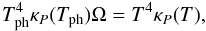 (1)where
 is the solid angle of the photosphere at radius r. This allows us to find
the radius for any temperature. At smaller radii, it is found by integrating the diffusion
equation that
is the solid angle of the photosphere at radius r. This allows us to find
the radius for any temperature. At smaller radii, it is found by integrating the diffusion
equation that  (2)The density
n is determined by the density power-law index p and
the assumption that the Rosseland optical depth at Tph from
the photospheric to the outer radius is 2/3.
(2)The density
n is determined by the density power-law index p and
the assumption that the Rosseland optical depth at Tph from
the photospheric to the outer radius is 2/3.
This method leads to a discontinuity at Rph, where the
temperature rises very slowly inwards and drops by a factor of
![Mathematical equation: \hbox{$\sqrt[4]{0.5}=0.84$}](/articles/aa/full_html/2011/03/aa15367-10/aa15367-10-eq53.png) outwards. To overcome this
artifact, we interpolate the temperature between
outwards. To overcome this
artifact, we interpolate the temperature between ![Mathematical equation: \hbox{$\sqrt[4]{0.5}T_{\rm ph}$}](/articles/aa/full_html/2011/03/aa15367-10/aa15367-10-eq54.png) and
and
![Mathematical equation: \hbox{$\sqrt[4]{2}T_{\rm ph}$}](/articles/aa/full_html/2011/03/aa15367-10/aa15367-10-eq55.png) as a power law.
as a power law.
In general, the temperature gradient is steeper in the inner parts of the cloud (where
the radii are smaller than Rph). One can see this by assuming
the behavior of the opacity to be proportional to
νβ, which renders the mean opacity
proportional to Tβ, and evaluating the
equations of heating/cooling balance and diffusion. The temperature in the outer parts
approaches  with the temperature power law-exponent
  .
In the inner part, the temperature also follows a power law, but with exponent
.
In the inner part, the temperature also follows a power law, but with exponent
 .
With β = 1 and p = 1.5, one has
qout = 0.4 and qin = 0.83. Using
tabulated opacities, the temperature gradients are similar to the these ones.
.
With β = 1 and p = 1.5, one has
qout = 0.4 and qin = 0.83. Using
tabulated opacities, the temperature gradients are similar to the these ones.
The following parameters can be set:
-
dust opacity (opac): a table with opacities at different wavelengths;
-
density power-law index (p): the density varies with radius r as r − p;
-
photospheric temperature (Tph): the effective temperature of the dust photosphere. It is a measure of the column density (the lower Tph, the higher the column density);
-
inner temperature (Tin): the temperature at the inner boundary;
-
outer temperature (Tout): the temperature at the outer boundary;
-
luminosity (L): the total energy output is not necessary for the computation, but the model size (radius) scales with
 ;
;
-
distance (dist): to compute the dust continuum flux received on Earth, the distance to the source is needed.
Average of the nmod selected models, with standard deviations of the parameters and derived properties (central column density of H2 in a pencil beam, total mass, mass above 100 K, inner, photospheric, and outer radii, density at the photospheric radius).
4.2. A grid of models
We hold the following parameters fixed: the distance at the value given in Table 1, the inner temperature at 1500 K (approximately the dust sublimation temperature), and the outer temperature at 20 K (temperature of the ambient cloud). An additional four parameters are instead varied:
-
Luminosity (L): we consider values a factor of 0.3–1 those in Table 1 (in steps of 0.1). The luminosity in the table is mostly derived from IRAS fluxes, but this more likely reflects the sum of all heating sources within the IRAS beam (there are often other Hii regions close to the hot core). Therefore, the true luminosity can be substantially lower than given in Table 1.
-
Photospheric temperature (Tph): to cover a wide range, we try values between 25 and 175 K, in steps of 2.5 K below 75 K and in steps of 5 K above.
-
Density gradient (p): the power-law exponent is varied between 1 and 2.25 in steps of 0.25.
-
Dust opacity (opac): we test four different opacities from Ossenkopf & Henning (1994), one with thin ice mantles and coagulation at a density of 106 cm-3 (thin,e6), the other three without grain mantles and either no coagulation (bare,no) or coagulation at a density of either 105 cm-3 (bare,e5) or 106 cm-3 (bare,e6)
4.3. Selection
The SED is contaminated by free-free radiation in the radio and other sources in the
far-IR, where the angular resolution is very low and the peak of the emission lies.
Therefore, we do not attempt to reproduce the SED, but take its integral as an upper limit
to the source luminosity and reproduce only the submm flux, where dust emission from the
hot core certainly dominates. For each of the 7680 models, a 345 GHz continuum map is then
computed by applying RATRAN. The map is convolved with the APEX beam and radial profiles
are extracted using MIRIAD. A model is assumed to successfully reproduce the LABOCA radial
profile if the following selection criteria are fulfilled: the peak intensity of the model
is between 0.75 and 1.25 times the observational value, its half-power width is smaller
than the observational value (since both other sources and observational problems such as
an incorrect focus or anomalous refraction tend to broaden the profile), and
 is below 1, with
 ,
where oi and
mi are the observed and modeled
intensities at i′′ from the center, respectively, and
Δoi is the rms deviation of the pixels
that were averaged to give oi.
,
where oi and
mi are the observed and modeled
intensities at i′′ from the center, respectively, and
Δoi is the rms deviation of the pixels
that were averaged to give oi.
The selected models (nmod out of 7680) span a cloud in
parameter space. For fixed opacity, the parameters are the density gradient
p, the luminosity L, and the photospheric temperature
Tph. We take the average (i.e., the center of the parameter
cloud) as a good representative of the selected models. Table 7 gives the averaged parameters, their standard deviations
 etc., and the most important properties of the models.
5. Modeling procedure: lines
We attempt to reproduce the lines from HCN, HCO+, and CO by developing detailed radiative-transfer models (Sect. 5.1). We explain which continuum-selected models we take as a physical structure to test several chemical structures (Sect. 5.2). We then attempt to improve the model fit to the emission lines by varying the abundances of the best-fit model (Sect. 5.3).
5.1. Line radiative transfer
To compute molecular lines, we use the Monte Carlo radiative-transfer code RATRAN developed by Hogerheijde & van der Tak (2000). We provide as input the physical structure from the continuum determination, with the gas temperature being equal to the dust temperature. This holds very well for the inner part with its high densities, and lies within the uncertainties for the outer part. The dust mass density is converted to H2 density by assuming a gas-to-dust mass ratio of 100 and that 74% of the gas mass is in the form of H2, 25% is helium, and 1% remaining elements. Additionally, the following information is needed:
-
Molecular data: energy levels, transition strengths, and collisional rate coefficients must be provided. For CO and HCO+ isotopologues, we use the entries from the LAMDA database (Schöier et al. 2005), cut above J = 20 (HCO+) and J = 17 (CO). For the vibrational bending mode (ν2) of HCN, each J has two vibrational levels (l-type doubling) about 1000 K above the ground state (Thorwirth et al. 2003; Fuchs et al. 2004). Collisional rates for them are unknown, and the computation for so many levels takes a very long time. Furthermore, the accuracy of the Monte Carlo calculations is insufficient for the tiny population difference of the two l-type levels, which are very close in energy. Therefore, we use only the first 15 ground-state levels for the Monte Carlo computation and extrapolate the other level populations in LTE relative to the corresponding ground-state J. This method gives very nearly the same results as the complete molecular data file (provided by van der Tak), since IR pumping of the ground-state levels operates mainly in regions where the levels are also collisionally excited. Collisional rates for J up to 8 and temperatures up to 99 K were provided by Faure and Wernli (2007, priv. comm.); the remainder, with a smooth transition, is from the LAMDA database (extrapolations from Green & Thaddeus 1974). Frequencies and Einstein A coefficients are from the Cologne Database for Molecular Spectroscopy (CDMS, Müller et al. 2001, 2005).
-
Velocity: the velocity field influences the line shapes. For a centrally heated source, the line profiles are found to be skewed towards the red by an outward motion and towards the blue by an inward motion, since the red side is more absorbed in the latter case. The asymmetry is stronger when the motion is faster (Evans 2003). We ignore the outflow wings, which come from non-spherical motions, by concentrating our attention on the line core. In spherical symmetry, outflows can not be accurately modeled. The velocity field that we use for ngc, b2m, g10, and g31 is 10% of free fall, i.e.
 ,
where Min is the mass inside the radius
r (starting with 50 M⊙ in the center,
but Min is quickly dominated by the surrounding
molecular gas). For g34 and w51e, it is 20% of free fall, while it is static (no
velocity field) for the remaining sources (i12, i16, g327, i17, b2n, w51d). Since
the modeled lines are not very sensitive to the exact radial behavior of the
velocity, we restricted ourselves to fractions of the free-fall velocity; the
adopted values are those that reproduce the data best.
,
where Min is the mass inside the radius
r (starting with 50 M⊙ in the center,
but Min is quickly dominated by the surrounding
molecular gas). For g34 and w51e, it is 20% of free fall, while it is static (no
velocity field) for the remaining sources (i12, i16, g327, i17, b2n, w51d). Since
the modeled lines are not very sensitive to the exact radial behavior of the
velocity, we restricted ourselves to fractions of the free-fall velocity; the
adopted values are those that reproduce the data best. -
Line width: internal motions broaden the lines. Interstellar line widths are generally dominated by turbulence or other macroscopic motions such as the relative motions of clumps rather than thermal motions. To reproduce the observed line widths, a 1/e half-width (0.6 of FWHM) of 3 km s-1 (5 km s-1FWHM) is adopted for all sources except g327 (2.5 km s-1; 4 km s-1FWHM) and b2n and b2m (7 km s-1; 12 km s-1FWHM). This reflects the different degrees of internal motions.
-
Abundance: the molecular abundances depend on the chemical evolution. Since modeling this is beyond the scope of the present analysis, we approximate variations with temperature as abundance jumps at certain temperatures. The HCN abundance rises with temperature (Rodgers & Charnley 2001; Garrod et al. 2008; Boonman et al. 2001), while the HCO+ abundance can be reduced at both low and high temperatures (Garrod et al. 2008). For CO, we assume a constant abundance of 10-4, while we derive the HCN and HCO+ abundances as described in Sect. 5.2.
-
Isotope ratios: the isotope ratios determine the relative abundances of the isotopologues, if isotope-sensitive chemistry can be neglected. Based on Wilson & Rood (1994), we use the following isotope ratios: for the Galactic center sources b2n and b2m 12C/13C = 20, 14N/15N = 600, 18O/16O = 250, 17O/16O = 800, for the nearby sources i17 and ngc 12C/13C = 70, 14N/15N = 450, 18O/16O = 550, 17O/16O = 1800, and for the rest 12C/13C = 50, 14N/15N = 400, 18O/16O = 300, 17O/16O = 1000. The variation with Galactocentric distance is thus approximate.
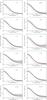 |
Fig. 1 Radial intensity profiles at 850 μm (LABOCA). The models from Table 8 are overlaid in red. The APEX beam is shown as a dashed Gaussian. The errorbars represent only the deviation from a circular shape, an additional error of 25% in the intensity would account for the calibration uncertainty. |
 |
Fig. 2 Lines towards G10.47+0.03. The model from Table 8 is overlaid in red. The lines are ordered on the same grid in all subsequent figures, apparent gaps indicate lines which were not observed. A green “B” stands for blending by a different line, an “O” means that the spectrum is likely to be affected by an outflow, which is not included in the model. |
5.2. Fitting strategy
The line computation can only be performed for a limited number of models, as it is highly demanding of computing power. On the basis of previous experience in the modeling, we devised the following general procedure.
We consider the opacity bare,e5, since that is a compromise between bare,no and bare,e6 and has a similar 850 μm opacity as thin,e6. In addition, the dust opacity being the same for every source facilitates a comparison. For this opacity, we consider three models, one close to the average, one with lower density gradient p, and one with higher p.
For each of the three models, we test freeze-out temperatures of 40 or 50 K (Garrod et al. 2008), depletion factors of 10, 100, or 1000, and chemical jump temperatures of 100, 150, or 230 K. Above the latter, HCO+ is reduced by a factor of 1000, while the HCN abundance is derived from its vibrational excitation. With seven freeze-out possibilities (either no depletion or two temperatures each with three depletion factors) and four high-temperature jump possibilities (no jump or three jump temperatures), there are 28 abundance structures of HCN and HCO+. The CO abundance is constant.
For an automatic adjustment of the abundance, an iterative procedure is employed to fit a line of low optical depth: the abundance is multiplied by the ratio of observed to modeled peak intensities; the computation stops when this ratio is close to 1 (within 25%) or when five cycles are reached. The line with the lowest optical depth, which is reliably detected, is used. For HCO+, we use the HC17O+ 3–2 line for b2n, b2m, g34, and w51e, HC18O+ 4–3 for i12, i16, ngc, and g31, and H13CO+ 4–3 for g327, i17, g10, and w51d. For HCN, we use the HC15N 4 − 3 line (3–2 in g34) to adjust the abundance below the chemical jump temperature. The abundance at high temperature is traced by HCN,v2 = 1, 3 − 2 for i12, ngc, g31, and w51d, 4–3 for g34 and w51e, and H13CN, v2 = 1, 8 − 7 for g327, i16, i17, b2n, b2m, and g10. The starting values are 10-10 for HCO+ and 10-9 for HCN between the jump temperatures.
5.3. The “final” model
As a figure of merit, we compute for each model and line
 ,
where oi and
mi are the observed and modeled
continuum-subtracted intensities, respectively, and nch the
number of channels between − 5 and +5 km s-1 from the source velocity. The
observational error is dominated by calibration uncertainties (assumed to be 30% of the
maximum intensity) rather than by thermal noise.
,
where oi and
mi are the observed and modeled
continuum-subtracted intensities, respectively, and nch the
number of channels between − 5 and +5 km s-1 from the source velocity. The
observational error is dominated by calibration uncertainties (assumed to be 30% of the
maximum intensity) rather than by thermal noise.
On the basis of a combination of the molecule-averaged χ2 and the normalized χ2 (the latter being the χ2 for the same peak intensities of model and data), we select the best-fit model from the different physical and chemical structures. By modifying the abundances of HCN and HCO+, we attempt to improve the fit. A constant CO abundance of 10-4 is assumed, since modifying this does not lead to significant improvements. This “final” model is an example of the best-fit solution that can be reached by this method, and is final in the sense that it probably cannot be improved significantly under our assumptions.
6. Modeling results
We present the results of the fitting strategy. For each source, the “final” model (parameters in Table 8) is compared to the line data, starting with the tighter fits (χ2 in Table 9). Figures 2 to 13 show the observed lines, superimposed on this model. The rotational lines of the HCN ground vibrational state are shown in the upper left, those of the vibrationally excited state (v2 = 1) in the lower left, HCO+ lines in the upper right, CO lines below that, and the lines from the outer pixels of CHAMP+ in the lower right. The vertical scale is the main beam brightness temperature in Kelvin. We note that some lines are affected by blending by neighboring lines, and in some sources broad CO and HCN lines blend vibrationally excited HCN and HC15N (at 265.8, 354.4, 345.8 and 691.5 GHz). This is indicated by a “B” in the spectrum. Some lines are so strongly blended that they cannot be used and are displayed for illustration purpose only. The strong lines from the main isotoplogues often have outflow wings, which are indicated by an “O” and not modeled. We note that this model is far from being unique, other selected physical structures with adapted abundances are also able to reproduce the data.
This model is compared to the continuum data in Fig. 1. The results of the continuum-only modeling are summarized in Table 7. Photospheric radii (for radiation of ≈ 40 − 90 K) are
around 0.1 pc, and the average gas density within it is usually several
106 cm-3 (a few times
105 M⊙ pc-3). The central optical
depth at 850 μm can be calculated from the column density
NH2 by multiplying it with 10-25 and
either 1.57 (bare,e6), 0.29 (bare,no), 0.83 (thin,e6), or 0.74 (bare,e5). It is usually
between 0.1 and 1. In addition, we find that Tph must increase
with L and p to fit the observations. In general, mass and
bolometric flux are proportional to L, the radii to
,
and the densities at these radii to  .
.
6.1. G10.47+0.03
This massive hot core has optically thick NH3(4, 4) satellites, and expansion motions can be traced by blue-shifted absorption against two hypercompact Hii regions (Cesaroni et al. 1994, 1998, 2010). The exceptionally high excitations and column densities of the core were also revealed by the HC3N study of Wyrowski et al. (1999). Olmi et al. (1996) detected different velocity gradients in CH3CN and 13CO, which are possibly indicative of rotation and outflow, respectively.
Figure 2 shows the observed lines and the best-fit model (Table 8). The line asymmetries are reproduced by a 10% free-fall contribution. Vibrationally excited H13CN is clearly detected, requiring a high abundance in the inner part (3 × 10⁻⁵ of H2). Owing to the large distance, the outer pixels are weak in this source. While the model fits quite well to the APEX data, our own SMA data reveal that this kind of model does not reproduce the innermost structure, since it is too strongly peaked (Rolffs et al., in prep.).
6.2. IRAS 16065-5158
Walsh et al. (1998) report the detection of an ultracompact Hii region associated with this source. The hot core was detected with the APEX telescope from a large sample of color-selected IRAS sources (Dedes et al. 2011).
Figure 3 shows the observed lines and the best-fit model (Table 8). The source is probably less concentrated than the model, since the 8–7 transitions of HCN and H13CN do not show self-absorption and the emission in the outer pixels is much stronger than modeled. We note that vibrationally excited H13CN and even HC15N (8–7 at 691.5 GHz) is detected here.
6.3. G327.3-0.6
G327.3-0.6 has a spectacular richness of lines with relatively narrow widths (Gibb et al. 2000; Schilke et al. 2006). The hot core is embedded in a larger structure, where different stages of star formation take place (Wyrowski et al. 2006; Minier et al. 2009).
Figure 4 shows the observed lines and the best-fit model (Table 8). The presence of both red and blue asymmetries indicates a complex velocity field. Vibrationally excited HCN, including its isotopologues, is very prominent in this source.
6.4. G34.26+0.15
This hot core lies off the bow of a cometary-shaped UCHii region (Watt & Mundy 1999). Therefore, it has been proposed to be externally heated by this Hii region (Mookerjea et al. 2007, and references therein). In this scenario, the emission from warm molecules arises in a relatively thin layer (PDR), while the inner cloud regions are cold.
However, we see no evidence for this in our data. Self-absorption and strong red asymmetries instead point to an infalling source with internal heating. We are perhaps able to probe larger scales, so external heating could be internal for our beam size. Figure 5 shows the observed lines and the best-fit model (Table 8).
6.5. G31.41+0.31
This hot core has a bipolar outflow (Olmi et al. 1996) and two continuum peaks (Cesaroni et al. 2010). A velocity gradient is interpreted as a massive toroidal disk by Beltrán et al. (2005) and an outflow by Araya et al. (2008).
Figure 6 shows the observed lines and the best-fit model (Table 8). No CHAMP+ observations were made for this source. With our data, we cannot distinguish between the proposed small-scale velocity fields.
6.6. IRAS 12326-6245
This hot core is associated with a massive molecular outflow and various infrared and radio sources (Henning et al. 2000).
Figure 7 shows the observed lines and the best-fit model (Table 8). The lack of self-absorption towards this source cannot be explained in the framework of our spherical models. To weaken self-absorption, the best-fit models have high freeze-out; but abundance variations at higher temperatures are not necessary. In addition, the outer pixels of CHAMP+ have much stronger line emission than modeled.
6.7. IRAS 17233-3606
IRAS 17233-3606 is a recently detected hot core (Leurini et al. 2008) with a close distance. It drives at least three outflows (Leurini et al. 2009), contains multiple radio sources (Zapata et al. 2008a), and displays a velocity gradient, which is interpreted by Beuther et al. (2009) as rotation, but could also be due to the superposition of outflows.
Figure 8 shows the observed lines and the best-fit model (Table 8). Broad line wings and blue asymmetries are probably caused by the outflows. In addition, the model has too much self-absorption and too little high-J line emission in the outer pixels. We see strong vibrationally excited H13CN.
6.8. NGC 6334-I
NGC 6334-I was extensively studied in line surveys (Thorwirth et al. 2007; Schilke et al. 2006). The SMA resolves the core into several mm peaks (Hunter et al. 2006), which show very different emission-line characteristics (Brogan et al. 2009). The large-scale environment was mapped by Walsh et al. (2010), and an outflow is also present (Beuther et al. 2008). This source was observed with Herschel/HIFI (Emprechtinger et al. 2010; Ceccarelli et al. 2010).
Figure 9 shows the observed lines and the best-fit model (Table 8). Owing, possibly, to the clumpiness, the high-J HCN lines are weaker and less self-absorbed than in the model.
6.9. W51e
W51e contains two hot cores, separated by 7′′ and associated with the UCHii regions e2 and e8 (Zhang et al. 1998). Both regions exhibit asymmetric line profiles, which were interpreted by Rudolph et al. (1990) as signatures of overall gravitational collapse. However, Ho & Young (1996) presented higher angular resolution observations and concluded that the collapse is localized to the two cores. Shi et al. (2010) shows that W51e2 has fragmented into additional pieces.
Figure 10 shows the observed lines and the best-fit model (Table 8). Both cores associated with e2 and e8 fall within our beam, which we had to ignore in the modeling. Our pointing was centered on the southern hot core (e1/e8). Infall is clearly seen by the strong blue asymmetries.
6.10. W51d
This hot core is located between the UCHii regions d1 and d2 (Zhang et al. 1998), and could host a rotating structure with outflow (Zapata et al. 2009). Infall motion is traced by SMA observations of CN absorption (Zapata et al. 2008b).
Figure 11 shows the observed lines and the best-fit model (Table 8). The lack of self-absorption cannot be explained by spherical symmetry. Line emission in the outer pixels of CHAMP+ is much stronger than modeled.
6.11. SgrB2(M)
SgrB2 Main contains a large number of UCHii regions (Gaume & Claussen 1990), and molecular gas of very high temperature is present (e.g. Wilson et al. 2006; Comito et al. 2003). The envelope was modeled by Lis & Goldsmith (1990).
Figure 12 shows the observed lines and the best-fit model (Table 8). Warm and dense clumps can be seen by the HCN and HCO+ emission in the outer pixels, which is not included in our model. Vibrationally excited H13CN is detected. Although the model incorporates infall, the asymmetry in the high-J lines points to an expanding velocity field in the inner part. We note that Herschel/HIFI data and a model that takes this into account are published in a separate paper (Rolffs et al. 2010).
6.12. SgrB2(N)
SgrB2 North is another very massive hot core 50′′ north of SgrB2(M), with a rich organic chemistry (e.g. Belloche et al. 2008). The hot and dense molecular gas is concentrated around the hypercompact Hii region K2 (Liu & Snyder 1999). de Vicente et al. (2000) showed with observations of vibrationally excited HC3N that hot cores are also present between M and N.
Figure 13 shows the observed lines and the best-fit model (Table 8). The strong and broad lines are not clearly reproduced by the model. Very broad absorption in the low-J lines are accompanied by redshifted absorption in the high-J lines, pointing to non-spherical infall. Vibrationally excited H13CN is present, and the outer pixels again show line emission (e.g. H13CN 8–7) that require high densities and temperatures at these locations, and hence clumpiness.
7. Discussion
The limitations of the data (too coarse angular resolution) and the radiative transfer modeling do not allow a reliable determination of the structure of the sources. Some observational features cannot be reproduced by any of the models, and the fits can be successfully performed by a variety of models. However, by systematically comparing models to the data, we can place some constraints on the source structure.
7.1. Heating engine
The high luminosities and submm fluxes imply that a massive (proto)star(s) is the heating engine. The lines from vibrationally excited HCN clearly show the high temperatures and the large heated mass. The self-absorption features prove the existence of a temperature gradient with lower temperatures closer to us. The observations are consistent with there being internal heating of the cores.
Although we model the sources with only one central star, we cannot exclude multiple heating sources. Multiplicity could indeed partly explain the deviations between model and data in many sources, and it is often observed by interferometers. This is unsurprising, because the sources are clusters in the making.
7.2. Density
Hot cores are basically heated density concentrations. For a power-law density distribution, an exponent of 1.5 seems consistent with the data, with a general tendency toward slightly larger values. The actual density depends on the dust opacity. For the opacity bare,e5 (Ossenkopf & Henning 1994) and a typical model, densities at the dust sublimation radius (a few hundred AU from the star) reach values as high as 109 cm-3 and fall off to 103 or 104 cm-3 at a radius of a pc, where the dust has cooled to the ambient temperature. Typical central column densities are 1025 cm-2.
Interferometer observations often reveal the presence of clumps, or in general a different small-scale density distribution than the strongly peaked one of our models. On larger scales, the rather strong lines in the outer pixels of CHAMP+ and the relatively little or no self-absorption in many sources are also indicative of clumpiness. The line emission in the CHAMP+ outer pixels clearly implies that there are higher densities at these locations. If that were the case for spherical (or cylindrical) symmetry, the continuum would be much higher than observed. A solution is the presence of high-density clumps, which provide the line emission but a moderate continuum due to beam dilution. The sources are likely to be embedded in a larger structure (see e.g. Myers 2009).
7.3. Velocity field
Infall motions are imprinted in the line shapes, as seen by blue asymmetries (lower velocities stronger). Freely contracting spheres (i.e., an inward velocity set by the mass inside) can be excluded, as in this case the lines would be far more asymmetric than observed. A tighter fit is obtained by reducing this free-fall speed to 10% in four sources (ngc, b2m, g10, g31) or 20% in two sources (w51e, g34). This corresponds to infall velocities of around 1 km s-1. We note that such a velocity field cannot be in a steady state, since the accretion rate decreases inwards. At the outer radius, these infall velocities correspond to cluster mass accretion rates of 10-3 to 10-1 solar masses per year. Dividing these rates by the source mass, each solar mass (representing a potential future star) would receive roughly 10-6 solar masses per year, and the timescale is thus 106 years. Since in the remaining six sources there are also symmetric or red asymmetric line profiles, a pure infall does not reproduce the lines well and we model them for now with zero velocity. The red asymmetric lines point to the presence of expansion motions, and we investigate this more complicated velocity field in a separate paper, based on Herschel/HIFI data (Rolffs et al. 2010).
In addition, we see high-velocity wings in many lines of CO, HCN, and HCO+, resulting from outflows (which would also destroy any spherical symmetry). The line width represents internal motions, which are several km s-1. The lowest amount of turbulence is found in g327, and the highest in the Galactic center sources b2n and b2m.
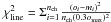
7.4. Molecular abundances
 |
Fig. 14 Mass fraction of hot gas vs. mass fraction of hot HCN in the best-fit models. Two groups of sources can be distinguished, one with detections of vibrationally excited H13CN, having an HCN abundance enhancement at high temperatures of around 100 and on average a higher fraction of hot gas, and one with an HCN abundance enhancement of around 25, coming from freeze-out of HCN at low temperatures. |
For the densities corresponding to the dust opacity bare,e5, we find typical abundances relative to H2 of 10-7 (HCN), 10-8 (HCO+), and 10-4 (CO). While we allow the CO abundance to be exactly 10-4 everywhere, the mentioned abundances of HCN and HCO+ are only an order of magnitude between 50 and 100 K. On the basis of Garrod et al. (2008), we allow a reduced abundance of these molecules below 40 or 50 K (due to molecular depletion), and this is actually needed to reproduce the observed self-absorptions. An evaporation temperature of 100 K, together with water, would not match most of the observed lines.
In sources where vibrationally excited H13CN is detected, HCN must be very abundant at high temperatures (10-6 to several 10-5), which is consistent with predictions from chemical models (Rodgers & Charnley 2001) and also needed by Boonman et al. (2001). However, the astrochemical reason for this very high abundance remains unclear. Figure 14 shows the abundance enhancement in the models, allowing us to identify the two groups with and without vibrationally excited H13CN. The former group has on average not only a larger fraction of hot gas, but also a higher HCN abundance in this gas.
In contrast, no vibrationally excited HCO+ is detected. Since it has a very similar level structure and line strengths as HCN, this non-detection means that it must be much less abundant than HCN at high temperatures. Relative to the HCN (and H13CN) abundances and intensities of the vibrational lines, the HCO+ abundance cannot be higher than about 10-8 above 100 K. We allow a reduced abundance of HCO+ at high temperatures (van der Tak & van Dishoeck 2000), but our data are of insufficient quality to constrain this.
7.5. Limitations of our modeling approach
We first note that we are limited to spherical symmetry. However, two- or three-dimensional modeling would not be reliably constrained by our data; the lines need to be spatially well resolved to achieve this. Consequently, we chose to consider only centrally heated models. The density was assumed to follow a power law. While this strong central condensation is consistent with the framework of central heating, a more realistic picture of a forming star cluster would include multiple heating sources and likely a central flattening of the density. These possibilities are not covered by our modeling, nor is a clumpy, geometrically flattened or filamentary structure. In addition, outflows cannot be considered in spherically symmetric models.
The grid that we use for the continuum-relevant parameters is complete enough, but the selection of models relies on the LABOCA data, which do not have sufficient angular resolution. Owing to limited computational power, we could not test all selected models, and only a few chemical structures, thus we were unable to find the optimal global combination of the parameters. In addition, the chemical structures are crude approximations of the abundance variations, and are not computed from chemical models. The dust opacity is assumed to be constant throughout the source, although it is likely to vary (e.g. due to evaporation of ice mantles).
8. Conclusions
We have observed a sample of 12 hot cores in lines of HCN, HCO+, and CO with the APEX telescope. With the aim of reproducing the line shapes, we tested spherical models with density power-law gradients and central heating. Our results can be summarized as follows:
-
1.
Vibrational excitation: vibrationally excited HCN (1000 K above ground) is very prominent in our sources, and even vibrationally excited H13CN is clearly detected in half of them (g327, i16, i17, b2n, b2m, g10). This result is surprising because it means that vibrationally excited HCN is optically thick and that there is much more hot gas than previously thought. The lines are still visible at 800 GHz, meaning that dust does not obscure the hot gas at these frequencies. They can be well modeled; to reproduce vibrationally excited H13CN, an enhanced HCN abundance at high temperatures is necessary. On the other hand, no vibrationally excited HCO+ is detected. Given its very similar molecular structure, this means it is much less abundant than HCN under hot, dense conditions.
-
2.
Self-absorption: in most sources, the main transitions are heavily self-absorbed. This finding, together with the corresponding lines from more rare isotopologues, is qualitatively reproduced by our models. It is caused by very high optical depths and the temperature gradient, and depends also on the abundance structure (e.g. freeze-out). However, well-peaked, but highly optically thick lines, similar to those found in w51d and i12, cannot be modeled in our framework, and must be produced by geometry effects.
-
3.
Outer pixels: the high-frequency CHAMP+ receiver on APEX has seven pixels. We were mainly interested in the central pixel, but also modeled the average of the other pixels, which are about two beam sizes (15′′ − 20′′) from the center. The modeling always leads to much lower intensities in the outer pixels than observed. We conclude that the warm, dense gas is not as highly concentrated as predicted by our models, which have steep radial gradients in temperature and density. Clumpiness and multiple heating sources are present instead, as expected for a cluster environment.
-
4.
Velocity field: information about the velocity field is encoded in the line shapes, in particular their asymmetries. The blue side (lower velocities) is in most cases stronger than the red side, which we model as an inward velocity. The free-fall speed, which would be unhampered contraction, must be reduced to 10 or 20% to reproduce the line shapes. This means that there is infall, but also mechanisms to slow it down. However, we have modeled half of our sources as static, since the velocity field is often more complicated, shown by outflow wings in CO, symmetric lines, and red asymmetries. This means that expansion motions are also present in some sources, e.g. b2m and g327, caused by the onset of feedback from massive stars (see the paper on Herschel/HIFI data of b2m, Rolffs et al. 2010).
-
5.
Basic assumptions: for the radiative transfer modeling, we are limited to a very simplified source structure. In particular, we assume spherical symmetry with a radial power-law gradient in density and pure central heating, which provides a rough approximation of the temperature. Molecular abundances are not computed from chemical models, but variations are approximated as jumps at certain temperatures. While these crude simplifications are able to explain many observational features, the assumptions are too simple to reproduce everything. Three-dimensional radiative transfer, coupled to physical and chemical models and based on high-resolution interferometric data, is needed to reliably determine the structure of hot cores.
This publication is based on data acquired with the Atacama Pathfinder EXperiment (APEX). APEX is a collaboration between the Max-Planck-Institut für Radioastronomie, the European Southern Observatory, and the Onsala Space Observatory.
Acknowledgments
We thank Floris van der Tak for the molecular data of vibrationally excited HCN and for the support with RATRAN. R. Rolffs acknowledges support by the International Max Planck Research School for Astronomy and Astrophysics. We thank Claudia Comito for help in the acquisition of the first part of the data.
References
- Araya, E., Hofner, P., Kurtz, S., Olmi, L., & Linz, H. 2008, ApJ, 675, 420 [NASA ADS] [CrossRef] [Google Scholar]
- Belloche, A., Comito, C., Hieret, C., et al. 2007, in Molecules in Space and Laboratory, 10 [Google Scholar]
- Belloche, A., Menten, K. M., Comito, C., et al. 2008, A&A, 482, 179 [NASA ADS] [CrossRef] [EDP Sciences] [Google Scholar]
- Beltrán, M. T., Cesaroni, R., Neri, R., et al. 2005, A&A, 435, 901 [NASA ADS] [CrossRef] [EDP Sciences] [Google Scholar]
- Bergin, E. A., Phillips, T. G., Comito, C., et al. 2010, A&A, 521, L20 [NASA ADS] [CrossRef] [EDP Sciences] [Google Scholar]
- Beuther, H., Walsh, A. J., Thorwirth, S., et al. 2008, A&A, 481, 169 [NASA ADS] [CrossRef] [EDP Sciences] [Google Scholar]
- Beuther, H., Walsh, A. J., & Longmore, S. N. 2009, ApJS, 184, 366 [NASA ADS] [CrossRef] [Google Scholar]
- Boonman, A. M. S., Stark, R., van der Tak, F. F. S., et al. 2001, ApJ, 553, L63 [NASA ADS] [CrossRef] [Google Scholar]
- Brogan, C. L., Hunter, T. R., Indebetouw, R., et al. 2009, in BAAS, 41, 499 [Google Scholar]
- Ceccarelli, C., Bacmann, A., Boogert, A., et al. 2010, A&A, 521, L22 [NASA ADS] [CrossRef] [EDP Sciences] [Google Scholar]
- Cesaroni, R., Churchwell, E., Hofner, P., Walmsley, C. M., & Kurtz, S. 1994, A&A, 288, 903 [NASA ADS] [Google Scholar]
- Cesaroni, R., Hofner, P., Walmsley, C. M., & Churchwell, E. 1998, A&A, 331, 709 [NASA ADS] [Google Scholar]
- Cesaroni, R., Hofner, P., Araya, E., & Kurtz, S. 2010, A&A, 509, A50 [NASA ADS] [CrossRef] [EDP Sciences] [Google Scholar]
- Churchwell, E., Walmsley, C. M., & Cesaroni, R. 1990, A&AS, 83, 119 [Google Scholar]
- Comito, C., Schilke, P., Gerin, M., et al. 2003, A&A, 402, 635 [NASA ADS] [CrossRef] [EDP Sciences] [Google Scholar]
- de Vicente, P., Martín-Pintado, J., Neri, R., & Colom, P. 2000, A&A, 361, 1058 [NASA ADS] [Google Scholar]
- Dedes, C., Leurini, S., Wyrowski, F., et al. 2011, A&A, 526, A59 [NASA ADS] [CrossRef] [EDP Sciences] [Google Scholar]
- Emprechtinger, M., Lis, D. C., Bell, T., et al. 2010, A&A, 521, L28 [NASA ADS] [CrossRef] [EDP Sciences] [Google Scholar]
- Evans, II, N. 2003, in SFChem 2002: Chemistry as a Diagnostic of Star Formation, ed. C. L. Curry, & M. Fich, 157 [Google Scholar]
- Faúndez, S., Bronfman, L., Garay, G., et al. 2004, A&A, 426, 97 [NASA ADS] [CrossRef] [EDP Sciences] [Google Scholar]
- Fuchs, U., Bruenken, S., Fuchs, G. W., et al. 2004, Z. Naturforsch. A, 59, 861 [NASA ADS] [Google Scholar]
- Garrod, R. T., Weaver, S. L. W., & Herbst, E. 2008, ApJ, 682, 283 [NASA ADS] [CrossRef] [Google Scholar]
- Gaume, R. A., & Claussen, M. J. 1990, ApJ, 351, 538 [NASA ADS] [CrossRef] [Google Scholar]
- Gibb, E., Nummelin, A., Irvine, W. M., Whittet, D. C. B., & Bergman, P. 2000, ApJ, 545, 309 [NASA ADS] [CrossRef] [PubMed] [Google Scholar]
- Goldsmith, P. F., Lis, D. C., Lester, D. F., & Harvey, P. M. 1992, ApJ, 389, 338 [NASA ADS] [CrossRef] [Google Scholar]
- Green, S., & Thaddeus, P. 1974, ApJ, 191, 653 [NASA ADS] [CrossRef] [Google Scholar]
- Güsten, R., Nyman, L. Å., Schilke, P., et al. 2006, A&A, 454, L13 [NASA ADS] [CrossRef] [EDP Sciences] [Google Scholar]
- Güsten, R., Baryshev, A., Bell, A., et al. 2008, in Presented at the Society of Photo-Optical Instrumentation Engineers (SPIE) Conference, Society of Photo-Optical Instrumentation Engineers (SPIE) Conf. Ser., 7020 [Google Scholar]
- Hatchell, J., & van der Tak, F. F. S. 2003, A&A, 409, 589 [NASA ADS] [CrossRef] [EDP Sciences] [Google Scholar]
- Henning, T., Lapinov, A., Schreyer, K., Stecklum, B., & Zinchenko, I. 2000, A&A, 364, 613 [NASA ADS] [Google Scholar]
- Heyminck, S., Kasemann, C., Güsten, R., de Lange, G., & Graf, U. U. 2006, A&A, 454, L21 [NASA ADS] [CrossRef] [EDP Sciences] [Google Scholar]
- Ho, P. T. P., & Young, L. M. 1996, ApJ, 472, 742 [NASA ADS] [CrossRef] [Google Scholar]
- Hogerheijde, M. R., & van der Tak, F. F. S. 2000, A&A, 362, 697 [NASA ADS] [Google Scholar]
- Hunter, T. R., Brogan, C. L., Megeath, S. T., et al. 2006, ApJ, 649, 888 [NASA ADS] [CrossRef] [Google Scholar]
- Kasemann, C., Güsten, R., Heyminck, S., et al. 2006, in Presented at the Society of Photo-Optical Instrumentation Engineers (SPIE) Conference, Society of Photo-Optical Instrumentation Engineers (SPIE) Conf. Ser., 6275 [Google Scholar]
- Klein, B., Philipp, S. D., Krämer, I., et al. 2006, A&A, 454, L29 [NASA ADS] [CrossRef] [EDP Sciences] [Google Scholar]
- Larson, R. B. 1969, MNRAS, 145, 297 [NASA ADS] [Google Scholar]
- Leurini, S., Hieret, C., Thorwirth, S., et al. 2008, A&A, 485, 167 [NASA ADS] [CrossRef] [EDP Sciences] [Google Scholar]
- Leurini, S., Codella, C., Zapata, L. A., et al. 2009, A&A, 507, 1443 [NASA ADS] [CrossRef] [EDP Sciences] [Google Scholar]
- Lis, D. C., & Goldsmith, P. F. 1990, ApJ, 356, 195 [NASA ADS] [CrossRef] [Google Scholar]
- Liu, S.-Y., & Snyder, L. E. 1999, ApJ, 523, 683 [NASA ADS] [CrossRef] [Google Scholar]
- MacLeod, G. C., Scalise, E. J., Saedt, S., Galt, J. A., & Gaylard, M. J. 1998, AJ, 116, 1897 [NASA ADS] [CrossRef] [Google Scholar]
- Minier, V., André, P., Bergman, P., et al. 2009, A&A, 501, L1 [NASA ADS] [CrossRef] [EDP Sciences] [Google Scholar]
- Mookerjea, B., Casper, E., Mundy, L. G., & Looney, L. W. 2007, ApJ, 659, 447 [NASA ADS] [CrossRef] [Google Scholar]
- Müller, H. S. P., Thorwirth, S., Roth, D. A., & Winnewisser, G. 2001, A&A, 370, L49 [NASA ADS] [CrossRef] [EDP Sciences] [Google Scholar]
- Müller, H. S. P., Schlöder, F., Stutzki, J., & Winnewisser, G. 2005, J. Mol. Struct., 742, 215 [NASA ADS] [CrossRef] [Google Scholar]
- Myers, P. C. 2009, ApJ, 700, 1609 [NASA ADS] [CrossRef] [EDP Sciences] [Google Scholar]
- Neckel, T. 1978, A&A, 69, 51 [NASA ADS] [Google Scholar]
- Nomura, H., & Millar, T. J. 2004, A&A, 414, 409 [NASA ADS] [CrossRef] [EDP Sciences] [MathSciNet] [Google Scholar]
- Olmi, L., Cesaroni, R., Neri, R., & Walmsley, C. M. 1996, A&A, 315, 565 [NASA ADS] [Google Scholar]
- Osorio, M., Lizano, S., & D’Alessio, P. 1999, ApJ, 525, 808 [NASA ADS] [CrossRef] [Google Scholar]
- Osorio, M., Anglada, G., Lizano, S., & D’Alessio, P. 2009, ApJ, 694, 29 [NASA ADS] [CrossRef] [Google Scholar]
- Ossenkopf, V., & Henning, T. 1994, A&A, 291, 943 [NASA ADS] [Google Scholar]
- Osterloh, M., Henning, T., & Launhardt, R. 1997, ApJS, 110, 71 [NASA ADS] [CrossRef] [Google Scholar]
- Pandian, J. D., Momjian, E., & Goldsmith, P. F. 2008, A&A, 486, 191 [NASA ADS] [CrossRef] [EDP Sciences] [Google Scholar]
- Reid, M. J., Menten, K. M., Zheng, X. W., Brunthaler, A., & Xu, Y. 2009, ApJ, 705, 1548 [NASA ADS] [CrossRef] [Google Scholar]
- Risacher, C., Vassilev, V., Monje, R., et al. 2006, A&A, 454, L17 [NASA ADS] [CrossRef] [EDP Sciences] [Google Scholar]
- Rodgers, S. D., & Charnley, S. B. 2001, ApJ, 546, 324 [Google Scholar]
- Rolffs, R., Schilke, P., Comito, C., et al. 2010, A&A, 521, L46 [NASA ADS] [CrossRef] [EDP Sciences] [Google Scholar]
- Rudolph, A., Welch, W. J., Palmer, P., & Dubrulle, B. 1990, ApJ, 363, 528 [NASA ADS] [CrossRef] [Google Scholar]
- Sandell, G. 2000, A&A, 358, 242 [NASA ADS] [Google Scholar]
- Sato, M., Reid, M. J., Brunthaler, A., & Menten, K. M. 2010, ApJ, 720, 1055 [NASA ADS] [CrossRef] [Google Scholar]
- Sault, R. J., Teuben, P. J., & Wright, M. C. H. 1995, in Astronomical Data Analysis Software and Systems IV, ed. R. A. Shaw, H. E. Payne, & J. J. E. Hayes, ASP Conf. Ser., 77, 433 [Google Scholar]
- Schilke, P., Comito, C., Thorwirth, S., et al. 2006, A&A, 454, L41 [NASA ADS] [CrossRef] [EDP Sciences] [Google Scholar]
- Schöier, F. L., van der Tak, F. F. S., van Dishoeck, E. F., & Black, J. H. 2005, A&A, 432, 369 [NASA ADS] [CrossRef] [EDP Sciences] [Google Scholar]
- Schuller, F., Menten, K. M., Contreras, Y., et al. 2009, A&A, 504, 415 [NASA ADS] [CrossRef] [EDP Sciences] [Google Scholar]
- Shi, H., Zhao, J., & Han, J. L. 2010, ApJ, 710, 843 [NASA ADS] [CrossRef] [Google Scholar]
- Simpson, J. P., & Rubin, R. H. 1990, ApJ, 354, 165 [NASA ADS] [CrossRef] [Google Scholar]
- Siringo, G., Kreysa, E., Kovács, A., et al. 2009, A&A, 497, 945 [NASA ADS] [CrossRef] [EDP Sciences] [Google Scholar]
- Thorwirth, S., Müller, H. S. P., Lewen, F., et al. 2003, ApJ, 585, L163 [NASA ADS] [CrossRef] [Google Scholar]
- Thorwirth, S., Walsh, A. J., Wyrowski, F., et al. 2007, in Molecules in Space and Laboratory, ed. J. L. Lemaire, & F. Combes, 39 [Google Scholar]
- van der Tak, F. F. S. 2002, in Hot Star Workshop III: The Earliest Phases of Massive Star Birth, ed. P. Crowther, ASP Conf. Ser., 267, 33 [NASA ADS] [Google Scholar]
- van der Tak, F. F. S., & van Dishoeck, E. F. 2000, A&A, 358, L79 [NASA ADS] [Google Scholar]
- Vassilev, V., Meledin, D., Lapkin, I., et al. 2008, A&A, 490, 1157 [NASA ADS] [CrossRef] [EDP Sciences] [Google Scholar]
- Walmsley, M. 1995, in Rev. Mex. Astron. Astrofis., 27, ed. S. Lizano, & J. M. Torrelles, Rev. Mex. Astron. Astrofis. Conf. Ser., 1, 137 [Google Scholar]
- Walsh, A. J., Burton, M. G., Hyland, A. R., & Robinson, G. 1998, MNRAS, 301, 640 [NASA ADS] [CrossRef] [Google Scholar]
- Walsh, A. J., Thorwirth, S., Beuther, H., & Burton, M. G. 2010, MNRAS, 404, 1396 [NASA ADS] [Google Scholar]
- Watt, S., & Mundy, L. G. 1999, ApJS, 125, 143 [NASA ADS] [CrossRef] [Google Scholar]
- Wilson, T. L., & Rood, R. 1994, ARA&A, 32, 191 [NASA ADS] [CrossRef] [Google Scholar]
- Wilson, T. L., Henkel, C., & Hüttemeister, S. 2006, A&A, 460, 533 [NASA ADS] [CrossRef] [EDP Sciences] [Google Scholar]
- Wyrowski, F., Schilke, P., & Walmsley, C. M. 1999, A&A, 341, 882 [NASA ADS] [Google Scholar]
- Wyrowski, F., Menten, K. M., Schilke, P., et al. 2006, A&A, 454, L91 [NASA ADS] [CrossRef] [EDP Sciences] [Google Scholar]
- Zapata, L. A., Leurini, S., Menten, K. M., et al. 2008a, AJ, 136, 1455 [NASA ADS] [CrossRef] [Google Scholar]
- Zapata, L. A., Palau, A., Ho, P. T. P., et al. 2008b, A&A, 479, L25 [NASA ADS] [CrossRef] [EDP Sciences] [Google Scholar]
- Zapata, L. A., Ho, P. T. P., Schilke, P., et al. 2009, ApJ, 698, 1422 [NASA ADS] [CrossRef] [Google Scholar]
- Zhang, Q., Ho, P. T. P., & Ohashi, N. 1998, ApJ, 494, 636 [NASA ADS] [CrossRef] [Google Scholar]
All Tables
Sources observed with the APEX telescope. Peak flux and full width at half-maximum are extracted from ATLASGAL (850 μm).
Line widths (full width at half-maximum in km s-1) derived from Gaussian fits to the lines.
Average of the nmod selected models, with standard deviations of the parameters and derived properties (central column density of H2 in a pencil beam, total mass, mass above 100 K, inner, photospheric, and outer radii, density at the photospheric radius).
All Figures
|
Fig. 1 Radial intensity profiles at 850 μm (LABOCA). The models from Table 8 are overlaid in red. The APEX beam is shown as a dashed Gaussian. The errorbars represent only the deviation from a circular shape, an additional error of 25% in the intensity would account for the calibration uncertainty. |
| In the text | |
|
Fig. 2 Lines towards G10.47+0.03. The model from Table 8 is overlaid in red. The lines are ordered on the same grid in all subsequent figures, apparent gaps indicate lines which were not observed. A green “B” stands for blending by a different line, an “O” means that the spectrum is likely to be affected by an outflow, which is not included in the model. |
| In the text | |
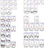 |
Fig. 3 Lines towards IRAS 16065-5158. The model from Table 8 is overlaid in red. |
| In the text | |
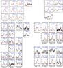 |
Fig. 4 Lines towards G327.3-0.6. The model from Table 8 is overlaid in red. |
| In the text | |
 |
Fig. 5 Lines towards G34.26+0.15. The model from Table 8 is overlaid in red. |
| In the text | |
 |
Fig. 6 Lines towards G31.41+0.31. The model from Table 8 is overlaid in red. |
| In the text | |
 |
Fig. 7 Lines towards IRAS 12326-6245. The model from Table 8 is overlaid in red. |
| In the text | |
 |
Fig. 8 Lines towards IRAS 17233-3606. The model from Table 8 is overlaid in red. |
| In the text | |
 |
Fig. 9 Lines towards NGC6334-I. The model from Table 8 is overlaid in red. |
| In the text | |
 |
Fig. 10 Lines towards W51e. The model from Table 8 is overlaid in red. |
| In the text | |
 |
Fig. 11 Lines towards W51d. The model from Table 8 is overlaid in red. |
| In the text | |
 |
Fig. 12 Lines towards SgrB2-M. The model from Table 8 is overlaid in red. |
| In the text | |
 |
Fig. 13 Lines towards SgrB2-N. The model from Table 8 is overlaid in red. |
| In the text | |
|
Fig. 14 Mass fraction of hot gas vs. mass fraction of hot HCN in the best-fit models. Two groups of sources can be distinguished, one with detections of vibrationally excited H13CN, having an HCN abundance enhancement at high temperatures of around 100 and on average a higher fraction of hot gas, and one with an HCN abundance enhancement of around 25, coming from freeze-out of HCN at low temperatures. |
| In the text | |
Current usage metrics show cumulative count of Article Views (full-text article views including HTML views, PDF and ePub downloads, according to the available data) and Abstracts Views on Vision4Press platform.
Data correspond to usage on the plateform after 2015. The current usage metrics is available 48-96 hours after online publication and is updated daily on week days.
Initial download of the metrics may take a while.