| Issue |
A&A
Volume 527, March 2011
|
|
|---|---|---|
| Article Number | A118 | |
| Number of page(s) | 10 | |
| Section | Celestial mechanics and astrometry | |
| DOI | https://doi.org/10.1051/0004-6361/201015304 | |
| Published online | 07 February 2011 | |
Librational response of Europa, Ganymede, and Callisto with an ocean for a non-Keplerian orbit
1
Université Pierre et Marie Curie, Paris VI, IMCCE, Observatoire de
Paris,
77 avenue Denfert-Rochereau,
75014
Paris,
France
2
IMCCE, Observatoire de Paris, CNRS UMR 8028,
77 avenue
Denfert-Rochereau, 75014
Paris,
France
e-mail: Nicolas.Rambaux@imcce.fr
3
Royal Observatory of Belgium, 3 avenue Circulaire, 1180
Brussels,
Belgium
e-mail: tim.vanhoolst@oma.be; ozgur.karatekin@oma.be
Received:
30
June
2010
Accepted:
8
September
2010
Context. The Galilean satellites Europa, Ganymede, and Callisto are thought to harbor a subsurface ocean beneath an ice shell but its properties, such as the depth beneath the surface, have not been well constrained. Future geodetic observations with, for example, space missions like the Europa Jupiter System Mission (EJSM) of NASA and ESA may refine our knowledge about the shell and ocean.
Aims. Measurement of librational motion is a useful tool for detecting an ocean and characterizing the interior parameters of the moons. The objective of this paper is to investigate the librational response of Galilean satellites, Europa, Ganymede, and Callisto assumed to have a subsurface ocean by taking the perturbations of the Keplerian orbit into account. Perturbations from a purely Keplerian orbit are caused by gravitational attraction of the other Galilean satellites, the Sun, and the oblateness of Jupiter.
Methods. We use the librational equations developed for a satellite with a subsurface ocean in synchronous spin-orbit resonance. The orbital perturbations were obtained from recent ephemerides of the Galilean satellites.
Results. We identify the wide frequency spectrum in the librational response for each Galilean moon. The librations can be separated into two groups, one with short periods close to the orbital period, and a second group of long-period librations related to the gravitational interactions with the other moons and the Sun. Long-period librations can have amplitudes as large as or even larger than the amplitude of the main libration at orbital period for the Keplerian problem, implying the need to introduce them in analyses of observations linked to the rotation. The amplitude of the short-period librations contains information on the interior of the moons, but the amplitude associated with long periods is almost independent of the interior at first order in the low frequency. For Europa, we identified a short-period libration with period close to twice the orbital period, which could have been resonantly amplified in the history of Europa. For Ganymede, we also found a possible resonance between a proper period and a forced period when the icy shell thickness is around 50 km. The librations of Callisto are dominated by solar perturbations.
Key words: planets and satellites: general / planets and satellites: individual: Ganymede / planets and satellites: individual: Europa / planets and satellites: individual: Callisto / celestial mechanics / planets and satellites: interiors
© ESO, 2011
1. Introduction
Europa and Ganymede will be the main targets of the future NASA-ESA Europa Jupiter System Mission (EJSM) (Blanc et al. 2009). One of the objectives of this mission is to determine the geophysical properties of both satellites and, in particular, to characterize water oceans beneath their icy shell. Such oceans might be crucial for the emergence of habitable worlds in the Solar System. Measuring the librational motion of the satellites can be a useful technique to prove the existence of a putative ocean beneath the ocean as suggested by Wu et al. (2001) for Europa.
The libration in longitude at the orbital period results from the variation in the orbital velocity of the satellite related to the orbital eccentricity (e.g. Comstock & Bills 2003). The librational motion in longitude considered here describes the principal axis oscillation of the body projected onto the equatorial plane of the satellite. Since the Keplerian orbital motion of the satellite is disturbed by gravitational interactions of the satellite with its neighborhood and the Sun, the elliptical elements will present a broad spectrum of oscillations. All these orbital oscillations modify the orientation of the satellite with respect to the central planet and result in libration motion. Henrard (2005a,b) has developed a Hamiltonian theory for the rigid rotation of Europa and shown that longer period librations are important, whereas direct effects of a torque due to Jupiter’s oblateness or Io’s point mass are negligible compared to the indirect effects on the orbital motion. Based on this approach, the rigid rotation of Galilean satellites has been investigated successively (Henrard & Schwanen 2004; Henrard 2005a; Noyelles 2009). A recent study of the librational motion of Enceladus, without a global ocean, further underlines the importance of long-period librations in the rotational motion of icy satellites (Rambaux et al. 2010).
The objective of this paper is to include the indirect effects of orbital perturbations on the rotational motion of Europa, Ganymede, and Callisto each of which contains a subsurface ocean. The presence of an ocean for the Galilean satellites is inferred from analysis of the geological structures at the surface of the satellites and magnetic measurements (Kivelson et al. 1999, 2000, 2002; Khurana 1998; Papalardo et al. 1999). Van Hoolst et al. (2008, 2009) and Baland & Van Hoolst (2010) have investigated the librational response of the Galilean satellites and Titan in the presence of a subsurface ocean and showed that it increases the librational amplitude. In contrast, the presence of a fluid core has a weak effect on the amplitude of librations (Baland & Van Hoolst 2010). In these studies the authors assumed that the orbit is purely Keplerian and focused on the libration in longitude at the orbital period. The amplitude of the libration essentially depends on (i) the magnitude of the external torque acting on the dynamical figure of the satellites; (ii) the thickness of the icy shell h; and (iii) torques between the different layers.
The paper is organized as follows: first, we present the outline of the librational model that follows the model developed in Van Hoolst et al. (2009). Secondly, we describe the orbital model of the Galilean satellites based on the ephemerides of Lainey et al. (2006). These numerical ephemerides ensure accuracy of at least a few tens of kilometers in the satellite position. The fourth section is dedicated to the interior structure models. The following sections are dedicated to describing the librational response for Europa, Ganyemede, and Callisto, and our conclusions are presented in the last section.
2. Librational model
Like our Moon in orbit around the Earth, the Galilean satellites are in synchronous spin-orbit resonance and present on average the same face towards their central body, i.e. Jupiter. Due to the finite eccentricity of the orbits, the orbital velocity of the moons is not constant. This variation leads to a gravitational torque from Jupiter on the moon’s dynamical figure that drives the librational response of the body. The physical libration represents the departure from the uniform rotational motion, and the libration in longitude describes the oscillatory motion in the equatorial plane of the body. The latter is described by the small libration angle γ = θ − M − θ0, where M is the mean anomaly that evolves linearly with time, θ is the angle of rotation corresponding to the angle between the longest axis of the body and the line of the ascending node, and θ0 is a constant representing the initial value of θ located at the ascending node of the moon’s orbit. As the obliquity of the Galilean satellites is expected to be small (Bills 2005) we focus our study on the libration in longitude.
The rotation of a body composed of a rigid icy shell, liquid ocean, and rigid solid
interior can be described by the angular momentum equations for each
layer l:  (1)where
Hl is the angular
momentum and Γl is the sum
of Jupiter’s gravitational torque and internal gravitational and pressure torques. As we
neglect the obliquity this vectorial set of equations reduces to three equations projected
along the rotation axis. In addition, the total torque on the internal ocean reduces to zero
for small differential rotations of layers with respect to the synchronous rotation, and the
dynamical equations can be expressed as (Van Hoolst et al. 2009):
(1)where
Hl is the angular
momentum and Γl is the sum
of Jupiter’s gravitational torque and internal gravitational and pressure torques. As we
neglect the obliquity this vectorial set of equations reduces to three equations projected
along the rotation axis. In addition, the total torque on the internal ocean reduces to zero
for small differential rotations of layers with respect to the synchronous rotation, and the
dynamical equations can be expressed as (Van Hoolst et al. 2009): ![\begin{eqnarray} \label{eq:dyn1} C_{s} \ddot{\gamma_{s}} + C_{\rm o} \ddot{\gamma_{\rm o}} + C_i \ddot{\gamma_i} & = & \frac{3}{2} \frac{Gm}{d^3} [ (B_{s}-A_{s}) \sin{2\psi_{s}} \nonumber \\ & & {} + (B_{\rm o}-A_{\rm o}) \sin{2\psi_{\rm o}} \nonumber \\ & & {} + (B_i-A_i) \sin{2\psi_i} ] \\ C_i \ddot{\gamma_i} & = & \frac{3}{2} \frac{Gm}{d^3} [ (B_i-A_i) - (B'_i-A'_i)] \sin{2\psi_i} \nonumber \\ & & {} + K_{\rm int} \sin{2(\gamma_{s} - \gamma_i)} \label{eq:dyn2} \end{eqnarray}](/articles/aa/full_html/2011/03/aa15304-10/aa15304-10-eq11.png) where
the first equation represents the librational motion of the whole satellite and the second
equation describes the librational motion of the interior. The angle
γl is the librational angle of
layer l where l stands for s = shell, o = ocean, or
i = interior. G is the gravitational constant, m the mass
of Jupiter and d the relative distance between Jupiter and the moon. The
angle ψl is the angle between the longest axis
and the direction of the satellite to the Jupiter. It is equal to
ψl = v − θl
where v is the true longitude of the satellite from the line of the
ascending node of the orbit. The right-hand-side terms depending on
ψl describe Jupiter’s gravitational torque
on the different internal layers. The constant Kint represents
the magnitude of the internal gravitational and ocean pressure coupling between the shell
and the interior due to the misalignment of the two layers. Details of these torques are
presented in Van Hoolst et al. (2009) and references
therein. The principal moments of inertia for each layer
Al < Bl < Cl
are assumed to be constant. We consider that the solid layers have infinite rigidity. Hence
elastic deformations and the phase lag due to anelastic response were neglected (Baland
& Van Hoolst 2010). The polar moment of
inertia Cl is defined by:
where
the first equation represents the librational motion of the whole satellite and the second
equation describes the librational motion of the interior. The angle
γl is the librational angle of
layer l where l stands for s = shell, o = ocean, or
i = interior. G is the gravitational constant, m the mass
of Jupiter and d the relative distance between Jupiter and the moon. The
angle ψl is the angle between the longest axis
and the direction of the satellite to the Jupiter. It is equal to
ψl = v − θl
where v is the true longitude of the satellite from the line of the
ascending node of the orbit. The right-hand-side terms depending on
ψl describe Jupiter’s gravitational torque
on the different internal layers. The constant Kint represents
the magnitude of the internal gravitational and ocean pressure coupling between the shell
and the interior due to the misalignment of the two layers. Details of these torques are
presented in Van Hoolst et al. (2009) and references
therein. The principal moments of inertia for each layer
Al < Bl < Cl
are assumed to be constant. We consider that the solid layers have infinite rigidity. Hence
elastic deformations and the phase lag due to anelastic response were neglected (Baland
& Van Hoolst 2010). The polar moment of
inertia Cl is defined by: ![\begin{equation} C_l = \frac{8\pi}{15}\rho_l\left[r_{0,l}^5\left(1+\frac{2}{3}\alpha_l\right)-r_{0,l-1}^5\left(1+\frac{2}{3}\alpha_{l-1}\right)\right] \label{polarmomentfinal} \end{equation}](/articles/aa/full_html/2011/03/aa15304-10/aa15304-10-eq22.png) (4)where
ρl is the density,
r0,l is the mean radial coordinate of the
outer surface of layer l from the center of the satellite, and
αl = [(al + bl)/2 − cl]/[(al + bl)/2]
is the polar flattening due to the centrifugal and static tidal potentials with
al,bl,cl
the radii of the three principal axes of the ellipsoids layers
al > bl > cl.
The equatorial moment of inertia difference
Bl − Al
resulting from the static tidal potential is:
(4)where
ρl is the density,
r0,l is the mean radial coordinate of the
outer surface of layer l from the center of the satellite, and
αl = [(al + bl)/2 − cl]/[(al + bl)/2]
is the polar flattening due to the centrifugal and static tidal potentials with
al,bl,cl
the radii of the three principal axes of the ellipsoids layers
al > bl > cl.
The equatorial moment of inertia difference
Bl − Al
resulting from the static tidal potential is: ![\begin{equation} B_l-A_l = \frac{8\pi}{15}\rho_l\left[r_{0,l}^5\beta_l-r_{0,l-1}^5\beta_{l-1}\right] \label{momentdifffinal} \end{equation}](/articles/aa/full_html/2011/03/aa15304-10/aa15304-10-eq29.png) (5)where
βl is the equatorial flattening equal to
(al − bl)/al.
The contribution
(5)where
βl is the equatorial flattening equal to
(al − bl)/al.
The contribution  is the moment of inertia
difference for the volume of the interior with a constant density
ρo
is the moment of inertia
difference for the volume of the interior with a constant density
ρo (6)and the corresponding
term in Eq. (3) expresses the pressure torque
exerted at the interior-ocean interface.
(6)and the corresponding
term in Eq. (3) expresses the pressure torque
exerted at the interior-ocean interface.
We express the torque of Jupiter on the ocean as the sum of the torques on the top and
bottom parts of the ocean. Therefore, the second term inside the brackets in the right-hand
side of Eq. (2) can be rewritten as
 (7)where
 (8)is the
equatorial moment of inertia difference of the top of the ocean.
(8)is the
equatorial moment of inertia difference of the top of the ocean.
Frequency analysis of the true longitude of Europa.
Because the eccentricity and the physical libration are small, we retain only first-order
terms in these quantities. We then have ![\begin{eqnarray} \label{eq:libtots} C_{s} \ddot{\gamma_{s}} + \{3n^2 [ (B_{s}-A_{s}) + (B'_{s}-A'_{s})] +2K_{\rm int}\} \gamma_{s} -2K_{\rm int} \gamma_i =\nonumber \\ 3n^2 [ (B_{s}-A_{s}) + (B'_{s}-A'_{s})] (v-M -{\theta_0}_{s}) \\ \label{eq:libtoti} C_i \ddot{\gamma_i} + \{3n^2 [ (B_i-A_i) - (B'_i-A'_i)] +2K_{\rm int}\} \gamma_i -2 K_{\rm int} \gamma_{s} =\nonumber \\ 3n^2 [ (B_i-A_i) - (B'_i-A'_i)] (v - M - {\theta_0}_i) \end{eqnarray}](/articles/aa/full_html/2011/03/aa15304-10/aa15304-10-eq62.png) where
we used
θl = M + γl + θ0
in the dynamical equation. In this linearized equation in eccentricity the quantity
(Gm/d)3 can be taken equal to
n2 by using Kepler’s third law. If the orbit of the satellite
is purely Keplerian v − M can be developed as a Fourier
series of the mean anomaly as a function of the eccentricity. However, due to gravitational
interactions with the other satellites and the Sun, the difference
v − M − θ0 is densified by
Fourier coefficients of the frequencies corresponding to the longitude and nodes of the
other Galilean satellites and the Sun (see Lainey et al. 2006, and the following section). The equation of the center
v − M − θ0 is thus expressed
as a Fourier series
where
we used
θl = M + γl + θ0
in the dynamical equation. In this linearized equation in eccentricity the quantity
(Gm/d)3 can be taken equal to
n2 by using Kepler’s third law. If the orbit of the satellite
is purely Keplerian v − M can be developed as a Fourier
series of the mean anomaly as a function of the eccentricity. However, due to gravitational
interactions with the other satellites and the Sun, the difference
v − M − θ0 is densified by
Fourier coefficients of the frequencies corresponding to the longitude and nodes of the
other Galilean satellites and the Sun (see Lainey et al. 2006, and the following section). The equation of the center
v − M − θ0 is thus expressed
as a Fourier series  (11)where
Hj,ωj
and φj are the magnitude, frequency and phase
of the orbital perturbations described in the next section.
(11)where
Hj,ωj
and φj are the magnitude, frequency and phase
of the orbital perturbations described in the next section.
By substituting Eq. (11) into the libration
Eqs. (9) and (10), we obtain the forced solution for the libration angle of the shell
γs and the interior
γi as  (12)with the
amplitude of sine terms expressed as
(12)with the
amplitude of sine terms expressed as ![\begin{eqnarray} \label{eq:frac1} \gamma^j_{s} & = & \frac{1}{C_iC_{s}}\frac{1}{\omega_1^2 - \omega_2^2} \left[ \frac{ \phi_1^s}{\omega_j^2 - \omega_1^2} + \frac{\phi_2^s} {\omega_j^2 - \omega_2^2} \right] \\ \gamma^j_i & = & \frac{1}{C_iC_{s}}\frac{1}{\omega_1^2 - \omega_2^2} \left[ \frac{ \phi_1^i}{\omega_j^2 - \omega_1^2} + \frac{\phi_2^i} {\omega_j^2 - \omega_2^2} \right]\cdot \label{eq:frac2} \end{eqnarray}](/articles/aa/full_html/2011/03/aa15304-10/aa15304-10-eq74.png) The expressions for the resonant frequencies ω1 and
ω2 and the resonance strengths
The expressions for the resonant frequencies ω1 and
ω2 and the resonance strengths
 and
and
 are given in
Appendix A. The proper modes have been described in Van Hoolst et al. (2008, 2009) and correspond to the
oscillations at which the body will librate if it is slightly shifted from the dynamical
equilibrium. Usually, dissipation acting on long time span will damp the proper mode
oscillations to small amplitudes. Therefore we neglect these terms in the libration solution
Eq. (12).
are given in
Appendix A. The proper modes have been described in Van Hoolst et al. (2008, 2009) and correspond to the
oscillations at which the body will librate if it is slightly shifted from the dynamical
equilibrium. Usually, dissipation acting on long time span will damp the proper mode
oscillations to small amplitudes. Therefore we neglect these terms in the libration solution
Eq. (12).
3. Orbital model
Frequency analysis of the true longitude of Ganymede.
Frequency analysis of the true longitude of Callisto.
We use the numerical ephemerides of Lainey et al. (2006) to obtain an accurate representation of the orbit of the Galilean satellites. The accuracy of these ephemerides is 20 km for Europa and Ganymede, and 35 km for Callisto. The reference frame is centered on Jupiter and defined by the Jupiter equatorial plane at J1950. The orbital motion of the satellites is given in either Cartesian coordinates or classical geometrical elements. The Fourier series of the true longitude v are determined using the TRIP software (Gastineau & Laskar 2008) based on the work of Laskar (1988, 2005).Tables 1–3 show the main frequencies for each body. The minimum magnitude1 is chosen as 1″ for Europa, Ganymede, and Callisto.
The different terms in Tables 1–3 can be identified by using the frequencies listed in the tables of Lainey et al. (2006). We follow the same notation in Lainey et al. (2006), m = 1,2,3,4 represents Io, Europa, Ganymede, and Callisto. The angular variables Lm are the linear part of the mean longitudes of the four Galilean satellites, ϖm the longitudes of their pericenters, Ωm the longitudes of their nodes, ν the great inequality L1 − 2L2 or L2 − 3L3 + π, Ls the linear part of the mean longitude of the Sun (corresponding to Jupiter’s frequency around the Sun), and Ψ the argument of the Laplacian libration. The variable ρ is the De Haerdtl inequality 3L3 − 7L4.
The frequency analysis highlights two different timescales: (i) short-period oscillations, with periods close to the orbital period of the satellites, which stem from the orbital eccentricity of the bodies and resonant interactions among satellites; and (ii) long-period oscillations resulting from the Laplace resonance (for Europa and Ganymede), interaction with the Sun, and secular perturbations between satellites. The main forcing in Tables 1–3 is related to the equation of the center (difference between mean and true anomaly) and has an amplitude equal to two times the eccentricity. The associated frequency is the mean anomaly except for Europa for which it is given by the combination L1 − L2. Indeed for bodies in resonance, the eccentricity is the combination of a forced component due to the resonance and a free component dependent on the initial conditions (e.g. Ferraz-Mello 1979; Greenberg 2005). For Europa, the forced eccentricity is larger than the free eccentricity and so it is dominant in the series of v associated with the period L1 − L2 as shown in Table 1.
We conclude this section by noting that the frequencies of the orbital motions are not fixed on long time-scale but slowly vary in time at an observable level (Lainey et al. 2009). The variations are very slow and the orbital perturbations may be developed as Poisson series as for the Earth-Moon system. Although the introduction of Poisson terms in the orbital series will imply Poisson term and out-of-phase terms in the quasi-periodic librational development, we do not investigate such terms because their amplitudes are expected to be small.
4. Interior models
Selected interior model for Europa, Ganymede and Callisto. R and ρ are the radius and density of the different layers.
The amplitudes of the torques which drive the librations in longitude depend on the equatorial flattening of the satellite. The gravitational quadrupole moments, determined from the Galileo spacecrafts radio tracking data, are consistent with the assumption that the satellites are in tidal and rotational equilibrium (Schubert et al. 2004). The equilibrium figure and the flattening of the internal layers due to the centrifugal and tidal potentials, are calculated by using the Clairaut equation (Jeffreys 1952) extended to satellites in spin-orbit resonance (Van Hoolst et al. 2008), for a given internal density distribution. The interior models for the density are required to be consistent with the satellite mass and radius, and the mean moment of inertia I = (A + B + C)/3 determined from the quadrupole moments (see Table 5). These data by themselves can not be inverted to a unique configuration. With such limited constraints, we examine simple layered models with homogenous densities. All models are composed of an ice shell including a subsurface ocean and a rocky mantle. Oceans are predicted for all three satellites (Kivelson et al. 1999, 2000, 2002; Khurana 1998; Papalardo et al. 1999) and theoretical models shows that internal oceans are conceivable for Europa, Ganymede and for a partly differentiated Callisto with thicknesses as large as few hundred km (Schubert et al. 2004). The Europa ocean is likely situated above the rocky mantle. For Ganymede and Callisto, whose mean densities and moments of inertia suggest much thicker ice/ocean shells, the ocean may have a larger thickness and be between two ice layers. The thickness of the ice shell can be calculated theoretically by modeling internal radiogenic heating and tidal dissipation. The resulting thicknesses however are not always in good agreement with those estimated from geological evidence, especially for Europa (Billings & Kattenhorn 2005). A metallic core is considered for Europa and Ganymede (additional evidence comes from Ganymede’s intrinsic magnetic field, Kivelson et al. 1996), but not for the partially differentiated Callisto. Interior models constrained only by the mean density and the mean moment of inertia requires that choices have to be made for the values of some parameters such as the density and thickness of the ice shell and/or the subsurface ocean. In the present study, the densities of the shell and ocean are assumed to vary between 800 and 1200 kg/m3. We considered the shell thickness variations between 40 km and 120 km except for Europa where it varies between 5 km and 45 km. The simple interior models developed with homogenous density layers are consistent with previous studies (Schubert et al. 2004; Spohn & Schubert 2003; Sohl et al. 2002; Van Hoolst et al. 2008; Hussmann et al. 2006). A large number (more than 20 for each satellite) of models is constructed to obtain plausible ranges of moments of inertia, equatorial flattenings and associated torques. Table 4 summarizes the density profile for selected models used to compute the libration amplitude of Tables 6–8.
Parameters for the interior models of satellites.
5. Europa’s librations
5.1. Description of main librations
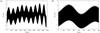 |
Fig. 1 Librational response times the mean radius of the icy shell of Europa by taking into account the orbital perturbations over 4500 days a) and a zoom over 800 days b). The amplitude increase in panel a) is due to the contribution of long-periodic Fourier terms with different phases. The initial date for the plot is January 1st 2026 corresponding to the expected date of arrival of EJSM at Jupiter. The interior model comes from the Table 4. |
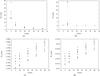 |
Fig. 2 Variation, with shell thickness (h), of the amplitude multiplied by the mean radius for the 4 main librations, 3.52 days a), 7.05 days b), 482 days c), and 485 days d). |
Resulting libration for Europa due to orbital forcing.
The librational response driven by the external torque exerted by Jupiter on Europa is obtained from Eqs. (12)–(13) for the orbital perturbations (Table 1). We first calculate the librations for the interior structure of Europa composed of a solid interior (core plus mantle), a water ocean, and a solid icy shell listed in Table 4. The temporal behavior of the libration from January 1st 2026, date of expected arrival EJSM, is shown in Figs. 1a,b over 4500 and 800 days, respectively. The main libration is seen to have a short period but its amplitude appears to be strongly modulated on long periods of about 480 days. The short-period libration has an amplitude of about 200″ corresponding to a surface displacement at the equator of 1.4 km and the long period of 480 days has almost the same amplitude. Here, the amplitude is given as a surface displacement at the equator by multiplying the libration angle by the mean radius of the satellite.
A deeper insight into the motion is obtained by analyzing directly the librational motion in frequency domain. Table 6 lists the physical librations in order of decreasing amplitude. The main libration is a 3.52 days oscillation, i.e. the mean mean longitude of Europa perturbed by Io (L1 − L2). The forcing for this term is mainly related to the eccentricity of the orbit (see Sect. 3). Next, librations associated with long periods of 482.06 days, 485.60 days, and 462.51 days, which are related to the precession of the nodes of the orbits of satellites (ν + ϖk where k stands for each Galilean satellites), have amplitudes around 70 and 10% smaller than the main term. The influence of the resonant interactions and the Sun are the 5th and 6th most important librations. We also note the presence of the L2 − L3 oscillation, with a period approximatively twice the orbital period, although its magnitude is relatively small.
The comparison of the magnitude of the forcing terms in Table 1 and the amplitude of librations in Table 6 shows that for the low frequency (long period) terms the forcing
magnitude Hj and the libration amplitude
 are similar
whereas the amplitudes of the high frequency (short period) terms are strongly diminished
with respect to the forcing. The separation between high and low frequencies is with
respect to the proper frequencies and is due to the presence of the forcing frequency in
the denominator (Eq. (13)), which
decreases the libration amplitude for short periods. This dynamical behavior corresponds
to the dynamics of a coupled forced oscillator where the restoring force is Jupiter’s
gravitational torque, the coupling force is
Kint(γs − γi),
and the moons inertia is
are similar
whereas the amplitudes of the high frequency (short period) terms are strongly diminished
with respect to the forcing. The separation between high and low frequencies is with
respect to the proper frequencies and is due to the presence of the forcing frequency in
the denominator (Eq. (13)), which
decreases the libration amplitude for short periods. This dynamical behavior corresponds
to the dynamics of a coupled forced oscillator where the restoring force is Jupiter’s
gravitational torque, the coupling force is
Kint(γs − γi),
and the moons inertia is  approximated as
  for quasi-periodic
librational response (Eqs. (9) and (10)). For small frequencies, the gravitational
torque is dominant and the orientation of the moon follows the direction of the force by
keeping the same face toward Jupiter, i.e. the amplitude of the libration
(γl for
l = s,i) equals to the magnitude of the longitude
perturbation (v) and hence
ψs = 0
(ψs = v − θs
defined in Sect. 2). We note that in this case the coupling torque vanished since the
three angles
(γs,γi,v)
are in phase. On contrast, for high frequency oscillations the inertia of the moon has a
strong impact and the moon does not orient its long axis toward Jupiter anymore. This
behavior is similar to the case of Enceladus (Rambaux et al. 2010).
for quasi-periodic
librational response (Eqs. (9) and (10)). For small frequencies, the gravitational
torque is dominant and the orientation of the moon follows the direction of the force by
keeping the same face toward Jupiter, i.e. the amplitude of the libration
(γl for
l = s,i) equals to the magnitude of the longitude
perturbation (v) and hence
ψs = 0
(ψs = v − θs
defined in Sect. 2). We note that in this case the coupling torque vanished since the
three angles
(γs,γi,v)
are in phase. On contrast, for high frequency oscillations the inertia of the moon has a
strong impact and the moon does not orient its long axis toward Jupiter anymore. This
behavior is similar to the case of Enceladus (Rambaux et al. 2010).
5.2. Influence of geophysical parameters
Figure 2a shows that the main geophysical parameter
that drives the libration at the orbital frequency is the thickness of the icy
shell h (Van Hoolst et al. 2008). Here a similar hyperbolic behavior dependence of libration amplitude on
shell thickness is obtained for the libration at 7.05 days (Fig. 2b). On contrast, the amplitudes of the librations at 482 days and
485 days depend only very weakly on shell thickness (see Figs. 2c,d), in accordance with the observation above that the libration
amplitude at low frequency is almost equal to the restoring force, i.e. Jupiter’s
gravitational interaction, magnitude. By introducing the condition that the forcing
frequency
ωj ≪ ω1,ω2
in the librational solution (Eq. (12)), the libration amplitude of the shell can be
approximated correct up to the third order in
ωj as 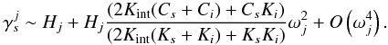 (15)where the
Kj
(j = i,s) are defined in the Appendix A and depend on
interior parameters. At first order in ωj,
the amplitude is equal to
the forcing magnitude Hj. The small
dependence on the interior is given by the coefficient of the term in the square of the
forcing frequency. The dependence on h is very weak, with differences in
amplitude of the order of a meter (Figs. 2c, d) that
is too small to be observed. Therefore, it will be not possible to obtain information on
the interior by measuring these long-period librations.
(15)where the
Kj
(j = i,s) are defined in the Appendix A and depend on
interior parameters. At first order in ωj,
the amplitude is equal to
the forcing magnitude Hj. The small
dependence on the interior is given by the coefficient of the term in the square of the
forcing frequency. The dependence on h is very weak, with differences in
amplitude of the order of a meter (Figs. 2c, d) that
is too small to be observed. Therefore, it will be not possible to obtain information on
the interior by measuring these long-period librations.
The amplitude of high frequency librations (Figs. 2a,b) depends not only on the magnitude of the coupling
(Hj in Eq. (11)) but also on the proximity of the forcing frequency
(ωj) to the eigenvalues of the proper modes
ω1 and ω2 as shown in Eq. (13). Whereas ω2
(between 2π/52 and 2π/60 days-1 for our
models) is far from the forcing frequencies, ω1 can be close
to the largest frequencies for small shell thickness (Fig. 3). For small thickness of the
icy shell the proper period (2π/ω1) tends
toward a few days (Fig. 3), i.e. very close to the
forcing periods of 7.05 days and 3.52 days, and leads to the resonance shape curves shown
in Figs. 2a,b. For the 7.05 days libration the
increase is significant because the resonance is crossed for
h ~ 10 km. In the linear model developed in Sect. 2 the
amplitude tends toward infinity that is contrary to the hypothesis of small libration
amplitude. In order to compare with a more realistic libration model at the resonance, we
numerically integrated the non-linear Eq. (2). The resulting libration is shown with red triangles. Outside the resonance
both results coincide and the difference appears only at the resonance as expected. The
two lines of resonance (blue and violet) have been computed by assuming that only
Bs − As
and Cs depend on h and
keeping all other geophysical parameters constants. In this case, the amplitude can be
expressed as 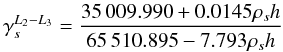 (16)where
ρs is the density of the shell expressed
in kg/m3 and the icy thickness h is expressed in km. The
blue dashed curve is plotted for a density equal to 800 kg/m3 while the violet
line is plotted for a density of 1000 kg/m3. These curves highlight the
importance of the shell density on the position of the resonance (in the frequency space).
Therefore, the amplitude of the libration is sensitive to the icy
thickness h and to the density of the ice shell because the last
parameter controls the position of the resonance.
(16)where
ρs is the density of the shell expressed
in kg/m3 and the icy thickness h is expressed in km. The
blue dashed curve is plotted for a density equal to 800 kg/m3 while the violet
line is plotted for a density of 1000 kg/m3. These curves highlight the
importance of the shell density on the position of the resonance (in the frequency space).
Therefore, the amplitude of the libration is sensitive to the icy
thickness h and to the density of the ice shell because the last
parameter controls the position of the resonance.
The observational determination of the two librations at 3.52 and 7.05 days might separate the contribution of the icy thickness h and icy density ρs. These two geophysical parameters are crucial for geophysical, geological, and astrobiological studies of Europa. The presence of a resonance in the librational motion of Europa may increase significantly the oscillatory motion of the satellite and thus tidal heating and surface faulting of the moon. However, to determine the amplitude of librations in resonance, the rotational model needs to take into account dissipative torques that will bound the highest amplitude and modify slightly the location of the resonance. In the available observations no signature of such dramatic events have been found but it cannot be ruled out that today or during its history Europa has reached such resonance. Hussmann & Spohn (2004) showed that the icy thickness of Europa may vary during time due to the variation of the eccentricity and may have reached values as small as 3 km.
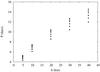 |
Fig. 3 Variation of the period of the eigenvalue of the first proper mode for Europa. |
6. Ganymede’s librations
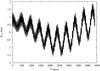 |
Fig. 4 Librational response times the mean radius of Ganymede from orbital perturbations. The main libration is an oscillation at the longitude of the Sun period. The initial date for the plot is January 1st 2026. |
Resulting libration for Ganymede due to orbital forcing.
In contrast to Europa, Ganymede’s largest libration is due to solar perturbations Ls and is not of orbital period (Fig. 4 and Table 7) because Ganymede is further away from Jupiter. As can be seen in Table 7, the second to fourth largest libration terms are due to the precession of the nodes ν + ϖm with m = 2,3,4. The libration in longitude at the orbital period 7.15 days is only the 6th largest term and is almost 3.8 times smaller than the main term. We recall that this mode is essentially due to the eccentricity of the orbit (see Sect. 3). In the case of Ganymede the eccentricity is around 0.0013, about a factor 7 smaller than the eccentricity of Europa (0.0094). Since the long-period librations are dominant, a complete study of the librational motion of Ganymede including the long-period librations is clearly required for any rotational data analysis of Ganymede.
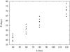 |
Fig. 5 Variation of the period of the first eigenvalue of the proper mode for Ganymede. For an icy shell of thickness equal to 60 kilometers, the proper mode is of the order of 50 days that is very close to the forcing mode of L3 − 2L4 + ϖ4 and leads to a large resonance effects. |
As explained for Europa, the amplitude of the long-period librations almost does not depend on the existence of a subsurface ocean and can therefore not be used to study the interior structure of Ganymede. The dependence of the libration at orbital period on the thickness h of the icy shell for Ganymede is similar to the case of Europa (see also Baland & Van Hoolst 2010). Of particular interest here is that the libration with a period of 50 days associated with the forced libration L3 − 2L4 + ϖ4 related to the interaction with Callisto may be resonant with the first proper mode, which has a period tending toward 50 days for an icy shell thickness of h ~ 60 kilometers (Fig. 5). Such a resonance might lead to a large libration amplitude at that period if the forced and proper frequencies coincide.
Resulting libration for Callisto due to orbital forcing.
Amplitude of the main librations of Europa, Ganymede, and Callisto.
7. Callisto’s librations
The most distant satellite of the Galilean moons is Callisto and contrary to Io, Europa, and Ganymede, it is not involved in the Laplace resonance. Therefore, its libration series (Table 8) is dominated by the Sun perturbations (at 4332 days) and there are no components containing the great inequality. The behavior of the librational response of Callisto is shown in Fig. 6 with the geophysical parameters listed in Table 4. The second main libration is the long period of − ϖ3 + ϖ4 − Ω3 + Ω0. The third oscillation is the libration in longitude at the orbital period related to the eccentricity. Its amplitude is almost 10 times smaller than the main term. The long-period librations are even more dominant than for Ganymede and Europa due to Callisto’s larger distance from Jupiter.
The long period behavior is similar to that for Europa and Ganymede in the sense that the amplitudes of long-period librations are close to the magnitudes of the forcing terms. However, in the short period regime a resonance with a proper mode does not seem to be possible. The proper periods are in the range of 250–550 days for P1 and 775–1175 days for P2, which are far from any forcing frequency.
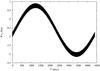 |
Fig. 6 Librational response multiplied by the mean radius of Callisto from orbital perturbations. The main libration is a long period at 4332 days due to the Sun orbital perturbation. The initial date for the plot is January 1st 2026. |
8. Discussion and conclusion
In this paper, we have studied the effect of orbital perturbations on the librational response of Europa, Ganymede, and Callisto. The orbital perturbations are induced by mutual gravitational interactions among satellites, especially the resonant interactions related to the Laplace resonance for Europa and Ganymede, and the solar gravitational interaction. These perturbations, which have been determined from the most recent numerical ephemerides of the Galilean moons (Lainey et al. 2006), introduce a wide range of frequencies in the librations. The resulting librations can be classified in two groups depending on the value of the frequencies with respect to the proper frequencies. For small frequencies, the restoring torque is dominant and the moons librate by keeping the same face toward Jupiter in phase with the perturbations. The resulting amplitude is almost equal to the magnitude of the orbital perturbations (at first order in frequencies). For the second group, the frequencies are long and around the orbital frequency. In this case, the inertia of the moon plays an important role and the amplitude is reduced with respect to the magnitude of the perturbations. Nevertheless, they can be strongly increased by a resonance between a proper frequency and forced frequencies. The limit between the short and long periods is essentially controlled by the highest proper frequency (ω1).
The short-period libration amplitudes may increase in the presence of a subsurface oceans as shown in Table 9. The observed libration amplitude depends on the strength of the external torque and are modified by the internal structure. They would provide information on the exact coupling mechanisms between the shell and the interior and can be used to better model satellite’s interior. In contrast to previous studies, which only considered libration at orbital period, we used the whole spectrum of the Galilean satellites to study the dependence of librations on the internal structure. In particular for Europa, we identified a second short-period libration at twice the orbital period, whose amplitude, although an order of magnitude smaller than the amplitude of the libration at 3.52 days, could also be used to infer information on the thickness and density of the icy shell relevant for geophysical, geological, and astrobiological studies (Eq. (16)).
The long-period librations are related to the orbital motion of Jupiter around the Sun with a period of 4332 days and to the motion of the orbital nodes and great inequality ν, leading to periods of ~480 days. In contrast to the high frequency librations, the amplitude of the small frequency librations does almost not depend on the distribution of mass inside the satellites. As a consequence, this result is robust and does not depend on the coupling mechanisms. In addition, it is important to underline that an adequate description of the rotational motion of the satellites requires to take into account the long-period librations because their amplitudes are not negligible and even dominant for Ganymede and Callisto. If such librations are neglected in the reduction process, the fitted rotational speed will be increased (or decreased depending on the phase) leading to a misstatement of non-synchronous rotation of satellites.
The oscillatory motions of the icy Galilean moons present a wide spectrum of frequencies due to orbital perturbations. Some of the librations may present large amplitudes due to a resonance with one of the proper modes. The exact position of the resonance in frequency space, i.e. the value of the proper frequencies, is sensitive to the values of the geophysical parameters introduced in our model. By exploring a large range of possible values of structure parameters, we have shown that such resonances might exist for Europa and Ganymede for realistic ranges of parameters. Although no observational evidence is available for a resonant libration for Europa or Ganymede, it cannot be ruled out that these bodies have crossed a libration resonance during their histories, leading to potential surface faulting and increased tidal heating.
In the present libration model, we have taken into account the gravitational torque exerted by Jupiter and both pressure and internal gravitational couplings, but neglected (visco-)elastic effects. The largest elastic effect can be expected to be due to the tidal forcing of Jupiter and, by analogy to solid rotation, it could contribute up to 10% to the libration amplitude at orbital frequency (Baland & Van Hoolst 2010). The effect of inelastic tides on libration is most likely very small, as shown e.g. for Enceladus (Rambaux et al. 2010) without liquid ocean. Viscous relaxation of the ice shell is also thought not to be efficient in changing the libration because it is too slow for short periodic librations and not effective for the long-period librations for which the satellites always keep the same face toward Jupiter (see Sect. 5). In addition, friction at the shell/ocean interface and flow in the ocean (Noir et al. 2009; Tyler 2008) could modify the amplitude of the librations.
The librational motion of the Galilean satellites may be inferred by spacecraft measurements by tracking surface landmarks, by fitting the shape of the satellites from surface images (Tiscareno et al. 2010), and/or by altimeter measurements. The accuracy obtained in the pole location of Titan from the different flybys by the radar Cassini instrument is below 1 km. However, Wu et al. (2001) predicted for Europa an accuracy of 0.02 km with 15 days of tracking from 2 Earth stations of an Europa orbiter. At such level of precision (2.8″) all librations presented in Table 6 may be detected. Let us mention that there is not yet enough powerful techniques to reach the Galilean moons directly from the Earth as one for Mercury by radar interferometry (Margot et al. 2009) or the Moon by Lunar Laser Ranging (Williams et al. 2001) but we could expect that some techniques will be improved in the near future.
Acknowledgments
N.R. thanks V. Lainey for fruitful discussions on the orbital ephemerides of Galilean satellites.
References
- Baland, R. M., & Van Hoolst, T. 2010, Icarus, in press [Google Scholar]
- Blanc, M., Alibert, Y., André, N., et al. 2009, Exp. Astron., 23, 849 [NASA ADS] [CrossRef] [Google Scholar]
- Billings, S. E., & Kattenhorn, S. A. 2005, Icarus, 177, 397 [NASA ADS] [CrossRef] [Google Scholar]
- Bills, B. G. 2005, Icarus, 175, 233 [NASA ADS] [CrossRef] [Google Scholar]
- Comstock, R. L., & Bills, B. G. 2003, J. Geophys. Res. Planets, 108, 5100 [NASA ADS] [CrossRef] [Google Scholar]
- Danby, J. M. A. 1988, Fund. Celest. Mech. (Willman-Bell Inc.) [Google Scholar]
- Ferraz-Mello, S. 1979, Dynamics of the Galilean Satellites, Mathmematical and Astronomical Series, 1 [Google Scholar]
- Gastineau, M., & Laskar, J. 2008, trip 0.99, Manuel de référence TRIP, Paris Observatory, http://www.imcce.fr/Equipes/ASD/trip/trip.html [Google Scholar]
- Greenberg, R. 2005, Europa the Ocean Moon (Springer) [Google Scholar]
- Henrard, J. 2005a, Celest. Mech. Dynam. Astron., 91, 131, 149 [Google Scholar]
- Henrard, J. 2005b, Celest. Mech. Dynam. Astron., 93, 101 [Google Scholar]
- Henrard, J., & Schwanen, G. 2004, Celest. Mech. Dynam. Astron., 89, 181 [Google Scholar]
- Hussmann, H., & Spohn, T. 2004, Icarus, 171, 391 [NASA ADS] [CrossRef] [Google Scholar]
- Hussmann, H., Sohl, F., & Spohn, T. 2006, Icarus, 185, 258 [NASA ADS] [CrossRef] [Google Scholar]
- Jeffreys, H. 1952, The Earth, ed. Cambridge [Google Scholar]
- Kivelson, M. G., Khurana, K. K., Stevenson, D. J., et al. 1999, J. Astrophys., 104, 4609 [Google Scholar]
- Kivelson, M. G., Khurana, K. K., Russell, C. T., et al. 2000, Science, 289, 1340 [NASA ADS] [CrossRef] [PubMed] [Google Scholar]
- Kivelson, M. G., Khurana, K. K., & Volwerk, M. 2002, Icarus, 157, 507 [NASA ADS] [CrossRef] [Google Scholar]
- Khurana, K. K., Kivelson, M. G., Stevenson, D. J., et al. 1998, Nature, 395, 777 [NASA ADS] [CrossRef] [PubMed] [Google Scholar]
- Lainey, V., Duriez, L., & Vienne, A. 2006, A&A, 456, 783 [NASA ADS] [CrossRef] [EDP Sciences] [Google Scholar]
- Lainey, V., Arlot, J.-E., Karatekin, Ö., & van Hoolst, T. 2009, Nature, 459, 957 [NASA ADS] [CrossRef] [PubMed] [Google Scholar]
- Laskar, J. 1988, A&A, 198, 341 [NASA ADS] [Google Scholar]
- Laskar, J. 2005, in Frequency Map analysis and quasi periodic decompositions, ed. D. Benest, C. Froeschler, & E. Lega, Hamiltonian Systems and Fourier Analysis (Cambridge: Cambridge Scientific Publishers) [Google Scholar]
- Margot, J. L., Peale, S. J., Jurgens, R. F., Slade, M. A., & Holin, I. V. 2007, Science, 316, 710 [NASA ADS] [CrossRef] [PubMed] [Google Scholar]
- Noir, J., Hemmerlin, F., Wicht, J., Baca, S. M., & Aurnou, J. M. 2009, Phys. Earth Planet. Inter., 173, 141 [Google Scholar]
- Noyelles, B. 2009, Icarus, 202, 225 [NASA ADS] [CrossRef] [Google Scholar]
- Pappalardo, R. T., Belton, M. J. S., Breneman, H. H., et al. 1999, J. Geophys. Res., 104, 24015 [NASA ADS] [CrossRef] [Google Scholar]
- Peale, S. J. 1976, Icarus, 28, 459 [NASA ADS] [CrossRef] [Google Scholar]
- Rambaux, N., Castillo-Rogez, J. C., Williams, J. G., & Karatekin, Ö. 2010, Geophys. Res. Lett., 37, 4202 [NASA ADS] [CrossRef] [Google Scholar]
- Schubert, G., Anderson, J. D., Spohn, T., & McKinnon, W. B. 2004, Jupiter. The Planet, Satellites and Magnetosphere, 281 [Google Scholar]
- Sohl, F., Spohn, T., Breuer, D., & Nagel, K. 2002, Icarus, 157, 104 [NASA ADS] [CrossRef] [Google Scholar]
- Spohn, T., & Schubert, G. 2003, Icarus, 161, 456 [NASA ADS] [CrossRef] [Google Scholar]
- Tiscareno, M. S., Thomas, P. C., & Burns, J. A. 2009, Icarus, 204, 254 [NASA ADS] [CrossRef] [Google Scholar]
- Tyler, R. H. 2008, Nature, 456, 770 [NASA ADS] [CrossRef] [PubMed] [Google Scholar]
- Van Hoolst, T., Rambaux, N., Karatekin, Ö., Dehant, V., & Rivoldini, A. 2008, Icarus, 195, 386 [NASA ADS] [CrossRef] [Google Scholar]
- Van Hoolst, T., Rambaux, N., Karatekin, Ö., & Baland, R.-M. 2009, Icarus, 200, 256 [NASA ADS] [CrossRef] [Google Scholar]
- Wu, X., Bar-Sever, Y. E., Folkner, W. M., Williams, J. G., & Zumberge, J. F. 2001, Geophys. Res. Lett., 28, 2245 [NASA ADS] [CrossRef] [Google Scholar]
- Williams, J. G., Boggs, D. H., Yoder, C. F., Ratcliff, J. T., & Dickey, J. O. 2001, J. Geophys. Res. Planets, 106, 27933 [NASA ADS] [CrossRef] [Google Scholar]
Appendix A: Expression of the librational angles
We introduce the following notation:  and
and
 .
.
 (A.1)
(A.1) (A.2)
(A.2) (A.3)
(A.3) (A.4)
(A.4) (A.5)
(A.5) (A.6)
(A.6) (A.7)
(A.7)
All Tables
Selected interior model for Europa, Ganymede and Callisto. R and ρ are the radius and density of the different layers.
All Figures
|
Fig. 1 Librational response times the mean radius of the icy shell of Europa by taking into account the orbital perturbations over 4500 days a) and a zoom over 800 days b). The amplitude increase in panel a) is due to the contribution of long-periodic Fourier terms with different phases. The initial date for the plot is January 1st 2026 corresponding to the expected date of arrival of EJSM at Jupiter. The interior model comes from the Table 4. |
| In the text | |
|
Fig. 2 Variation, with shell thickness (h), of the amplitude multiplied by the mean radius for the 4 main librations, 3.52 days a), 7.05 days b), 482 days c), and 485 days d). |
| In the text | |
|
Fig. 3 Variation of the period of the eigenvalue of the first proper mode for Europa. |
| In the text | |
|
Fig. 4 Librational response times the mean radius of Ganymede from orbital perturbations. The main libration is an oscillation at the longitude of the Sun period. The initial date for the plot is January 1st 2026. |
| In the text | |
|
Fig. 5 Variation of the period of the first eigenvalue of the proper mode for Ganymede. For an icy shell of thickness equal to 60 kilometers, the proper mode is of the order of 50 days that is very close to the forcing mode of L3 − 2L4 + ϖ4 and leads to a large resonance effects. |
| In the text | |
|
Fig. 6 Librational response multiplied by the mean radius of Callisto from orbital perturbations. The main libration is a long period at 4332 days due to the Sun orbital perturbation. The initial date for the plot is January 1st 2026. |
| In the text | |
Current usage metrics show cumulative count of Article Views (full-text article views including HTML views, PDF and ePub downloads, according to the available data) and Abstracts Views on Vision4Press platform.
Data correspond to usage on the plateform after 2015. The current usage metrics is available 48-96 hours after online publication and is updated daily on week days.
Initial download of the metrics may take a while.