| Issue |
A&A
Volume 526, February 2011
|
|
|---|---|---|
| Article Number | A47 | |
| Number of page(s) | 5 | |
| Section | Astronomical instrumentation | |
| DOI | https://doi.org/10.1051/0004-6361/201015487 | |
| Published online | 20 December 2010 | |
Weeds: a CLASS extension for the analysis of millimeter and sub-millimeter spectral surveys
1
Laboratoire d’Astrophysique de Grenoble, Observatoire de Grenoble,
Université Joseph Fourier, CNRS, UMR 571
Grenoble,
France
e-mail: sebastien.maret@obs.ujf-grenoble.fr
2
Institut de Radioastronomie Millimétrique,
300 rue de la Piscine, 38406 Saint Martin d’Hères,
France
3
LERMA, UMR 8112, CNRS and Observatoire de Paris, 61 avenue de
l’Observatoire, 75014
Paris,
France
Received:
28
July
2010
Accepted:
6
December
2010
The advent of large instantaneous bandwidth receivers and high spectral resolution spectrometers on (sub-)millimeter telescopes has opened up the possibilities for unbiased spectral surveys. Because of the large amount of data they contain, any analysis of these surveys requires dedicated software tools. Here we present an extension of the widely used CLASS software that we developed to that purpose. This extension, named Weeds, allows for searches in atomic and molecular lines databases (e.g. JPL or CDMS) that may be accessed over the internet using a virtual observatory (VO) compliant protocol. The package permits a quick navigation across a spectral survey to search for lines of a given species. Weeds is also capable of modeling a spectrum, as often needed for line identification. We expect that Weeds will be useful for analyzing and interpreting the spectral surveys that will be done with the HIFI instrument onboard Herschel, but also observations carried-out with ground based millimeter and sub-millimeter telescopes and interferometers, such as IRAM-30 m and Plateau de Bure, CARMA, SMA, eVLA, and ALMA.
Key words: ISM: molecules / ISM: lines and bands / line: identification / methods: data analysis / virtual observatory tools
© ESO, 2010
1. Introduction
A spectral survey consists in a series of spectra covering a significant spectral domain. At (sub-)millimeter wavelengths, a spectral survey typically covers several tens of GHz. Spectral surveys are generally referred to as unbiased if they provide a complete coverage with a uniform sensitivity. As such, they allow for a complete census of the species emitting in that band, and sometimes for discovery of new interstellar species. In addition, because a given band often contains many transitions of the same species, the simultaneous analysis of all these lines provides stringent constraints on the physical conditions in the emitting gas, such as the density and temperature. Therefore spectral surveys are very useful for characterizing both the chemical composition and physical condition in the observed objects.
Ever since the pioneering work of Johansson et al. (1984), who carried-out an unbiased spectral survey of the Orion KL star-forming region and IRC +10216 carbon-rich star between 72 and 91 GHz with the Onsala telescope, many spectral surveys have been carried-out at millimeter and sub-millimeter wavelengths using ground-based telescopes (see Herbst & van Dishoeck 2009, for a review). Because of the limited sensitivity of the instruments available at that time, early spectral surveys were targeted at bright star-forming regions, such as Orion KL and Sgr B2 in the millimeter range. Thanks to the increasing sensitivity of heterodyne receivers and the availability of sub-millimeter telescopes, these surveys were later extended to higher frequencies (e.g. Schilke et al. 1997, 2001; Comito et al. 2005) and carried-out towards fainter young stellar objects (e.g. NGC 1333 IRAS4 or IRAS16292-2422; Blake et al. 1994; van Dishoeck et al. 1995; Blake et al. 1995). A few spectral surveys have been carried with millimeter and sub-millimeter interferometers, such as OVRO or the SMA (e.g. Blake et al. 1996; Beuther et al. 2006). The HIFI instrument (de Graauw et al. 2010) onboard the Herschel space observatory (Pilbratt et al. 2010) now allows for a complete coverage of the almost unexplored 480–1250 and 1410–1910 GHz frequency bands. Its large spectral coverage – up to 4 GHz instantaneous bandwidth – and unprecedented sensitivity in this frequency range enable astronomers to carry-out spectral surveys over almost 1.5 THz down to the line confusion limit in a few tens of hours. The first spectral surveys with this instrument have already given spectacular results (Bergin et al. 2010; Ceccarelli et al. 2010). Among these, we can cite the richness of the Orion BN-KL spectrum observed at THz frequencies (see Fig. 2, Bergin et al. 2010) or the discovery of ND in IRAS16293-2422 (Bacmann et al. 2010).
Current developments in (sub-)millimeter instruments include an increase in the instantaneous bandwidth of the detection devices. During the past decade, the instantaneous bandwidth of tunable heterodyne receivers has increased by more than an order of magnitude, now routinely reaching ~10 GHz. Other technologies (e.g. HEMT, FCRAO and IRAM) have already provided several tens of GHz, although it is still unclear whether the sensitivity of these receivers can match that of SIS receivers. This increase in bandwidth has been accomplished in parallel with the advent of digital spectrometers (autocorrelators, fast Fourier transform), the versatility of which allow the coverage of such bandwidth with a spectral resolution down to a few hundred kHz. As a result, unbiased spectral surveys of the 3 mm atmospheric window (ν = 80−117 GHz) can be done with the IRAM-30 m telescope in ~10 h, with a 2 mK noise at 1σ in 2 MHz (~6 km s-1) spectral channels. The ALMA interferometer will also permits coverage of large frequency windows, providing spectral cubes with up to 8 GHz bandwidth (Wootten 2008). Thanks to its sensitivity, this instrument will allow, in its compact configuration, line surveys to be carried-out down to the confusion limit toward a large number of sources. Spectral surveys are thus still in their infancy and will very likely become routine observing modes in the coming years.
Spectral surveys covering large frequency bands require specific tools to be analyzed efficiently. In this article, we present a software that is intended for the analysis of spectral surveys. In Sect. 2, we briefly describe how such surveys are analyzed. In Sect. 3 we detail how our software was designed and implemented to carried-out such an analysis. Finally Sect. 4 concludes this article and discuss future developments.
2. Spectral surveys analysis
The analysis of a spectral survey usually consists in identifying the various lines and in deriving the physical and chemical properties of the emitting gas (density, temperature and column densities of the observed species). The main difficulty in such identification is that large molecules may have hundreds of lines in the (sub-)millimeter range. These species – such as methanol, methyl formate or dimethyl ether – are often named weeds by spectroscopists. If the lines are too broad, they may overlap and blend together, which makes the identification of weaker lines difficult. This is the line confusion limit (Schilke et al. 1997): line identification is not limited by the signal-to-noise of the observations, but by the line blending.
Because of this problem, extreme care must be taken when identifying species from a spectral survey. Herbst & van Dishoeck (2009) summarize the criteria for a firm detection as follows: “(i) rest frequencies are accurately known to 1:107, either from direct laboratory measurements or from a high-precision Hamiltonian model; (ii) observed frequencies of clean, nonblended lines agree with rest frequencies for a single well-determined velocity of the source; if a source has a systematic velocity field as determined from simple molecules, any velocity gradient found for lines of a new complex molecule cannot be a random function of transition frequency; (iii) all predicted lines of a molecule based on an LTE spectrum at a well-defined rotational temperature and appropriately corrected for beam dilution are present in the observed spectrum at roughly their predicted relative intensities. A single anticoincidence (that is, a predicted line missing in the observational data) is a much stronger criterion for rejection than hundreds of coincidences are for identification. This last criterion is one of the strongest arguments for complete line surveys rather than targeted line searches”.
The rest frequencies needed to fulfill criterion (i) are usually taken from spectral lines catalogs, such as the Cologne Database for Molecular Spectroscopy (CDMS, Müller et al. 2001) or the JPL Molecular Spectroscopy catalog (Pickett et al. 1998). For criterion (ii), we need to compare the consistency of the centroid velocities of all the line candidates. Finally criterion (iii) requires to perform a model of the predicted emission of the given species so that it can be compared with the observations. The traditional technique for this consist in building a rotational diagram (Goldsmith & Langer 1999) to see if all detected lines agree with a single rotational temperature and column density. Alternatively, one can compute synthetic spectrum and compare it directly with the observations – a technique called forward fitting (Comito et al. 2005). This approach is also extremely useful when one wants to search for weak lines of a specie among hundreds from various weeds: a synthetic spectrum of the emission of the weeds can be constructed to fit the observed transitions in an iterative fashion. Once the brightest lines have been modeled, one can compare the synthetic spectrum to the observed one to look for lines from less abundant species (see Belloche et al. 2008, for an example of this technique). Of course, this also allows the physical and chemical properties of the emitting gas to be derived.
Since spectral surveys may contain thousands of lines, they require specific tools to be efficiently analyzed. Two packages have been developed for that purpose. The first of them, XCLASS (Schilke et al. 2001), is an extension of the widely used CLASS data reduction software, which is part of Gildas. XCLASS contains a spectral line database which is built from the CDMS and JPL catalogs. Technically, it uses the MySQL database server which must be installed on the user computer. This database may be updated manually, by replacing the database file by the one provided by the program authors. XCLASS allows the user to look for lines corresponding to a given frequency in its catalog, but also to make a model at the LTE of the observed spectra. XCLASS has been successfully used to reduce several spectral surveys obtained with the CSO and the IRAM-30 m (Schilke et al. 2001; Comito et al. 2005; Belloche et al. 2008). However, XCLASS is based on an obsolete version of CLASS, which is not maintained anymore. Indeed, the CLASS internal structures was largely rewritten in 2005–2006 to adapt to the challenges of data reductions coming with the recent generation of receivers (Hily-Blant et al. 2005). The second package, CASSIS, has been developed primarily to analyze Herschel-HIFI spectral surveys, although it can be used to analyze surveys from ground based telescopes as well. CASSIS itself does not have data reduction capabilities; therefore data must first be reduced in another software such as CLASS or HIPE (Ott et al., in prep.) before analysis in CASSIS. CASSIS uses a database which is built from the CDMS and the JPL catalog; in recent CASSIS versions, this database (SQLite) is embedded in the program so that an external database server is no longer required. Like XCLASS, CASSIS allows the forward-fitting of a spectrum, but also the search for the various transitions of a given specie.
3. Weeds design and implementation
3.1. General design
Weeds has been designed specifically to analyze spectral surveys, following the approach presented in Sect. 2. Although its development was inspired by the XCLASS and CASSIS packages, it is different in several aspects. Weeds is an extension of the current version of the CLASS software, and is mostly written in Python language, except for a few command written in the Gildas command interpreter (SIC) language. To do this, Weeds uses the new possibility offered by GILDAS to interleave Python and SIC in the same session (Bardeau et al. 2010). In particular, the variable contents are shared between Python and SIC. Python has several advantages over other languages for developing such extensions. It benefits from a large library of modules that allow complex tasks – such as making a query in a VO-compliant database, see Sect. 3.2 – to be done relatively easily. Although it is interpreted, it is still computationally efficient, because critical modules (e.g. the module for array computations that we use for the spectra modeling, see Sect. 3.4) are written in compiled languages such as C or Fortran. Weeds is distributed with Gildas since April 2010. The source code is freely available from the IRAM website1. A user manual is also available on that page.
Because Weeds is an extension of CLASS, it can be used to analyze any data format that CLASS supports. In practice, the CLASS data format is used by many ground-based telescopes (e.g. IRAM-30 m, CSO and APEX). Data from other telescopes can be converted to FITS format and imported into CLASS as well. For example, Herschel-HIFI can be imported into CLASS through the FITS filler delivered by the HIPE data reduction software (Delforge et al., in prep.). In order to analyze data in Weeds, the data must have been calibrated and reduced first. The reduction usually consists in flagging the bad channels, averaging the scan covering the same frequency range together, and removing a polynomial baseline. If the data were obtained with double sideband (DSB) receiver, sideband deconvolution might be needed in order to produce a SSB spectrum. This requires a special observing technique, i.e. a number of overlapping spectra with shifted local oscillator frequency. Deconvolution can then be performed in CLASS using the algorithm developed by Comito & Schilke (2002). Thus data reduction and analysis can be done within the same environment.
3.2. Spectral line catalogs queries
As mentioned above, line identification requires repeated queries to spectral lines catalogs, such as the CDMS or the JPL. Unlike XCLASS and CASSIS – who require a custom catalog installed on the user’s computer – Weeds performs queries in spectral line databases through the Internet2. This has the advantage of not requiring any update of a custom catalog: changes in the database, such as species addition or line frequency corrections or updates, are readily available in Weeds. In order to make queries in spectral lines catalogs, we have implemented the VO-compliant Simple Line Access Protocol (SLAP, Salgado et al. 2009) in Weeds. This protocol allows spectral line databases queries to be made in a standardized way; any database that implements the protocol can be accessed by Weeds. Because it is a VO standard, it is likely that more and more spectral line database will use it in the future. Nonetheless, as of this writing only the CDMS is accessible using that protocol, through an interface at the Paris VO Observatory (Moreau et al. 2008). Therefore, in order to access the JPL catalog from Weeds, we have implemented queries in the specific protocol which is used by this database. The CDMS can be accessed through its own protocol as well.
For the moment, only one database can be used at a time; it is not possible to combine the catalogs, i.e. to use species some out the JPL and some out the CDMS. In the future, the VAMDC project3 will provide a single, unified database, including state-of-art spectroscopic data from both the CDMS and the JPL catalogs. We plan on implementing an access to this database from Weeds as soon as it it released.
From the user point of view, Weeds provides a command to search for lines corresponding to a given frequency range in a spectral line catalog. The user can select a region on the spectrum displayed in CLASS, and the command prints all the lines from the catalog around the region selected. The lines can be filtered out on the basis of the species they belong to, their Einstein coefficient, or their upper level energy. For double sideband spectra, a command option allows the search for lines from the image band.
3.3. Lines browsing/identification
To secure the detection of a species in a spectral survey, one needs, according to criterion (ii) to search for all the transitions of that species in the entire frequency range covered by the survey. One also needs to measure the velocity of each line to check that they correspond to a single velocity. Weeds allows the user to browse through a survey rapidly. For this, Weeds has a command to search for all the lines of a given specie that fall in the frequency range covered by the survey. The command prints the lines in the terminal, but also builds an internal index containing all these lines, that we can order either by increasing frequency or increasing upper level energy. Another command allow the user to examine each of the line candidate one by one, to see if the line is detected or not. This command makes a zoom on a small frequency region around the (expected) line, and also sets the velocity scale with respect to the rest frequency of the line. A vertical mark is also drawn on the displayed spectrum at the source velocity, so that we can easily determine if the line is detected or not. A Gaussian fit of the observed line may be performed to determine the velocity of each line.
3.4. Spectra modeling
Once several transitions of a given specie have been found, one needs to check if the relative intensities of these components agree with a single excitation temperature (criterion (iii)). In addition, one needs to make sure that non-detected lines are consistent with the excitation temperature derived from other species – or in other words, that no lines are “missing”. For this Weeds allows the user to compute a synthetic spectrum that can be compared directly with the observations (forward-fitting). Following the approach used in XCLASS and described in Comito et al. (2005) the synthetic spectrum is computed assuming that the emission arises from one or several components at the LTE. Although this approximation is simplistic – it is well known that in the interstellar medium species are often out of local thermodynamic equilibrium, and many sources are known to have density and temperature gradients – yet such a zeroth-order approach is often extremely useful to identify lines, as mentioned above. Once the lines have been identified, a more realistic modeling, taking into account non-LTE excitation effects as well as the source structure, can be carried-out.
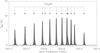 |
Fig. 1 Spectra between 524.2 and 525.5 GHz observed towards Orion-KL with Herschel-HIFI (filled histogram) and LTE model produced with Weeds (continuous black line). The rest frequencies of several detected methanol lines are indicated. |
Under these assumptions, and after baseline subtraction, the brightness temperature of a given species as a function of the rest frequency ν is given by: ![\begin{equation} \label{eq:1} T_\mathrm{B} \left( \nu \right) = \eta \left[ J_\nu \left( T_\mathrm{ex} \right) - J_\nu \left( T_\mathrm{bg} \right) \right] \left( 1 - {\rm e}^{-\tau \left( \nu \right)} \right) \end{equation}](/articles/aa/full_html/2011/02/aa15487-10/aa15487-10-eq7.png) (1)where η is beam dilution factor, which, for a source with a Gaussian brightness profile and a Gaussian beam, is equal to:
(1)where η is beam dilution factor, which, for a source with a Gaussian brightness profile and a Gaussian beam, is equal to:  (2)where θs and θt the source and telescope beam FWHM sizes, respectively. For a sake of simplicity, the latter is assumed to be given by the diffraction limit4
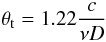 (3)where c is the light speed and D is the diameter of the telescope. Tbg is the brightness temperature of the background emission, i.e. the physical temperature that would have a black body producing the same background continuum emission (e.g. 2.73 K for the cosmic microwave background). Tex is the excitation temperature, and the opacity
  is:
is: 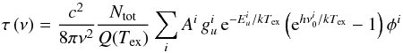 (4)where the summation is over each line of the considered species. Here Ntot is the total column density of the species considered, Q(Tex) is the partition function, Ai is the Einstein coefficient of the i line,
  and Eu are the upper level degeneracy and energy of the i line, and φi is the i line profile function. The latter is given by:
 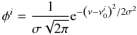 (5)where
  the is i line rest frequency and σ the line width in frequency units at 1/e. σ can be expressed as a function of the line FWHM in velocity units ΔV as follows:
  (6)Note that some of the model parameters may be degenerate in certain cases. In the optically thick or thin limits, the source size and temperature or the size and column density are degenerate, respectively (see Eqs. (1) and (3)). This degeneracy can be usually lifted if both thick and thin lines are present in the survey, or if lines from an rare isotopologue are detected together with the main one (e.g. 13CH3OH and CH3OH). The source size may also be constrained from interferometric observations.
Several components with e.g. different kinetic temperature or column density can be included in the computation. For this, we assume that the various components are not coupled radiatively – that is a photon from one component can not be absorbed by a another, foreground component – in which case the emerging spectrum is simply the sum of the brightness temperature of each components given by Eq. (1). Each of these component can be Doppler-shifted with respect to each other, which is useful when modeling sources with several components at different velocities. It is also possible to compute the spectra from several species; this is done by a summation of Eq. (1) over each specie.
The column densities, kinetic temperatures, Doppler width and source sizes for each species and components are read from a text file. Einstein coefficients, upper level degeneracy and energies as well as the partition functions are taken from spectral line catalogs. Because these catalogs usually give the partition functions at a few temperatures only, the partition function at the user temperature is computed from a linear interpolation (or extrapolation if the user given temperature is outside the range of temperature provided in the catalog). When computing the synthetic spectrum, a frequency sampling corresponding to the minimum ΔV divided by 10 is taken (or a frequency sampling equal to that of the observed spectra, if it smaller than the minimum ΔV divided by 10). This ensures that the sampling at all frequencies and for all species and components is sufficient. At the end of the computation, the synthetic spectrum is re-sampled to the same channel spacing than the observed spectrum in order to take the channel dilution factor into account. This allows for a direct comparison between the synthetic and observed spectra.
In Fig. 1, we show an example of such a modeling. The figure shows a spectrum between 524.2 and 525.2 GHz observed towards Orion-KL with Herschel-HIFI as part of the HEXOS guaranteed time key program (Bergin et al. 2010). These data have been already presented by Wang et al. (2010). Several methanol lines are detected. On this figure we show model predictions computed with a Weeds for a single component source with N(CH3OH) = 2 × 1017 cm-2, θS = 18″, T = 80 K and ΔV = 4 km s-1, and using the JPL database. Overall, the model predictions are in good agreement with the observations – in particular, we reproduce successfully the relative intensity of the brightest lines. On the other hand, this simple model underestimates the small line at 524 620 MHz and the shoulder at 524 880 MHz, maybe suggesting several emitting components and/or non-LTE excitation. Note that for the given parameters the emission is predicted to be optically thin, so that the column density and source size can not be constrained independently. A complete analysis of the methanol emission in this source is clearly beyond the scope of this paper; however this example demonstrates how a simple LTE model is useful to identify lines in a spectral survey. Finally, we have crossed-checked these model predictions with CASSIS and two packages were found to be in excellent agreement.
4. Conclusions and prospects
We have presented an extension of the CLASS data reduction software for analyzing spectral surveys. This extension allows the user to make queries in spectral line databases using a VO compliant protocol. It also allows the user to quickly search for the various transitions of a given specie. Finally it can compute model predictions at the LTE, as often needed to identify lines in spectra close to the confusion limit. Weeds has already been successfully used to analyze part of the IRAS 16293-2422 survey obtained with Herschel-HIFI (Bacmann et al. 2010; Hily-Blant et al. 2010), and we expect that it will be useful for future spectral surveys with this instrument as well. We think that it will become a standard tool for analyzing spectral surveys obtained with single dish ground based telescopes such as the IRAM-30 m. Yet, Weeds is not limited to the analysis of single dish observations. It may be used to analyze spectral surveys obtained with interferometers as well, such as the IRAM Plateau de Bure, CARMA, the SMA, and the upcoming ALMA and eVLA interferometers. In fact, since Weeds is written in Python, it could be used from the Python based CASA software, that will be used by the eVLA and ALMA. However, analyzing ALMA data will be challenging, because these data will consist in large spectral cubes, i.e. essentially a spectral survey on large number of pixels. In fact, doing such an analysis by hand, i.e. identifying the various lines/species on each spectrum of map is probably impossible; this will require some automatic fitting tools to extract the relevant information (column densities and excitation temperature of the various species) as a function of position. Such tools require efficient minimization algorithms to fit a model with a large number of free parameters to the data. The development of such tools is already in progress (e.g. in XCLASS using the MAGIX minimization framework), and implementing these automatic fitting tools in Weeds would be desirable in the future.
(Sub-)millimeter telescopes usually have tapers that limit the power received in side-lobes. Because of this, the telescope beam size may be different that of a purely diffraction limited antenna of the same diameter. However, the difference between the two is usually small: at 100 GHz, the measured FWHM of the IRAM-30 m is 24.6″, while Eq. (3) gives 25.2″.
Acknowledgments
The authors would like to thank Peter Schilke and Emmanuel Caux for fruitful discussions on the analysis of spectral surveys. We are also grateful to Charlotte Vastel for helping us testing the LTE modeling done in Weeds against CASSIS, and to Shyia Wang for providing us the Orion-KL spectrum prior to publication. Finally, we wish to thank the persons in charge of maintaining and the CDMS, JPL and Paris VO databases; without their continuous efforts, the development of analysis software such as Weeds would not be possible. We are especially grateful to Holger Müller, Brian Drouin and Nicolas Moreau for their help in implementing access to these databases in Weeds.
References
- Bacmann, A., Caux, E., Hily-Blant, P., et al. 2010, A&A, 521, L42 [NASA ADS] [CrossRef] [EDP Sciences] [Google Scholar]
- Bardeau, S., Reynier, E., Pety, J., & Guilloteau, S. 2010, PYGILDAS: Interleaving Python and GILDAS, Tech. Rep., IRAM [Google Scholar]
- Belloche, A., Menten, K. M., Comito, C., et al. 2008, A&A, 482, 179 [NASA ADS] [CrossRef] [EDP Sciences] [Google Scholar]
- Bergin, E., Phillips, T., Comito, C., et al. 2010, A&A, 521, L20 [NASA ADS] [CrossRef] [EDP Sciences] [Google Scholar]
- Beuther, H., Zhang, Q., Reid, M. J., et al. 2006, ApJ, 636, 323 [NASA ADS] [CrossRef] [Google Scholar]
- Blake, G. A., van Dishoek, E. F., Jansen, D. J., Groesbeck, T. D., & Mundy, L. G. 1994, ApJ, 428, 680 [NASA ADS] [CrossRef] [Google Scholar]
- Blake, G. A., Sandell, G., van Dishoeck, E. F., et al. 1995, ApJ, 441, 689 [Google Scholar]
- Blake, G. A., Mundy, L. G., Carlstrom, J. E., et al. 1996, ApJ, 472, L49 [NASA ADS] [CrossRef] [Google Scholar]
- Ceccarelli, C., Bacmann, A., Boogert, A., et al. 2010, A&A, 521, L22 [NASA ADS] [CrossRef] [EDP Sciences] [Google Scholar]
- Comito, C., & Schilke, P. 2002, A&A, 395, 357 [NASA ADS] [CrossRef] [EDP Sciences] [Google Scholar]
- Comito, C., Schilke, P., Phillips, T. G., et al. 2005, ApJS, 156, 127 [NASA ADS] [CrossRef] [Google Scholar]
- de Graauw, T., Helmich, F., Phillips, T., et al. 2010, A&A, 518, L6 [Google Scholar]
- Goldsmith, P. F., & Langer, W. D. 1999, ApJ, 517, 209 [NASA ADS] [CrossRef] [Google Scholar]
- Herbst, E., & van Dishoeck, E. F. 2009, ARA&A, 47, 427 [NASA ADS] [CrossRef] [Google Scholar]
- Hily-Blant, P., Pety, J., & Guilloteau, S. 2005, CLASS Evolution: I. Improved OFT support, Tech. Rep., IRAM [Google Scholar]
- Hily-Blant, P., Walmsley, M., Pineau Des forêts, G., & Flower, D. 2010, A&A, 513, A41 [NASA ADS] [CrossRef] [EDP Sciences] [Google Scholar]
- Johansson, L. E. B., Andersson, C., Ellder, J., et al. 1984, A&A, 130, 227 [NASA ADS] [PubMed] [Google Scholar]
- Müller, H. S. P., Thorwirth, S., Roth, D. A., & Winnewisser, G. 2001, A&A, 370, L49 [NASA ADS] [CrossRef] [EDP Sciences] [Google Scholar]
- Moreau, N., Dubernet, M. L., & Müller, H. 2008, in Astronomical Spectroscopy and Virtual Observatory, ed. M. Guainazzi, & P. Osuna, 195 [Google Scholar]
- Pickett, H. M., Poynter, R. L., Cohen, E. A., et al. 1998, JQSRT, 60, 830 [Google Scholar]
- Pilbratt, G. L., Riedinger, J. R., Passvogel, T., et al. 2010, A&A, 518, L1 [CrossRef] [EDP Sciences] [Google Scholar]
- Salgado, J., Osuna, P., Osuna, M., et al. 2009, Simple Line Access Protocol, Tech. Rep., International Virtual Observatory Alliance [Google Scholar]
- Schilke, P., Groesbeck, T. D., Blake, G. A., & Phillips, T. G. 1997, ApJS, 108, 301 [NASA ADS] [CrossRef] [Google Scholar]
- Schilke, P., Benford, D. J., Hunter, T. R., Lis, D. C., & Phillips, T. G. 2001, ApJS, 132, 281 [NASA ADS] [CrossRef] [Google Scholar]
- van Dishoeck, E. F., Blake, G. A., Jansen, D. J., & Groesbeck, T. D. 1995, ApJ, 447, 760 [NASA ADS] [CrossRef] [Google Scholar]
- Wang, S., Bergin, E., Crockett, N., et al. 2010, A&A, submitted [Google Scholar]
- Wootten, A. 2008, Ap&SS, 313, 9 [NASA ADS] [CrossRef] [Google Scholar]
All Figures
|
Fig. 1 Spectra between 524.2 and 525.5 GHz observed towards Orion-KL with Herschel-HIFI (filled histogram) and LTE model produced with Weeds (continuous black line). The rest frequencies of several detected methanol lines are indicated. |
| In the text | |
Current usage metrics show cumulative count of Article Views (full-text article views including HTML views, PDF and ePub downloads, according to the available data) and Abstracts Views on Vision4Press platform.
Data correspond to usage on the plateform after 2015. The current usage metrics is available 48-96 hours after online publication and is updated daily on week days.
Initial download of the metrics may take a while.