| Issue |
A&A
Volume 526, February 2011
|
|
|---|---|---|
| Article Number | A78 | |
| Number of page(s) | 6 | |
| Section | The Sun | |
| DOI | https://doi.org/10.1051/0004-6361/201014878 | |
| Published online | 23 December 2010 | |
Temperature variability in X-ray bright points observed with Hinode/XRT
1
Indian Institute of Astrophysics,
Bangalore
560034,
India
e-mail: This email address is being protected from spambots. You need JavaScript enabled to view it.
2
Harvard-Smithsonian Center for Astrophysics,
60 Garden Street,
Cambridge,
MA,
USA
3
LATMOS (Laboratoire Atmosphères, Milieux, Observations Spatiales),
11 boulevard
d’Alembert, 78280
Guyancourt,
France
4
National Solar Observatory, PO Box 62, Sunspot, NM
88349,
USA
Received: 28 April 2010
Accepted: 10 November 2010
Abstract
Aims. We investigate the variability in temperature as a function of time among a sample of coronal X-ray bright points (XBPs).
Methods. We analysed a 7-h (17:00–24:00 UT) long time sequence of soft X-ray images observed almost simultaneously in two filters (Ti_poly and Al_mesh) on April 14, 2007 with X-ray telescope (XRT) onboard the Hinode mission. We identified and selected 14 XBPs for a detailed analysis. The light curves of XBPs were derived using the SolarSoft library in IDL. The temperature of XBPs was determined using the calibrated temperature response curves of the two filters by means of the intensity ratio method.
Results. We find that the XBPs show a high variability in their temperature and that the average temperature ranges from 1.1 MK to 3.4 MK. The variations in temperature are often correlated with changes in average X-ray emission. It is evident from the results of time series that the XBP heating rate can be highly variable on short timescales, suggesting that it has a reconnection origin.
Key words: Sun: corona / Sun: X-rays, gamma rays / Sun: magnetic topology
© ESO, 2010
1. Introduction
Solar coronal X-ray bright points (XBPs) have been an enigma since their discovery in late 1960’s (Vaiana et al. 1970). XBPs have been studied in great detail using Skylab and Yohkoh X-ray images (Golub et al. 1974; Harvey 1996; Nakakubo & Hara 1999; Longcope et al. 2001; Hara & Nakakubo 2003). Their correspondence with small bipolar magnetic regions was discovered by combining ground-based magnetic field measurements with simultaneous space-borne X-ray imaging observations (Krieger et al. 1971; Golub et al. 1977). The number of XBPs found (daily) on the Sun varies from several hundreds up to a few thousands (Golub et al. 1974). Zhang et al. (2001) found a density of 800 XBPs for the entire solar surface at any given time. It is known that the observed XBP number is anti-correlated with the solar cycle, but this is an observational bias and the number density of XBPs is nearly independent of the 11-yr solar activity cycle (Nakakubo & Hara 1999; Sattarov et al. 2002; Hara & Nakakubo 2003). On the other hand, Sattarov et al. (2010) found a modest decrease in the number of coronal bright points in EIT/195 Å associated with the maximum of Cycle 23. Thus, the variation in the number of XBPs with solar cycle is still an open question.
Golub et al. (1974) found that the diameters of the XBPs are around 10–20 arcsec and that their lifetimes range from 2 h to 2 days (Zhang et al. 2001; Kariyappa 2008). Studies have indicated that the temperatures are fairly low, T = 2 × 10⁶ K, and electron densities ne = 5 × 109 cm-3 (Golub & Pasachoff 1997), although cooler XBPs exist (Habbal 1990). XBPs are also useful as tracers of coronal rotation (Karachik et al. 2006; Kariyappa 2008) and contribute to the solar X-ray irradiance variability (DeLuca & Saar, in prep.; Kariyappa & DeLuca, in prep.). Assuming that almost all XBPs represent new magnetic flux emerging at the solar surface, their overall contribution to the solar magnetic flux would exceed that of the active regions (Golub & Pasachoff 1997). Since a statistical interaction of the magnetic field is associated with the production of XBPs, the variation in the number of XBPs on the Sun represents a measure of the magnetic activity of its origin.
 |
Fig. 1 Sample of X-ray images obtained on April 14, 2007 at the center of the solar disk in a quiet region. The field of view for both images is 512′′ × 512′′, the left image being taken with the Ti_poly filter at full resolution (512 × 512 pixels), the right image being taken with the Al_mesh filter binned 2 × 2 (256 × 256 pixels). The analysed XBPs are marked as xbp1, xbp2,..., xbp14. |
The chromospheric bright points are also observed using high resolution CaII H and K spectroheliograms and filtergrams. Extensive studies have been conducted to determine their dynamical evolution, and their contributions to chromospheric oscillations and heating, and UV irradiance variability (e.g. Liu 1974; Cram & Damé 1983; Kariyappa et al. 1994; Kariyappa 1994, 1996; Kariyappa & Pap 1996; Kariyappa 1999; Kariyappa et al. 2005; Kariyappa & Damé 2010). The oscillations of the bright points at the higher chromosphere have been investigated using SOHO/SUMER Lyman series observations (Curdt & Heinzel 1998; Kariyappa et al. 2001). It is known from these studies that the chromospheric bright points are associated with 3-min periods in their intensity variations.
XBPs observed using Hinode/XRT and Yohkoh/SXT have been found to exhibit intensity oscillations on timescales of between a few minutes and hours (Kariyappa & Varghese 2008; Strong et al. 1992). Similar variations in the brightness of coronal bright points observed with EIT data were reported by Kankelborg & Longcope (1999). These oscillations may be indicative of impulsive energy released by small-scale reconnection events associated with BPs (Longcope & Kankelborg 1999). The X-ray Telescope on Hinode, XRT, has made long and continuous high temporal and spatial resolution time sequence observations of XBPs. In addition, the angular resolution of XRT is 1′′, which is almost three times better than that of Yohkoh/SXT instrument. Owing to the wide coronal temperature coverage achieved with XRT observations, the XRT can provide for the first time the complete dynamical evolution information for the XBPs. Studying the spatial and temporal relationship between the solar coronal XBPs and the photospheric and chromospheric magnetic features is important in helping us to understand the physics of the Sun. The Hinode/XRT observations provide an opportunity to investigate and understand more deeply the dynamical evolution and nature of XBPs than has been possible to date and to determine their relation to the large-scale magnetic features. These high resolution observations and investigations would be helpful in understanding the role of oscillations and the nature of the waves associated with XBPs that heat the corona.
The aim of this paper is to determine the temperature of XBPs using the soft X-ray images observed almost simultaneously in two filters and to show that both cooler and hotter XBPs are present in the corona.
2. Observations and analysis
The results presented in this paper are based on the analysis of a 7-h (17:00 UT to 24:00 UT) time sequence of soft X-ray images obtained on April 14, 2007, almost simultaneously in Ti_poly & Al_mesh filters from XRT onboard Hinode (Golub et al. 2007). These data consists of 2-min cadence images taken at the center of the solar disk in a quiet region. The field of view for both images is 512′′ × 512′′. The image taken with the Ti_poly filter is at full resolution (512 × 512 pixels), whereas the image with the Al_mesh filter is binned 2 × 2 (256 × 256 pixels). We identified and selected 14 XBPs in both images. We marked the 14 XBPs on both the images in Fig. 1 as xbp1, xbp2,..., xbp14. We used the routine xrt_prep.pro in IDL under SolarSoftWare (SSW) to calibrate the images including (i) removal of cosmic-ray hits and streaks (using the subroutine xrt_clean_ro.pro); (ii) calibration of read-out signals; (iii) removal of CCD bias; (iv) calibration for dark current; and (v) normalization of each image for exposure time. We manually placed rectangular boxes over the selected XBPs in the calibrated images and kept the box size the same throughout the time sequence. We ensure by running the movie of the image sequence that the XBP remained always within the box. We then derived the cumulative intensity values of the XBPs by adding all the pixel intensity values inside corresponding boxes for the total duration of observations. The light curves of the XBPs were derived from both the time sequence images.
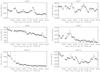 |
Fig. 2 Time series of XBPs (xbp5, xbp7, xbp8, xbp9, xbp10, and xbp14) observed in Ti_poly filter (intensity in DN/s versus start time). |
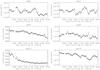 |
Fig. 3 Time series of XBPs (xbp5, xbp7, xbp8, xbp9, xbp10 & xbp14) observed in Al_mesh filter (intensity in DN/s versus start time). |
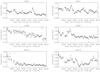 |
Fig. 4 Variation in the intensity ratios (Ti_poly/Al_mesh) of XBPs: xbp5, xbp7, xbp8, xbp9, xbp10, and xbp14 (intensity ratio versus start time). |
Shortly after the launch of Hinode, the contamination from an unknown source began to deposit itself on the XRT CCD at a roughly constant rate. Routine CCD bakeouts do not completely remove this contamination. Although the actual substance(s) are not known, the optical properties, as judged by the change in the filter response to “quiet Sun” plasma, are similar to diethylhexyl phthalate (DEHP). If modelled as DEHP, the contaminant layer at the time of our observations is estimated to be ≈ 1417 Å thick. The effect of the contaminant is highly wavelength dependent, with long wavelengths mostly being absorbed. Consequently, the Al-mesh filter is much more affected than Ti_poly, although the effect in the latter is not negligible. XRT IDL software available in the SSW tree (make_xrt_wave_resp.pro, make_xrt_temp_resp.pro) was used to include this contamination layer in the filter temperature response for our analysis. After including the contamination layer, we derived the filter response curves for both Ti_poly and Al_mesh filters. These curves were used to estimate the temperature of XBPs after determining the intensity ratios. To calculate temperature, Al_mesh images were interpolated to match Ti_poly image scale. Because both images were taken almost simultaneously, no sub-pixel co-alignment of images was performed. A more detailed discussion of the data analysis is also presented along with the results in the following section.
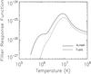 |
Fig. 5 Variations in the XRT Ti_poly & Al_mesh filter responses as a function of temperature after including the contamination layer. |
3. Results and discussion
The temperature fluctuations and morphology of different X-ray bright points and associated plasma properties have not been well understood. Some authors classified the bright points seen at different temperatures as cool and hot components (McIntosh 2007; Tian et al. 2008) in transition region and corona respectively. It will be interesting to know whether there are cooler and hotter bright points (XBPs) at the coronal level.
Our Fig. 1 reveals the different types of XBPs showing different X-ray emission levels with a rich morphology. In the calibrated image, we placed rectangular boxes over the selected XBPs and derived the cumulative intensity values of the XBPs by adding all the pixel intensity values. The light curves of all the XBPs were derived for both the time sequence images. The light curves of 6 XBPs (e.g. xbp5, xbp7, xbp8, xbp9, xbp10 and xbp14) are shown in Fig. 2 for the Ti_poly filter. Similarly in Fig. 3, we present the light curves of these XBPs observed with Al_mesh filter. The intensity oscillation is seen in all the light curves of the XBPs (presented in Figs. 2 and 3) observed with the two filters and the fluctuations have similar patterns in both cases. The temporal variations in the intensity of XBPs observed with Ti_poly filter show an intensity oscillations on timescales of between a few minutes and hours (Kariyappa & Varghese 2008). From Figs. 2 and 3, we note that xbp8 does not exhibit impulsive brightness variations, but that the brightness gradually decreases with time. On the other hand, xbp5, xbp7, xbp9, and xbp14 do show impulsive energy deposition which is presumably caused by reconnection. Some of the variations in brightness shown in Figs. 2 and 3 could be the result of two effects: an actual increase in the surface brightness of XBPs and an increase in the area of XBP. The latter effect can be mitigated by taking the ratio of images observed in two filters. We derived the ratio of the intensity values of each XBP observed with two filters. The variations of the intensity ratios are presented in Fig. 4 for xbp5, xbp7, xbp8, xbp9, xbp10, and xbp14. It is evident from these figures that the fluctuations in the intensity ratio of XBPs are similar to the intensity oscillations shown in Figs. 2 and 3.
To determine the temperature of XBPs, we derived the XRT filter temperature response curves for Ti_poly and Al_mesh after including the contamination layer (see Fig. 5). Using these filter temperature response curves and the intensity ratios, we determined the temperature of each XBP. We estimated the errors in the temperatures by assuming photon statistics for the filter fluxes, and folding these through the filter ratio versus temperature to estimate temperature errors. We stress that these are random errors only; systematic errors due to uncertainties in, e.g., calibrations, the contamination layer, etc. are not included, but are smaller than the random errors. For example, in Fig. 6 we show the temporal variations in temperature of xbp5, xbp7, xbp8, xbp9, xbp10, and xbp14 with error bars (random errors).
All the XBPs exhibit temperature fluctuations similar to intensity oscillations, although the relationship between temperature and intensity oscillations is not linear (see Fig. 7). We note that the temperature is well correlated with the intensity of all the XBPs, except for xbp7 where the temperature is anti-correlated with the intensity. One possible explanation of the anticorrelation for xbp7 could be that the xbp7 is at the end of the reconnection process, when the reconnection between two independent magnetic poles is nearly complete. Figure 3 (right panel) in Longcope & Kankelborg (1999) shows a change in the energy deposit as two poles approach and reconnect with each other. The amount of energy increases, reaches a maximum, and then decreases. Thus, xbp7 is at the late stages of that process, during which the reconnection episodes continue and inject high temperature plasma into corona, although the amount of injected energy is relatively small compared to the energy injected by previous episodes. Hence, there is a large amount of plasma that cools because of radiative cooling; reconnection episodes still produce a variation in brightness, but the high-temperature plasma (supplied by reconnection events) is masked by a bulk of cooler plasma already present above the reconnection site. We found a similar anticorrelation in xbp7 observed with the Al_mesh filter. The above scenario, however, requires verification by means of a detailed study of the evolution of the magnetic properties of XBPs using high-cadence magnetograms. Unfortunately, no such magnetograms of sufficiently high cadence is available for the time period described in this paper.
Mean temperature of XBPs.
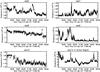 |
Fig. 6 Temperature variations in xbp5, xbp7, xbp8, xbp9, xbp10, and xbp14. The error bars are shown and the mean error in the estimated temperature is about ± 0.01 MK. (temperature in MK versus start time) |
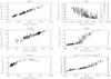 |
Fig. 7 Scatter diagrams of temperature (in MK) versus intensity (in DN/s) measured in Ti_poly of XBPs (xbp5, xbp7, xbp8, xbp9, xbp10, and xbp14). |
We note from Fig. 6 and Table 1 that the average temperature of the 14 XBPs ranges from 1.1 MK to 3.4 MK. The xbp14 is an interesting bright point located in an active region with a higher temperature value of 3.4 MK. This suggests that xbp14 may be heated by a different process from the rest of XBPs. The light curve of xbp14 shows a sharp peak around 19:00–20:00 h where the temperature increases to 7 MK (Fig. 6). This could be due to a nanoflare. However, we have only one such sample in our data set and it would be interesting to make a detailed study of a large sample of active region XBPs to understand the different processes and compare with other XBPs.
McIntosh (2007) classified the bright points seen in He II and soft X-rays as cool and hot bright points, respectively. Similarly, Tian et al. (2008) show that the bright feature seen at coronal temperature represents the hot component, and that the corresponding bright emission at the transition region is the cool component of a bright point. These authors examined the bright point observed at different heights in the solar atmosphere that hence formed at different temperature levels, whereas we found that XBPs of different temperatures are present at the same range of heights in the corona.
The use of filter ratios is only strictly valid for isothermal plasmas, hence it is important to consider just how isothermal XBP plasma is. Brosius et al. (2008), using EUNIS on a sounding rocket, find a differential emission measure (DEM) peak at log T ~ 6.15 and a minimum at log T ~ 5.35 a factor of 3.5 lower in DEM. A similar peak temperature was found earlier by Habbal et al. (1990). Tian et al. (2008) note a two-component structure, one at log T ≈ 6.1−6.3 and one at transition region temperatures log T ≈ 5.2−5.4 (see also McIntosh 2007). XRT is progressively less sensitive to plasma below log T ≈ 6.0 (Fig. 5), and so primarily sees the narrow hot component; Saar et al. (2009) detected a slightly varying ⟨ log T ⟩ in a narrow peak around log T ~ 6.1. Thus, while the DEM may not fall off enormously for log T < 6.0 (Brosius et al. 2008), the drop-off in XRT sensitivity may be sufficient to effectively isolate the hotter XBP DEM peak and ensure that XBPs are effectively isothermal for XRT purposes.
It is interesting to study the relation between the temperature of XBPs (both cooler & hotter) and the strength of the magnetic field, and how the magnetic field plays a role in driving the different brightenings and different temperature values and in the heating mechanisms of the corona at the sites of XBPs. This would require a detailed investigation of high resolution and high-time cadence magnetograms, which were unavailable for a given sequence of XRT observations. Nevertheless, one can gain useful insights from the dynamical evolution and changes in the morphology of XBPs. Our analysis of long time-series observational data taken in multiple filters of the XBPs reveal more of the dynamical nature and the physical properties of different classes (cooler and hotter) of XBPs. XBPs exhibit temperature fluctuations in time (Fig. 6) and the mean temperatures in the range from 1.1 MK to 3.4 MK. We speculate that the temperature fluctuations may be associated with the reconnection of the magnetic field forming XBPs. Comparing Figs. 2, 3, and 6, we see that some XBPs (e.g., xbp8) do not exhibit impulsive variations, but both brightness and temperature gradually decrease with time. This indicates that for xbp8 the reconnection process is complete, and what we see is plasma slowly cooling down. However, the radiative cooling time in the corona should be about 5–20 min (e.g., Aschwanden 2004), so, the reconnection may still take place, but there is no impulsive reconnection. On the other hand, xbp5, xbp7, xbp9, xbp14, and possibly xbp10 do show impulsive energy deposition due to reconnection and the high temperature plasma in these cases is indicative of the reconnection. The temperature values and their variations suggest that the XBPs show a high variability in their temperature and that the heating rate of XBPs is highly variable on short timescales. Verifying the above evolution would require a detailed study of thermal and magnetic properties of XBPs, which we plan to conduct in the near future.
Acknowledgments
Hinode is a Japanese mission developed and launched by ISAS/JAXA, collaborating with NAOJ as a domestic partner, NASA and STFC (UK) as international partners. Scientific operation of the Hinode mission is conducted by the Hinode science team organized at ISAS/JAXA. This team mainly consists of scientists from institutes in the partner countries. Support for the post-launch operation is provided by JAXA and NAOJ (Japan), STFC (UK), NASA (USA), ESA, and NSC (Norway). We are grateful to the Hinode team for all their efforts in the design, build, and operation of the mission. The authors would like to thank Professors Loren Acton and Stuart M. Jefferies for stimulating discussion and valuable suggestions on this research. One of the authors (Kariyappa) wish to express his sincere thanks to Professor Siraj Hasan, Director, Indian Institute of Astrophysics for constant support and encouragement provided during this research work. The National Solar Observatory (NSO) is operated by the Association for Research in Astronomy (AURA, Inc.) under cooperative agreement with the National Science Foundation (NSF). We wish to express our sincere thanks to referee for valuable comments and suggestions that improved the manuscript considerably.
References
- Aschwanden, M. 2004, Physics of the Solar Corona (Springer-Praxis) [Google Scholar]
- Brosius, J. W., Rabin, D. M., Thomas, R. J., & Landi, E. 2008, ApJ, 677, 781 [NASA ADS] [CrossRef] [Google Scholar]
- Cram, L. E., & Damé, L. 1983, ApJ, 272, 355 [NASA ADS] [CrossRef] [Google Scholar]
- Curdt, W., & Heinzel, P. 1998, ApJ, 503, L95 [NASA ADS] [CrossRef] [Google Scholar]
- Golub, L., & Pasachoff, J. M. 1997, The Solar Corona (Cambridge, UK: Cambridge University Press) [Google Scholar]
- Golub, L., Krieger, A. S., Silk, J. K., Timothy, A. F., & Vaiana, G. S. 1974, ApJ, 189, L93 [NASA ADS] [CrossRef] [Google Scholar]
- Golub, L., Krieger, A. S., Harvey, J. W., & Vaiana, G. S. 1977, Sol. Phys., 53, 311 [Google Scholar]
- Golub, L., DeLuca, E., Austin, G., et al. 2007, Sol. Phys., 243, 63 [NASA ADS] [CrossRef] [Google Scholar]
- Habbal, S. R. 1990, in Mechanisms of Chromospheric and Coronal Heating, ed. P. Ulmschneider, E. R. Priest, & R. Rosner (Springer Verlag), 127 [Google Scholar]
- Habbal, S. R., Withbroe, G. L., & Dowdy, J. F. Jr. 1990, ApJ, 352, 333 [Google Scholar]
- Hara, H., & Nakakubo-Morimoto, K. 2003, ApJ, 589, 1062 [NASA ADS] [CrossRef] [Google Scholar]
- Harvey, K. L. 1996, in Magnetic Reconnection in the Solar Atmosphere, ed. R. D. Bentley, & J. T. Mariska, ASP Conf, Ser., 111, 9 [Google Scholar]
- Kankelborg, C. C., & Longcope, D. W. 1999, Sol. Phys., 190, 59 [NASA ADS] [CrossRef] [Google Scholar]
- Karachik, N. V., Pevtsov, A. A., & Sattarov, I. 2006, ApJ, 642, 562 [NASA ADS] [CrossRef] [Google Scholar]
- Kariyappa, R. 1994, Sol. Phys., 154, 19 [NASA ADS] [CrossRef] [Google Scholar]
- Kariyappa, R. 1996, Sol. Phys., 165, 211 [NASA ADS] [CrossRef] [Google Scholar]
- Kariyappa, R. 1999, in 19th NSO/Sac Peak Summer Workshop on High Resolution Solar Physics: Theory, Observations, and Techniques, ASP Conf. Ser., 183, 420 [Google Scholar]
- Kariyappa, R. 2008, A&A., 488, 297 [NASA ADS] [CrossRef] [EDP Sciences] [Google Scholar]
- Kariyappa, R., & Damé, L. 2010, Sol. Phys., submitted [Google Scholar]
- Kariyappa, R., & Pap, J. M. 1996, Sol. Phys., 167, 115 [NASA ADS] [CrossRef] [Google Scholar]
- Kariyappa, R., & Varghese, B. A. 2008, A&A., 485, 289 [NASA ADS] [CrossRef] [EDP Sciences] [Google Scholar]
- Kariyappa, R., Sivaraman, K. R., & Anandaram, M. N. 1994, Sol. Phys., 151, 243 [NASA ADS] [CrossRef] [Google Scholar]
- Kariyappa, R., Varghese, B. A., & Curdt, W. 2001, A&A., 374, 691 [NASA ADS] [CrossRef] [EDP Sciences] [Google Scholar]
- Kariyappa, R., Satyanarayanan, A., & Damé, L. 2005, Bull. Astron. Soc. India, 33, 19 [NASA ADS] [Google Scholar]
- Krieger, A. S., Vaiana, G. S., & Van Speybroeck, L. P. 1971, in Solar Magnetic Fields, ed. R. Howard, IAU Symp., 43, 397 [NASA ADS] [CrossRef] [Google Scholar]
- Longcope, D. W., & Kankelborg, C. C. 1999, ApJ, 524, 483 [NASA ADS] [CrossRef] [Google Scholar]
- Liu, S. Y. 1974, ApJ, 189, 359 [NASA ADS] [CrossRef] [Google Scholar]
- Longcope, D. W., Kankelborg, C. C., Nelson, J. L., & Pevtsov, A. A. 2001, ApJ, 553, 429 [NASA ADS] [CrossRef] [Google Scholar]
- McIntosh, S. W. 2007, ApJ, 670, 1401 [NASA ADS] [CrossRef] [Google Scholar]
- Nakakubo, K., & Hara, H. 1999, Adv. Space Res., 25, 1905 [NASA ADS] [CrossRef] [Google Scholar]
- Saar, S. H., Farid, S., & DeLuca, E. E. 2009, in AIP Conf. Ser. (AIPC), 1094, 756 [Google Scholar]
- Sattarov, I., Pevtsov, A. A., Hojaev, A. S., & Sherdonov, C. T. 2002, ApJ, 564, 1042 [NASA ADS] [CrossRef] [Google Scholar]
- Sattarov, I., Pevtsov, A. A., Karachik, N. V., Sherdanov, C. T., & Tillaboev, A. M. 2010, Sol. Phys., 262, 321 [NASA ADS] [CrossRef] [Google Scholar]
- Strong, K. T., Harvey, K., Hirayama, T., et al. 1992, PASJ, 44, L161 [NASA ADS] [Google Scholar]
- Tian, H., Curdt, W., Marsch, E., & He, J.-S. 2008, ApJ, 681, L121 [Google Scholar]
- Vaiana, G. S., Krieger, A. S., Van Speybroeck, L. P., & Zehnfennig, T. 1970, Bull. Am. Phys. Soc., 15, 611 [Google Scholar]
- Zhang, J., Kundu, M., & White, S. M. 2001, Sol. Phys., 88, 337 [Google Scholar]
All Tables
All Figures
|
Fig. 1 Sample of X-ray images obtained on April 14, 2007 at the center of the solar disk in a quiet region. The field of view for both images is 512′′ × 512′′, the left image being taken with the Ti_poly filter at full resolution (512 × 512 pixels), the right image being taken with the Al_mesh filter binned 2 × 2 (256 × 256 pixels). The analysed XBPs are marked as xbp1, xbp2,..., xbp14. |
| In the text | |
|
Fig. 2 Time series of XBPs (xbp5, xbp7, xbp8, xbp9, xbp10, and xbp14) observed in Ti_poly filter (intensity in DN/s versus start time). |
| In the text | |
|
Fig. 3 Time series of XBPs (xbp5, xbp7, xbp8, xbp9, xbp10 & xbp14) observed in Al_mesh filter (intensity in DN/s versus start time). |
| In the text | |
|
Fig. 4 Variation in the intensity ratios (Ti_poly/Al_mesh) of XBPs: xbp5, xbp7, xbp8, xbp9, xbp10, and xbp14 (intensity ratio versus start time). |
| In the text | |
|
Fig. 5 Variations in the XRT Ti_poly & Al_mesh filter responses as a function of temperature after including the contamination layer. |
| In the text | |
|
Fig. 6 Temperature variations in xbp5, xbp7, xbp8, xbp9, xbp10, and xbp14. The error bars are shown and the mean error in the estimated temperature is about ± 0.01 MK. (temperature in MK versus start time) |
| In the text | |
|
Fig. 7 Scatter diagrams of temperature (in MK) versus intensity (in DN/s) measured in Ti_poly of XBPs (xbp5, xbp7, xbp8, xbp9, xbp10, and xbp14). |
| In the text | |
Current usage metrics show cumulative count of Article Views (full-text article views including HTML views, PDF and ePub downloads, according to the available data) and Abstracts Views on Vision4Press platform.
Data correspond to usage on the plateform after 2015. The current usage metrics is available 48-96 hours after online publication and is updated daily on week days.
Initial download of the metrics may take a while.