| Issue |
A&A
Volume 526, February 2011
|
|
|---|---|---|
| Article Number | A121 | |
| Number of page(s) | 7 | |
| Section | Extragalactic astronomy | |
| DOI | https://doi.org/10.1051/0004-6361/201014168 | |
| Published online | 10 January 2011 | |
Gamma-ray bursts afterglows with energy injection from a spinning down neutron star
1
INAF – Osservatorio Astronomico di Roma, via Frascati 33, Monte Porzio
Catone, Roma,
Italy
2
ASDC, via
Galileo Galilei, 00040
Frascati (Roma),
Italy
⋆⋆
3
INAF – Osservatorio Astronomico di Brera,
via E. Bianchi 46, 23807, Merate (LC), Italy
4
INAF – Istituto di Astrofisica Spaziale e Fisica Cosmica di
Roma, via Fosso del Cavaliere
100, 00133
Roma,
Italy
5
Dipartimento di Astronomia, Universita’ degli Studi di
Bologna, via Ranzani 1,
I 40127
Bologna,
Italy
6
Centre d’Étude Spatiale des Rayonnements, CNRS/UPS,
BP 4346, 31028
Toulouse Cedex 4,
France
Received: 31 January 2010
Accepted: 17 April 2010
Abstract
Aims. We investigate a model for the shallow decay phases of gamma-ray burst (GRB) afterglows discovered by Swift/XRT in the first hours following a GRB event. In the context of the fireball scenario, we consider the possibility that long-lived energy injection from a millisecond spinning, ultramagnetic neutron star (magnetar) powers afterglow emission during this phase.
Methods. We consider the energy evolution in a relativistic shock that is subject to both radiative losses and energy injection from a spinning down magnetar in spherical symmetry. We model the energy injection term through magnetic dipole losses and discuss an approximate treatment for the dynamical evolution of the blastwave. We obtain an analytic solution for the energy evolution in the shock and associated lightcurves. To fully illustrate the potential of our solution we calculate lightcurves for a few selected X-ray afterglows observed by Swift and fit them using our theoretical lightcurves.
Results. Our solution naturally describes in a single picture the properties of the shallow decay phase and the transition to the so-called normal decay phase. In particular, we obtain remarkably good fits to X-ray afterglows for plausible parameters of the magnetar. Even though approximate, our treatment provides a step forward with respect to previously adopted approximations and provides additional support of the idea that a millisecond spinning (1–3 ms), ultramagnetic (B ~ 1014−1015 G) neutron star loosing spin energy through magnetic dipole radiation can explain the luminosity, durations and shapes of X-ray GRB afterglows.
Key words: gamma-ray burst: general / X-rays: bursts / shock waves / stars: magnetars / relativistic processes
Virgo-Ego Scientific Forum fellow.
INAF personnel resident at ASDC.
© ESO, 2011
1. Introduction
Before the launch of Swift in November 2004, X-ray afterglows of long gamma-ray bursts could be pointed at with X-ray telescopes not earlier than several hours after the trigger. These observations showed in most cases a smooth power-law-like decay F(t) ∝ t−α, with typical index of α ≥ 1. With the advent of Swift, X-ray fluxes could be monitored from a few minutes after the burst trigger. These observations have revealed a complex behavior in the first few hours after the GRB, which nonetheless displays remarkably standard properties across different events. This behavior can be described with a double broken power-law, with an initial very steep decay (up to few hundreds of seconds after the trigger) with α > 2 followed by a shallow phase, lasting ~103−104 s, with α < 0.8 and, later on, a steeper “normal” decay with α ~ 1.2−1.4 (Nousek et al. 2006; Gehrels et al. 2009).
The X-ray spectral slope does not change between the shallow and normal decay, in marked contrast to what would be expected if this temporal break was caused by the passage of a characteristic synchrotron frequency in the X-ray band (e.g. Sari et al. 1998). A possible interpretation requiring no spectral variations in the observed energy band invokes prolonged energy injection into the external shock that is believed to give rise to the GRB afterglow. An energy injection could come either from relativistic shells impacting the fireball at late times (e.g. Rees & Meszaros 1998; Sari & Meszaros 2000) or from a long-lived central engine (e.g. Zhang et al. 2006; Nousek et al. 2006; Panaitescu et al. 2006a).
Among different hypotheses about the nature of GRB central engines, two major classes can be identified. The first considers the formation of a black hole-debris torus system, the prompt emission being related to accretion of matter from the torus during the first ~10−100 s (Narayan et al. 1992; Woosley 1993; Meszaros et al. 1999). In this scenario, keeping the energy production active to power the afterglow for at least ~104 s is a difficult and far from settled matter, (Mc Fadyen et al. 2001; Ramirez-Ruiz 2004; Cannizzo & Gehrels 2009; Barkov & Komissarov 2009).
An alternative class of models invokes the formation of a strongly magnetic (B > 1014−1015 G), millisecond spinning neutron star (NS, Usov 1992; Duncan & Thompson 1992; Blackman & Yi 1998; Kluzniak & Ruderman 1998; Wheeler 2000). Recently, time-dependent MHD simulations have shown that long GRBs can originate from the interaction between a relativistic and strongly magnetized wind produced by a newly-born NS and the surrounding stellar envelope. Neutron star spin periods of ~1 ms and ultrastrong magnetic fields, i.e. B ≥ 1015 G, would be required in this case (e.g. Thompson et al. 2004; Bucciantini et al. 2006, 2008, 2009; see also Tchekhovskoy et al. 2009).
The newly formed NS is expected to loose its initial spin energy (>1052 erg) at a very high rate for the first few hours through magnetic-dipole spin down, something that provides a long-lived central engine in a very natural way. Dai & Lu (1998) considered this idea with regard to possible observable effects on the afterglow emission. Zhang & Meszaros (2001) argued that in this scenario, achromatic bumps in afterglow lightcurves are expected for NS spin periods shorter than a few ms and magnetic fields stronger than several times 1014 G. Interestingly, studies of the origin of NS magnetism envisage that the millisecond spin period at birth is the key property that allows a proto-NS to amplify a seed magnetic field to a strength far exceeding 1014 G, through efficient conversion of its initial differential rotation energy (e.g. Duncan & Thompson 1992; Thompson & Duncan 1993). These highly magnetized, fast spinning NSs are expected to loose angular momentum at a high rate in the first decades of their life and later become slowly rotating magnetars, whose major free energy reservoir is in their magnetic field (Thompson & Duncan 1995, 1996, 2001, cf. Woods & Thompson 2006; Mereghetti 2008). We call these NSs magnetars since their birth, although when they spin at a millisecond period, their rotational energy is still the main free energy reservoir.
After the Swift discovery of early afterglow shallow phases, the magnetar scenario has been invoked to interpret the X-ray light curve of both some short and long GRBs (e.g. 051221A by Fan & Xu 2006; 060313 by Yu & Huang 2007; GRB 050801 by De Pasquale et al. 2007; 070110 by Troja et al. 2007). For GRB 060729 this scenario was shown to agree well with the shallow and normal decay phases in the optical and X-ray bands (Grupe et al. 2007; Xu et al. 2009).
Finally we note that besides the interest in understanding GRB physics, the very fast spin and huge magnetic field envisaged in the magnetar formation scenario makes these objects very interesting also for gravitational wave (GW) astronomy. Different possibilities for this to occur have been investigated in the literature (Palomba 2001; Cutler 2002; Stella et al. 2005; Dall’Osso & Stella 2007; Dall’Osso et al. 2009; Corsi & Meszaros 2009) showing that in astrophysically plausible conditions, GW emission might efficiently extract spin energy from the NS, in competition with magnetic dipole losses. The study presented here builds on the ansatz that millisecond spinning magnetars are formed in the events that give rise to long GRBs. We investigate the evolution of energy in a relativistic blastwave subject to radiation losses due to shock deceleration in the ISM and energy injection from a magnetically braking NS. We extend previous treatments by describing the injection term by the standard magnetic dipole formula and deriving a prediction for the evolution of energy and luminosity that can interpret the X-ray afterglows through their shallow and normal decay phases altogether. We derive an approximate solution for the blastwave luminosity, which we compare with X-ray GRB afterglow lightcurves observed by Swift. We obtain a remarkably good match to these lightcurves for the range of initial spin periods and magnetic field strengths expected for magnetars at birth. These results illustrate the potential of this scenario in explaining the early afterglow observations in a simple, unified picture.
2. Relativistic blast wave with energy injection: spherically symmetric case
We assume that a GRB event is associated to the formation of a millisecond spinning, ultramagnetized NS. In the context of the fireball scenario, the energy released in the collapse of the progenitor star produces first a fireball expanding freely at relativistic speed through the ambient medium. The prompt emission is produced at this early stage and is commonly ascribed to internal shocks in the fireball (Rees & Meszaros 1994; Paczynski & Xu 1994; Sari & Piran 1997). A relativistic forward shock is produced at larger distances from the explosion site (~1016 cm), which initially propagates freely through the ambient medium. At a later time, call it td, the mass swept up by the forward shock will be enough to begin affecting the expansion dynamics of the shock itself. This defines the decelaration radius rd ≈ ctd, at which the kinetic energy of the shock starts being efficiently converted to internal energy and then radiation. This corresponds to the onset of the afterglow emission. We focus here only on the deceleration phase, describing the evolution of the total energy within the fireball as matter from the ISM is swept up. Our aim is to interpret the shallow decay phase and subsequent achromatic transition to the “normal” decay phase as observed in X-rays, within a single physical model containing a minimal set of parameters. We do not address here a detailed study of the multiwavelength behaviour of afterglow lightcurves. In Sect. 3.2 we discuss possible developments of our work in this direction, like e.g. a close comparison of model predictions with multiwavelength observations. The first few minutes after the GRB event are characterized by a very steep power-law decay of the flux while a marked spectral change usually accompanies the transition into the shallow decay phase (this is in contrast with the lack of spectral evolution across the shallow-to-normal transition). This initial steep decay is believed to arise from a different spectral component than the X-ray afterglow, likely the tail of the prompt emission (cf. Zhang 2007, for a detailed discussion); we do not consider it in this work.
In addition to the deceleration in the ISM, we study the way in which the afterglow emission is affected by the energy injection caused by the spindown of the newly formed magnetar. We first introduce time t as that measured by a clock at rest in the NS (central engine) frame. In this frame the NS loses rotational energy, likely in the form of a strongly magnetised particle wind, with a luminosity Lsd(t) according to the usual magnetic dipole spindown formula 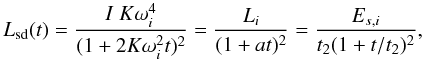 (1)where I is the NS moment of inertia, K = B2R6/(6Ic3) with B the (dipole) magnetic field at the NS pole, R the NS radius and c the speed of light. In the second equality, the quantity Li = Lsd(ti) represents the spindown luminosity at the initial time (ti) when spindown through magnetic dipole radiation sets in, and
  , where t2 represents the spindown timescale at time ti and ωi is the initial spin frequency. Es,i is the NS spin energy at time ti, so that Li = Es,i/t2. The energy carried by the wind travels essentially at the speed of light, so that the energy emitted at later times by the NS can be transferred to the shock.
To calculate the expected behaviour of the lightcurve we start from the energy balance of the relativistic blastwave subject to the energy injection in Eq. (1) along with radiative losses. The latter are described by following the prescription of Cohen et al. (1998). For the time being we assume spherical symmetry of all processes involved, which allows us to write the complete energy equation of the blast wave as ![Mathematical equation: \begin{equation} \label{energyone} \frac{{\rm d}E}{{\rm d}t} = L_{\rm inj}(t) - k\frac{E}{t} = (1-\beta) L_{\rm sd}\left[t-\frac{r(t)}{c}\right] - k \frac{E}{t}\cdot \end{equation}](/articles/aa/full_html/2011/02/aa14168-10/aa14168-10-eq37.png) (2)Here k = 4ϵe, with ϵe the fraction of the total energy that is transferred to the electrons, r(t) is the radius of the blast wave at time t and all quantities are expressed in the frame of the central engine. Note that Linj represents the rate at which energy is injected in the shock at time t. This quantity is related to the rate at which the central NS emitted energy – Lsd – at a previous time, t − r(t)/c. In the central engine rest frame, an infinitesimal time interval dt is related to the infinitesimal displacement of the blast wave dr = cβ(t)dt. However, due to propagation effects, photons emitted at two successive radii will be received by the observer over a much shorter time interval dT, which defines what is called “the observer’s time” (T). The relation between dt and dT is1
(2)Here k = 4ϵe, with ϵe the fraction of the total energy that is transferred to the electrons, r(t) is the radius of the blast wave at time t and all quantities are expressed in the frame of the central engine. Note that Linj represents the rate at which energy is injected in the shock at time t. This quantity is related to the rate at which the central NS emitted energy – Lsd – at a previous time, t − r(t)/c. In the central engine rest frame, an infinitesimal time interval dt is related to the infinitesimal displacement of the blast wave dr = cβ(t)dt. However, due to propagation effects, photons emitted at two successive radii will be received by the observer over a much shorter time interval dT, which defines what is called “the observer’s time” (T). The relation between dt and dT is1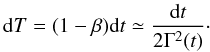 (3)When integrated, this gives T = t − r(t)/c. Now we can transform Eq. (2) to the equivalent form with respect to time T, using Eq. (3). After some manipulation one obtains
 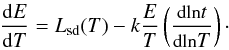 (4)In order to obtain t(T), Γ(t) is required (see Eq. (3)); this in turn requires a study of the hydrodynamical evolution of the blast wave. The solution to this problem with energy injection is far from trivial and beyond the scope of the present paper. Here we introduce an approximation to derive a solution to the problem which captures all the essential physics. Customarily the evolution of Γ in the deceleration phase is treated using self-similar solutions for relativistic blastwaves (Blandford & McKee 1976; Piran 1999). In this case all quantities scale as power-laws (with time t). Upon writing Γ2 ∝ t−m one can solve Eq. (3) and obtain T = t/ [2(m + 1)Γ2] , from which dlnt/dlnT = 1/(1 + m) can be substituted in Eq. (4) to obtain E(T). On the other hand, in the problem we are considering the shock evolution is not self-similar because the energy injection term introduces in the problem the timescale t2 = a-1. One can evaluate the change introduced by this complication with an integral expression for the total (internal plus kinetic) energy of the shock (Zhang & Meszaros 2001)
 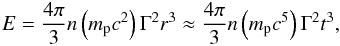 (5)where r ≈ ct has been assumed. By neglecting for the sake of simplicity radial variations in the density of the ambient medium, we can thus write Γ as a function of the shock energy and time t, namely Γ2 ∝ E/t3. For self-similar solutions one obtains E ∝ t3−m; adiabatic shocks thus correspond to m = 3. The relation between Γ and E expressed by Eq. (5) identifies two extremes for the evolution of Γ. First, neglecting radiative losses correponds to the fastest possible growth rate for E which, in turn, corresponds to the slowest decay rate for Γ2. On the other hand, neglecting energy injection corresponds to the fastest possible decay rate for E and, in turn, of Γ2. Any realistic behaviour of Γ is thus expected to lie between these two extremes.
In the former case, which is appropriate for the early stages of energy injection, we can write to a very good approximation  (6)The solution to this gives E ∝ t2 and, thus, Γ2 ∝ t-1 or dlnt/dlnT = 1/2. In the opposite extreme, where only radiation losses are present, one obtains E ∝ t−k which implies Γ2 ∝ t−(3 + k) (with, in general, k < 1) or dlnt/dlnT = 1/(4 + k). Note that these extremes reproduce, as expected, the self-similar solution obtained by Zhang & Meszaros (2001).
Hence, although the coefficient multiplying E/T in Eq. (4) does depend on time, its value will be bracketed between the two extremes found above2, as long as E ∝ Γ2t3 holds. As these extremes differ by a factor 2 + k/2 at most, we can consider dlnt/dlnT ≈ const. as a reasonable first-order approximation, neglecting the slow and moderate change of dlnt/dlnT. This allows us to write the energy equation as  (7)where k′ = k(dlnt/dlnT) ≈ const. Note that its value will also depend on the unknown density profile of the ambient medium, about which we do not make any assumptions. Our ignorance about it is completely contained in the free parameter k′, as is our ignorance about the microphysics. In general, fixing all other parameters, we expect higher values of k′ for a wind-like medium than for a constant density ISM, based on the discussion above. As far as our present work is concerned, the solution to Eq. (7) can be cast in the form
  (8)where T0 ≥ Td is any time chosen as the initial condition. The integral in the above expression can be expressed in terms of the (real valued) hypergeometric function
 (9)where z = (1 + aT)-1. Inserting this expression in the above Eq. (8), we obtain the complete functional form of E(T) and can accordingly re-express the energy loss term of Eq. (4) as L(T) = k′E(T)/T, which represents the total (bolometric) luminosity of the blastwave. The resulting function thus provides the total bolometric luminosity as a function of (observer’s) time T. Below we use it as an approximation to the X-ray lightcurve to compare it with the X-ray data. This assumes that the observed X-ray luminosity matches the bolometric luminosity, a reasonable approximation as long as the X-ray flux is the dominant emission component, which is mainly true in the early stages of the afterglow.
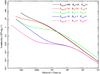 |
Fig. 1 Five different theoretical (bolometric) lightcurves from the model presented here, drawn varying the initial energy of the afterglow (Eimp), the dipole magnetic field (B) and the initial spin period (Pi,ms) of the NS. All lightcurves are obtained for the same value of k′ = 0.4. The time at which each lightcurve begins is the deceleration time Td, estimated for illustration purposes simply by equating the initial energy Eimp to the rest-mass energy of swept up matter in a constant density ISM (n ≃ 1 cm-3). |
3. Discussion
In order to illustrate the salient properties of our solution, we plot in Fig. 1 five lightcurves calculated through Eqs. (8) and (9). These correspond to a choice of typical values for the shock initial energy, spin period and (dipole) magnetic field of the newly formed magnetar. For all curves a value k′ = 0.4 for the radiative efficiency was assumed.
The curves in Fig. (1) highlight some general features of the solution, which are not related to the nature of our approximation. In general, the model predictions depend mainly on three key parameters: the NS initial spin energy, its (dipole) external magnetic field and the initial energy in the blast wave. The observed X-ray lightcurves of GRB afterglows display a range of shapes, normalizations and durations which our model can account for in a very natural way. On average, the shallow phase is not flat but characterized by a negative slope, smoothly steepening over time as energy injection decreases and radiative losses become more important. Indeed, the NS spindown luminosity itself, i.e. the energy injection term, has an effective power-law slope αsd (to distinguish it from α of the observed afterglow lightcurve), which is expressed as αsd(t) = −2(t/t2)/(1 + t/t2). This equals zero at t = 0 and gradually steepens with time, reaching the value αsd = 1 at t = t2 and, eventually, αsd → 2 for t → ∞. This allows a simple understanding of the lightcurve shapes and their dependence on the parameters.
Given the form of the radiative loss term, ~E/T, the condition dE/dT > 0 is necessary and sufficient for the shallow decay phase to occur, namely a part of the lightcurve where the temporal index of the power-law decay is smaller than 1. Therefore, the onset of the shallow decay phase can be defined by the requirement Linj(T) > kE(T)/T. This leads to a bound on the time at which the shallow phase starts, which can be expressed in terms of the ratio x = T/T2 as 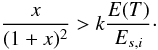 (10)In general, at the initial stage of afterglow emission, the high value of E and low value of T make it likely that radiative losses dominate over the injection term. Starting from the initial (kinetic) energy of the explosion, E0, the afterglow luminosity will then decay as a power-law with index (1 + k). In this situation, one has E(T) = E0(T0/T)k which inserted in Eq. (10) above gives
 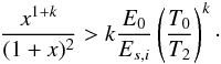 (11)Inserting T = T0(≪T2) into this equation, and then defining x0 = T0/T2, one sees that the shallow phase can start right at time T0 if x0/(1 + x0)2 > kE0/Es,i. However, because the left hand side in this inequality is ≪1 by definition, the condition could be verified only for a very low ratio E0/Es,i. Although this might happen in some cases, one does not expect this to be a general occurrence, so that an initial power-law decay of the lightcurve, with an index α = 1 + k > 1 is to be expected in general. After some time, however, condition (11) will be met so that the energy injection will overcome radiative losses, the total energy within the shell will start increasing over time and the lightcurve will flatten accordingly.
This shallow decay phase will clearly last as long as the energy injection is sufficiently strong to balance radiative losses, a condition that is bound to fail somewhere after time T2. Indeed, we know that during the shallow phase E(T) increases over time ∝ Tβ, with β < 1 and, as long as T < T2, x on the left-hand side of Eq. (10) grows ~T. Hence, if that inequality was satisfied at some early time, it will continue to hold at least up to ~T2. After time T2, on the other hand, both the left-hand side and right-hand side of Eq. (10) start decreasing with an increasing dependence on time. However, while the latter term has an asymptotic decay ∝ T−k dictated by the form of radiative losses, the former term has a steeper asymptotic decay, ∝ T-1, dictated by the form of the injection term. Therefore the inequality expressed in Eq. (10) is bound to reverse sign at some time T > T2, which implies dE/dT < 0 at that time and the afterglow luminosity will eventually decay again ∝ T−(1 + k).
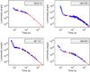 |
Fig. 2 Least-square fit to the X-ray lightcurves of four selected GRB afterglows observed by Swift/XRT obtained through our Eqs. (8) and (9). The blue points and red lines represent the measured (isotropic) luminosity (in the 0.3–100 keV energy range) and best fits, respectively. The starting time T0 was determined for each afterglow based on the end of the spectral transition from the previous steep-decay phase, as discussed in the text. Best-fit parameter values for each individual lightcurve are reported in Table 1. |
A natural anticorrelation between the duration of the shallow phase and its luminosity, i.e. the afterglow luminosity, is also apparent from our model lightcurves, again matching one of the salient properties of observed X-ray afterglows (Sato et al. 2007; Dainotti et al. 2008). In the light of the above discussion it is straightforward to see that this anticorrelation reflects an intrinsic property of the energy injection model assumed, i.e. of magnetic dipole spindown. Indeed, NSs with a higher spindown luminosity will have a shorter spindown timescale on average. This can be checked from the last step in Eq. (1), in the limit t < t2 appropriate for the shallow decay phase, showing that the NS initial spindown luminosity is  , while
  .
.
This point also leads to the expectation that the most luminous among all GRBs/afterglows might even lack a shallow phase altogether. This expectation can also be seen directly from Eq. (11). The left-hand side of that equation has indeed a maximum at x = (1 + k)/(1 − k) which means that if the right-hand side were always greater than that maximum, the condition dE/dT > 0 could never be met. As an example, choosing k = 0.5 gives a maximum ≃ 0.325 at x = 3. Therefore, no shallow decay phase would occur if E0/Es,i > 0.65(T2/T0)1/2. From this example we see that for a given initial spin energy, lower values of T2 (implying stronger magnetic fields) can more easily lead to a lack of the shallow decay phase. On the other hand, for a given T2, lower values of the initial spin energy (again implying higher values of the magnetic field) favour the lack of a shallow phase.
Finally we note that even starting with largely different initial luminosities, theoretical lightcurves converge to a narrow distribution in luminosity at late times, nicely reproducing a property of observed lightcurves (cf. Nousek et al. 2006, their Fig. 2). Again, this can be easily understood in terms of the above discussion. All lightcurves evolve as T−(1+k) at late times, i.e. for t ≫ t2 when energy injection has long ceased, so that they are all parallel for a fixed value of k′. Second, the general anticorrelation between luminosity and duration of energy injection implies that lower luminosity plateaus will in general last longer than higher luminosity ones. Therefore the power-law decay starts earlier in more luminous afterglows, while less luminous ones are still (nearly) flat, which naturally causes all late power-law segments to look as if they had very similar normalizations. Basically, this will reflect the overall energy budget of the blastwave, including both the initial kinetic energy and the energy injected in the later phase. Note that if the same total energy is injected over a longer time – hence, at a lower luminosity – it can produce a late power-law decay with a slightly higher normalization, as is clear from the second and third curves in Fig. 1.
3.1. Comparison with observations and results
In order to further assess the goodness of our treatment, we show in Fig. (2) fits to four selected X-ray afterglows observed by Swift, based on our solution (see Eq. (8)). The afterglows were chosen for illustration purposes among GRBs with known redshifts, good statistics in the XRT lightcurves, clear evidence for a shallow phase, sufficiently long monitoring (>105 s after the trigger) and absence of bright flares or re-brightenings superposed on their lightcurves.
To approximate bolometric luminosity, we obtained rest frame 0.3–100 keV light curves (Fig. 2) from the observed 0.3–10 keV counts rate (taken from Swift XRT lightcurve repository, see Evans et al. 2006, 2009), assuming an absorbed power-law spectral model over the shallow phase, including also the subsequent normal decay if necessary. The resulting (isotropic) luminosities were calculated by multiplying the fluxes by  , with DL the luminosity distance calculated by assuming a standard ΛCDM cosmology with Ωm = 0.27, ΩΛ = 0.73 and H0 = 0.73 km s-1 Mpc-1. Finally, the observer’s times were corrected for the redshift of the source. In accordance with the idea that the initial steep decay phase results from the prompt event, we only fitted data points from the onset of the shallow decay phase, as determined by the time at which the spectral transition of the X-ray emission takes place (our T0).
We note that even though only data points for T > T0 ~ 100 s were fitted, the initial spin energy of our model refers to the time at which magnetic dipole braking sets in, which, in general, is earlier than T0. Moreover, the magnetic field is assumed to remain constant. We stress that our derived values of the radiative efficiency k′ should be taken with some caution. As discussed in the previous section, the degeneracy between the different parameters that determine k′ can only be solved through detailed hydrodynamical models and joint multiwavelength fits to observations. Here we note that best-fit values of k′ correspond to values of ϵe in a relatively wide and fully acceptable range between 0.1 and 0.8, depending on the exact relation between t and T. The results of our fits show that our model agrees with the data in our sample. Neutron star parameters resulting from our least-squares fits are reported in Table 1. We stress that the initial spin periods, ~1−3 ms, and the magnetic fields, several times 1014 G up to slightly larger than 1015 G, perfectly match the parameter range expected for newly born, millisecond spinning magnetars, if their seed magnetic fields were amplified to ultrastrong values by a strong α − Ω dynamo in the first seconds after formation (Duncan & Thompson 1992). In addition, we note that the derived magnetic field values also perfectly match the values of the dipole fields measured in galactic X-ray sources thought to host magnetars, namely the anomalous X-ray pulsars and soft gamma-ray repeaters (see Woods & Thompson 2006; Mereghetti 2008). Finally, the required initial spin periods imply spin energies in the range (3 × 1051−3 × 1052) erg, for a NS moment of inertia I ≃ 1.4 × 1045 g cm2 (cf. Lattimer & Prakash 2001). Note that this is a very conservative estimate of the total spin energy of the NS at formation, because we are only measuring the spin energy of the NS as magnetic dipole losses set in as the dominant spindown mechanism. Additional mechanisms have been proposed, which might be initially more efficient in extracting the NS spin energy and angular momentum, as long as it spins at ≃ 1 ms (cf. Bucciantini et al. 2006, 2008; Dall’Osso et al. 2009; Metzger 2010).
Best-Fit parameters for the four selected GRBs.
We finally note that in at least one case (GRB060729), the X-ray luminosity at late times is somewhat lower than the model prediction. This can be caused by effects that were not considered in our simple model, of which we breifly mention two. First, as we discussed in Sect. 2, forcing the model to fit the whole lightcurve with a fixed value of dlnt/dlnT can lead to an overestimate (by a factor of 2 at most) of the late time emission for a given shallow phase luminosity. This is just of the correct magnitude to explain the mismatch in the case of GRB060729.
Secondly, fitting the X-ray lightcurves with the bolometric luminosity can lead to an overestimate, particularly at late times. Indeed the X-ray lightcurves probably are not representative of the bolometric luminosity at late times, when the contribution of other, lower frequency bands to the total emission becomes non-negligible.
3.2. Further developments
We briefly mention here some of the points that deserve futher comment and which we identify as the most important steps to improve the model beyond the present treatment.
As found by several authors (Panaitescu et al. 2006b; Liang et al. 2007), the optical lightcurves of several GRB afterglows show a chromatic behaviour when compared to X-ray lightcurves, namely they do not show any break at the shallow-to-normal break observed in X-rays. According to Liang et al. (2007), about half of the GRB afterglows with simultaneous X-ray and optical observations show this chromatic behaviour. This is customarily viewed as a major problem for most models invoked to explain the shallow decay phase, at least for half the afterglows. As far as the model introduced here is concerned, a self-consistent solution of Γ(t) is required for a detailed calculation of the expected synchrotron emission at different frequencies (cf. Zhang & Meszaros 2004; Sari 2006). This will permit to derive multiband lightcurves up to late times, which can be compared with multiwavelenght observations of GRB afterglows. However we stress here that a different behaviour of the optical and X-ray lightcurves is to be expected in general in the synchrotron emission from the external shock, if a spectral break frequency were located between the X-ray and optical bands (as already noted by Panaitescu et al. 2006b). This is a natural property of a flow in the slow-cooling regime, if the cooling frequency lies above the optical band but below the X-ray band during (most of) the energy injection phase. In this case, while electrons contributing to the X-ray emission are re-radiating instantaneously all the energy that is transferred to them, electrons emitting in the optical are radiating only a tiny fraction of it. Therefore, the optical emission can evolve indipendently of the injection term for a while, until the emitting electrons nearly exhaust the energy that they accumulated. We will present a quantitative treatment of this issue in a future paper. The assumed geometry of the expanding ejecta also deserves some discussion. Although the subject is still open to debate, there exists by now considerable evidence that GRB fireballs are beamed, likely with opening angles of several degrees (Frail et al. 2001; Ghirlanda et al. 2004; Nava et al. 2007; Liang et al. 2008; Racusin et al. 2009; Cenko et al. 2009). It is important to realize that the energetic requirements of the central engine as derived from our fits are not sensitive to the degree of beaming of the ejecta. This is true as long as the NS emits its spindown luminosity in a nearly isotropic way, as envisaged in models of NS magnetospheres loosing spin energy and angular momentum through the open field lines (Contopoulos et al. 1999; Gruzinov 2005; Spitkovsky 2006). In this case, only a fraction ~ of the rotational energy losses will be transferred to the ejecta and contribute to Linj in Eq. (2), where θj is the opening angle of the beam. On the other hand, the measured luminosity of the afterglow would have to be decreased by the same factor, thus leaving the inferred (isotropic) spindown luminosity of the NS unaffected. The characteristic timescale t2 of energy injection is also unaffected by beaming, implying that our derived values of the dipole magnetic field are also independent of beaming in this case.
On the contrary, if the millisecond spinning NS were to emit its spindown luminosity in a beam of comparable size to the beam of the fireball, then all its power would be transferred to the ejecta. The required spin energy of the NS (∝  ) would have to be reduced accordingly by a factor ~
 . In this case, since the timescale
  is always independent of beaming, our derived values of the magnetic field would have to be increased by a factor ~
 .
.
4. Conclusions
In the framework of prolonged energy injection models for GRB afterglows observed by Swift, we have considered the possibility that newly born magnetars – strongly magnetized and millisecond spinning NSs – are formed in the events producing (long) GRBs. In the first hours after formation of the NSs, the high spindown luminosity caused by magnetic dipole radiation losses represents a natural mechanism for prolonged energy injection in the external shock. To assess the viability of this scenario we considered the energy balance of a blastwave subject to injection of energy by a NS spinning down through magnetic dipole radiation, along with radiative losses (∝ E/t). We found an approximate expression for the (isotropic) bolometric luminosity of the blastwave as a function of time that substantially agrees with the general properties of the shallow-decay and normal-decay phases of X-ray GRB afterglows observed by Swift.
Moreover, we have shown that individual lightcurves can be very well fitted by our derived expression for the bolometric luminosity of the continuously-powered blastwave. In particular, our best fits provide values for the initial spin period of the NS in the range 1–3 ms, which match well the values expected in magnetar formation scenarios. Best-fit values for the magnetic dipole field, 1014−1015 G, are also in the range expected for these objects at formation and agree with the dipole fields estimated for anomalous X-ray pulsars and soft gamma-ray repeaters, the candidate magnetars in our Galaxy.
The second equality holds since β ≃ 1.
Note that for a wind-like medium whose density declines as r-2, similar conclusions would hold: adiabatic shocks correspond to m = 1, while dlnt/dlnT = 1 and 1/(1 + k) for the two extremes, respectively.
Acknowledgments
This work made use of data supplied by the UK Swift Science Data Centre at the University of Leicester. S.D. acknowledges support from a VESF Fellowship. S.D. thanks Prof. S. N. Shore for insightful discussions and helpful comments.
References
- Barkov, M. V., & Komissarov, S. S. 2009, MNRAS, 1713 [Google Scholar]
- Bianco, C. L., & Ruffini, R. 2004, ApJ, 605, L1 [NASA ADS] [CrossRef] [Google Scholar]
- Blackman, E. G., & Yi, I. 1998, ApJ, 498, L31 [Google Scholar]
- Blandford, R. D., & McKee, C. F. 1976, Phys. Fluids, 19, 1130 [NASA ADS] [CrossRef] [Google Scholar]
- Bucciantini, N., Thompson, T. A., Arons, J., Quataert, E., & Del Zanna, L. 2006, MNRAS, 368, 1717 [NASA ADS] [CrossRef] [Google Scholar]
- Bucciantini, N., Quataert, E., Arons, J., Metzger, B. D., & Thompson, T. A. 2008, MNRAS, 383, L25 [NASA ADS] [Google Scholar]
- Bucciantini, N., Quataert, E., Metzger, B. D., et al. 2009, MNRAS, 396, 2038 [NASA ADS] [CrossRef] [Google Scholar]
- Cannizzo, J. K., & Gehrels, N. 2009, ApJ, 700, 1047 [NASA ADS] [CrossRef] [Google Scholar]
- Cenko, S. B., Frail, D. A., Harrison, F. A., et al. 2010, ApJ, 711, 641 [NASA ADS] [CrossRef] [Google Scholar]
- Cohen, E., Piran, T., & Sari, R. 1998, ApJ, 509, 717 [NASA ADS] [CrossRef] [Google Scholar]
- Contopoulos, I., Kazanas, D., & Fendt, C. 1999, ApJ, 511, 351 [Google Scholar]
- Corsi, A., & Mészáros, P. 2009, ApJ, 702, 1171 [NASA ADS] [CrossRef] [Google Scholar]
- Cutler, C. 2002, Phys. Rev. D, 66, 084025 [NASA ADS] [CrossRef] [Google Scholar]
- Dai, Z. G., & Lu, T. 1998, A&A, 333, L87 [NASA ADS] [Google Scholar]
- Dainotti, M. G., Cardone, V. F., & Capozziello, S. 2008, MNRAS, 391, L79 [NASA ADS] [CrossRef] [Google Scholar]
- Dall’Osso, S., & Stella, L. 2007, Ap&SS, 308, 119 [NASA ADS] [CrossRef] [Google Scholar]
- Dall’Osso, S., Shore, S. N., & Stella, L. 2009, MNRAS, 398, 1869 [NASA ADS] [CrossRef] [Google Scholar]
- de Pasquale, M., Oates, S. R., Page, M. J., et al. 2007, MNRAS, 377, 1638 [NASA ADS] [CrossRef] [Google Scholar]
- Duncan, R. C., & Thompson, C. 1992, ApJ, 392, L9 [NASA ADS] [CrossRef] [Google Scholar]
- Evans, P. A., Beardmore, A. P., Page, K. L., et al. 2007, A&A, 469, 379 [NASA ADS] [CrossRef] [EDP Sciences] [Google Scholar]
- Evans, P. A., Beardmore, A. P., Page, K. L., et al. 2009, MNRAS, 397, 1177 [NASA ADS] [CrossRef] [Google Scholar]
- Fan, Y.-Z., & Xu, D. 2006, MNRAS, 372, L19 [NASA ADS] [CrossRef] [Google Scholar]
- Frail, D. A., Kulkarni, S. R., Sari, R., et al. 2001, ApJ, 562, L55 [NASA ADS] [CrossRef] [Google Scholar]
- Gehrels, N., Ramirez-Ruiz, E., & Fox, D. B. 2009, ARA&A, 47, 567 [NASA ADS] [CrossRef] [Google Scholar]
- Ghirlanda, G., Ghisellini, G., Lazzati, D., & Firmani, C. 2004, ApJ, 613, L13 [NASA ADS] [CrossRef] [Google Scholar]
- Grupe, D., Gronwall, C., Wang, X.-Y., et al. 2007, ApJ, 662, 443 [NASA ADS] [CrossRef] [Google Scholar]
- Gruzinov, A. 2005, Phys. Rev. Lett., 94, 021101 [NASA ADS] [CrossRef] [PubMed] [Google Scholar]
- Kluźniak, W., & Ruderman, M. 1998, ApJ, 505, L113 [NASA ADS] [CrossRef] [Google Scholar]
- Liang, E.-W., Zhang, B.-B., & Zhang, B. 2007, ApJ, 670, 565 [NASA ADS] [CrossRef] [Google Scholar]
- Liang, E.-W., Racusin, J. L., Zhang, B., Zhang, B.-B., & Burrows, D. N. 2008, ApJ, 675, 528 [NASA ADS] [CrossRef] [Google Scholar]
- Lyons, N., O’Brien, P. T., Zhang, B., et al. 2010, MNRAS, 402, L705 [NASA ADS] [CrossRef] [Google Scholar]
- MacFadyen, A. I., Woosley, S. E., & Heger, A. 2001, ApJ, 550, 410 [NASA ADS] [CrossRef] [Google Scholar]
- Mereghetti, S. 2008, A&A Rev., 15, 225 [NASA ADS] [CrossRef] [Google Scholar]
- Meszaros, P., Rees, M. J., & Wijers, R. A. M. J. 1999, New Astron., 4, 303 [NASA ADS] [CrossRef] [Google Scholar]
- Metzger, B. D. 2010, in of the Frank N. Bash Symposium 2009 New Horizons in Astronomy, ed. L. Stanford, L. Hao, Y. Mao, & J. Green, ASP Conf. Proc. [arXiv:1001.5046] [Google Scholar]
- Narayan, R., Paczynski, B., & Piran, T. 1992, ApJ, 395, L83 [NASA ADS] [CrossRef] [Google Scholar]
- Nava, L., Ghisellini, G., Ghirlanda, G., et al. 2007, MNRAS, 377, 1464 [NASA ADS] [CrossRef] [Google Scholar]
- Palomba, C. 2001, A&A, 367, 525 [NASA ADS] [CrossRef] [EDP Sciences] [Google Scholar]
- Paczynski, B., & Xu, G. 1994, ApJ, 427, 708 [NASA ADS] [CrossRef] [Google Scholar]
- Panaitescu, A., Mészáros, P., Gehrels, N., Burrows, D., & Nousek, J. 2006a, MNRAS, 366, 1357 [NASA ADS] [CrossRef] [Google Scholar]
- Panaitescu, A., Mészáros, P., Burrows, D., et al. 2006b, MNRAS, 369, 2059 [NASA ADS] [CrossRef] [Google Scholar]
- Piran, T. 1999, Phys. Rep., 314, 575 [Google Scholar]
- Racusin, J. L., Liang, E. W., Burrows, D. N., et al. 2009, ApJ, 698, 43 [NASA ADS] [CrossRef] [Google Scholar]
- Ramirez-Ruiz, E. 2004, MNRAS, 349, L38 [NASA ADS] [CrossRef] [Google Scholar]
- Rees, M. J., & Meszaros, P. 1994, ApJ, 430, L93 [NASA ADS] [CrossRef] [Google Scholar]
- Rees, M. J., & Meszaros, P. 1998, ApJ, 496, L1 [NASA ADS] [CrossRef] [Google Scholar]
- Sari, R., & Piran, T. 1997, MNRAS, 287, 110 [NASA ADS] [CrossRef] [Google Scholar]
- Sari, R., Piran, T., & Narayan, R. 1998, ApJ, 497, L17 [NASA ADS] [CrossRef] [Google Scholar]
- Sari, R., & Mészáros, P. 2000, ApJ, 535, L33 [NASA ADS] [CrossRef] [PubMed] [Google Scholar]
- Sari, R. 2006, Relativistic Jets: The Common Physics of AGN, Microquasars, and Gamma-Ray Bursts, 856, 33 [Google Scholar]
- Sato, R., Ioka, K., Toma, K., et al. 2007, unpublished [arXiv:0711.0903] [Google Scholar]
- Spitkovsky, A. 2006, ApJ, 648, L51 [NASA ADS] [CrossRef] [Google Scholar]
- Stella, L., Dall’Osso, S., Israel, G. L., & Vecchio, A. 2005, ApJ, 634, L165 [NASA ADS] [CrossRef] [Google Scholar]
- Taub, A. H. 1948, Phys. Rev. , 74, 328 [NASA ADS] [CrossRef] [Google Scholar]
- Tchekhovskoy, A., McKinney, J. C., & Narayan, R. 2009, ApJ, 699, 1789 [NASA ADS] [CrossRef] [Google Scholar]
- Thompson, C., & Duncan, R. C. 1993, ApJ, 408, 194 [NASA ADS] [CrossRef] [Google Scholar]
- Thompson, C., & Duncan, R. C. 1995, MNRAS, 275, 255 [NASA ADS] [CrossRef] [Google Scholar]
- Thompson, C., & Duncan, R. C. 1996, ApJ, 473, 322 [NASA ADS] [CrossRef] [Google Scholar]
- Thompson, C., & Duncan, R. C. 2001, ApJ, 561, 980 [NASA ADS] [CrossRef] [Google Scholar]
- Thompson, T. A., Chang, P., & Quataert, E. 2004, ApJ, 611, 380 [NASA ADS] [CrossRef] [Google Scholar]
- Troja, E., Cusumano, G., O’Brien, P. T., et al. 2007, ApJ, 665, 599 [NASA ADS] [CrossRef] [Google Scholar]
- Usov, V. V. 1992, Nature, 357, 472 [NASA ADS] [CrossRef] [Google Scholar]
- Wheeler, J. C., Yi, I., Höflich, P., & Wang, L. 2000, ApJ, 537, 810 [NASA ADS] [CrossRef] [Google Scholar]
- Woods, P. M., & Thompson, C. 2006, Soft gamma repeaters and anomalous X-ray pulsars: magnetar candidates, Compact stellar X-ray sources, 547, ed. W. H. G. Lewin, & M. van der Klis [Google Scholar]
- Woosley, S. E. 1993, ApJ, 405, 273 [NASA ADS] [CrossRef] [Google Scholar]
- Ming, Xu, Yong-Feng, Huang, & Tan, Lu 2009, Res. Astron. Astrophys., 9, 1317 [NASA ADS] [CrossRef] [Google Scholar]
- Yu, Y., & Huang, Y.-F. 2007, Chinese J. Astron. Astrophys., 7, 669 [NASA ADS] [CrossRef] [Google Scholar]
- Zhang, B. 2007, Chinese J. Astron. Astrophys., 7, 1 [Google Scholar]
- Zhang, B., & Mészáros, P. 2001, ApJ, 552, L35 [NASA ADS] [CrossRef] [Google Scholar]
- Zhang, B., & Mészáros, P. 2004, Int. J. Mod. Phys. A, 19, 2385 [NASA ADS] [CrossRef] [Google Scholar]
- Zhang, B., Fan, Y. Z., Dyks, J., et al. 2006, ApJ, 642, 354 [NASA ADS] [CrossRef] [Google Scholar]
All Tables
All Figures
|
Fig. 1 Five different theoretical (bolometric) lightcurves from the model presented here, drawn varying the initial energy of the afterglow (Eimp), the dipole magnetic field (B) and the initial spin period (Pi,ms) of the NS. All lightcurves are obtained for the same value of k′ = 0.4. The time at which each lightcurve begins is the deceleration time Td, estimated for illustration purposes simply by equating the initial energy Eimp to the rest-mass energy of swept up matter in a constant density ISM (n ≃ 1 cm-3). |
| In the text | |
|
Fig. 2 Least-square fit to the X-ray lightcurves of four selected GRB afterglows observed by Swift/XRT obtained through our Eqs. (8) and (9). The blue points and red lines represent the measured (isotropic) luminosity (in the 0.3–100 keV energy range) and best fits, respectively. The starting time T0 was determined for each afterglow based on the end of the spectral transition from the previous steep-decay phase, as discussed in the text. Best-fit parameter values for each individual lightcurve are reported in Table 1. |
| In the text | |
Current usage metrics show cumulative count of Article Views (full-text article views including HTML views, PDF and ePub downloads, according to the available data) and Abstracts Views on Vision4Press platform.
Data correspond to usage on the plateform after 2015. The current usage metrics is available 48-96 hours after online publication and is updated daily on week days.
Initial download of the metrics may take a while.