| Issue |
A&A
Volume 526, February 2011
|
|
|---|---|---|
| Article Number | A154 | |
| Number of page(s) | 6 | |
| Section | Extragalactic astronomy | |
| DOI | https://doi.org/10.1051/0004-6361/200913965 | |
| Published online | 13 January 2011 | |
GRB 050502B optical afterglow: a jet-break at high redshift⋆
1
Max-Planck-Institut für extraterrestriche Physik,
Giessenbachstraße 1,
85748
Garching,
Germany
e-mail: This email address is being protected from spambots. You need JavaScript enabled to view it.
2
Osservatorio Astronomico di Trieste, Istituto Nazionale di
Astrofisica, via G.B. Tiepolo 11, 34131
Trieste,
Italy
3
Scuola Normale Superiore, Piazza dei Cavalieri 7,
56126
Pisa,
Italy
4
European Southern Observatory, Karl-Schwarzschild-Straße 2, 85748
Garching,
Germany
5
Osservatorio Astronomico di Brera, Istituto Nazionale di
Astrofisica, via Brera 28, 20121
Milano,
Italy
6
Dark Cosmology Centre, Niels Bohr Institute, University of
Copenhagen, Juliane Maries Vej
30, 2100
Copenhagen Ø,
Denmark
7
Universe Cluster, Technische Universität München,
Boltzmannstraße 2, 85748
Garching,
Germany
8 University College of Dublin, Science Centre, School of
Physics, Belfield, Dublin 4, Ireland
9
Princeton University, Department of Astrophysical
Sciences, Peyton
Hall, Princeton,
NJ
08544-1001,
USA
Received:
24
December
2009
Accepted:
5
October
2010
Abstract
Aims.Swift GRB 050502B is well known for the very bright flare displayed in its X-ray light curve. Despite extensive studies, however, the optical light curve has never been discussed and its redshift is unconstrained. Possible correlations between optical and X-ray data are analysed.
Methods. Photometric data from TNG in the R and I bands were used to compare the optical afterglow with the X-ray light curve. The HyperZ package and a late-time VLT host observation were used to derive redshift estimates.
Results. The I-band afterglow decay followed a power law of index α = 2.1 ± 0.6, after a late break at ~1.3 × 10⁵ s. The R − I colour is remarkably red and the broadband spectral index βOX = 0.9 ± 0.1 is consistent with the X-ray spectral slope βX. Although a photometric redshift of z > 4 is the most conservative result to consider, a photometric redshift of z = 5.2 ± 0.3 is suggested with no extinction in the host, based on which an isotropic energy Eγ,iso = (3.8 ± 0.7) × 1052 erg and a jet opening angle θ ~ 3.7° are subsequently derived.
Conclusions. The combined X-ray and optical data suggest an achromatic break, which we interpret as a jet-break. The post jet-break slope roughly obeys the closure relation for the jet’s slow cooling model. Because of the afterglow’s very red colour, in order for the redshift to be low (z < 1), extinction must be significantly high if present in the host. Since the optical-to-X-ray index is consistent with the X-ray spectrum, and there is no XRT evidence for excess NH, GRB 050502B was likely at high redshift.
Key words: gamma-ray burst: general / gamma-ray burst: individual: GRB 050502B
Based on observations made with the Italian Telescopio Nazionale Galileo (TNG) operated on the island of La Palma by the Fundación Galileo Galilei of the INAF (Istituto Nazionale di Astrofisica) at the Spanish Observatorio del Roque de los Muchachos of the Instituto de Astrofísica de Canarias (programme AOT11-59) and with ESO Telescopes at the La Silla Paranal Observatories under programme ID 177.A-0591.
© ESO, 2011
1. Introduction
The gamma-ray burst (GRB) 050502B was a remarkable event that showed a conspicuous X-ray flare lasting from ~400 to 1400 s after trigger, with as much energy (~9 × 10⁻⁷ erg cm-2, in the 0.3–10.0 keV band) as the prompt emission itself ((8.0 ± 1.0) × 10-7 erg cm-2, in the 15–350 keV band). The X-ray light curve also showed later activity and a second less intense flare, followed by a possible jet-break at ~1.1 × 10⁵ s (Falcone et al. 2006; Burrows et al. 2005b). Given how exceptional this GRB is, it is important to study its optical afterglow, searching for properties that may lead to a better understanding of its phenomenology.
As expected, when the relativistic jet slows down, the aberration of light due to Special Relativity effects becomes less important, and thus the beaming angle, θb ~ 1/Γ, increases within the jet (Rhoads 1997). A jet-break occurs when the Lorentz factor is such that 1/Γ > θjet, resulting in a significant decrease in the afterglow brightness and steepening of the light-curve at all wavelengths. In the Swift satellite era (Gehrels et al. 2004), X-ray light curves are much better sampled than previously, but simultaneous optical and X-ray light-curve breaks have been rarely observed. For example, from the sample of Liang et al. (2008), with Swift X-Ray Telescope (XRT; Burrows et al. 2005a) data for 179 GRBs and 57 pre- and post-Swift GRBs optical afterglow data, only 7 of them show an achromatic break. This apparent lack of jet breaks is still being debated and could be due to a combination of higher redshifts, fainter bursts, larger opening angles, etc. Models that go beyond the fireball external shock afterglow scenario have also been explored, as they include an extra component that can be described as “late prompt” emission due to late time activity of long-lived central engines. As discussed by Ghisellini et al. (2009) and Nardini et al. (2010), the lack of achromatic breaks could be explained by the presence of this “late prompt” emission.
The GRB 050502B optical data from the 3.58 m Telescopio Nazionale Galileo (TNG) was analysed with focus on correlations between the optical and X-ray afterglow behaviour. In the next pages the X-ray light-curve is discussed first, following Falcone et al. (2006) as a guideline. The evidence for a jet-break and large redshift are presented later in Sect. 3.
2. Observations and data reduction
2.1. Optical data from TNG and VLT
At 09:25:40 UT, the Swift Burst Alert Telescope (BAT; Barthelmy et al. 2005) was triggered by GRB 050502B (Pagani et al. 2005). The XRT repository indicates that the afterglow of GRB 050502B was observed at the coordinates RA = 09:30:10.11, Dec = +16:59:47.9 (J2000.0), which is located within the XRT Swift-Ultraviolet and Optical Telescope (UVOT; Roming et al. 2005) enhanced position 1.4 arcsecond radius error circle. The detailed TNG I and R bands data, taken on 2005 May 3, 4 and 5 (1, 2 and 3 days after the trigger, respectively), are summarized in Table 1. Raw images were corrected for bad pixels, debiased and flat-fielded in a standard way with IRAF (Tody 1993). In addition, the TNG I-band images severely affected by fringing were corrected using standard routines. Photometry was also done with IRAF, using the USNO-B1.0 catalogue for calibration purposes. The catalogue has a systematic error of ±0.2 mag. To calibrate the afterglow photometry, 40 to 50 stars were used per final science image. The TNG photometric uncertainties listed in Table 1 are only statistical. Later in time the Sloan Digital Sky Survey (SDSS) Data Release 6 finally covered the field of view of GRB 050502B. A cross-calibration between USNO-B1.0 and SDSS catalogues yielded consistent zero points. Conversion from r to R-band and i to I-band was performed using observations of Landolt standard stars (Landolt 1992) in SDSS fields, following Chonis & Gaskell (2008).
To compute the flux density for the R and I bands, Vega flux reference values, f0, were taken from Fukugita et al. (1995). The correction for Galactic extinction was based on the interstellar extinction curves derived by Cardelli et al. (1989) and O’Donnell (1994), with E(B − V) = 0.03 mag (Schlegel et al. 1998).
Afterglow spectroscopy was attempted at the European Southern Observatory (ESO) Very Large Telescope (VLT), but unluckily the weather conditions did not allow for meaningful observations. Finally, late-time observations of the field of GRB 050502B were taken in the R-band with the Focal Reducer and Spectrograph 2 (FORS2) instrument at VLT, within the large programme on GRB host galaxies (177.A-0591; PI: Hjorth). Observations were carried out 321 days after the GRB (2006, March 23), for a total exposure time of 2000 s. At the afterglow position, no object is detected down to a 3σ limiting magnitude of R > 26 mag.
2.2. Other optical data and upper limits
All published optical data are presented in Table 1. These include several upper limits (ULs) and in particular one more detection beyond those by TNG, reported by the Australian National University (ANU) 1-m telescope (Rich et al. 2005a; Cenko et al. 2005). Unfortunately the ANU data were lost on a corrupted disk, making it impossible to produce more refined photometry to include in this paper (Schmidt, pers. comm.).
During the giant X-ray flare, the UVOT did not detect any optical counterpart, reporting only UL for a 9 × 10 s exposure (Schady et al. 2005). The UVOT repository (Roming et al. 2009) gives a detailed sequence of observation times, as each of the UBV filters was used, and more than the initial 9 × 10 s exposure were taken. The time error bars in Fig. 1 reflect these data. For the time period of the X-ray flare, observations with the U filter started 192 s after the burst, ending 960 s after, with interruptions when switching to other filters. For the V and B filters the start and end times are 234–920 s and 290–975 s, respectively. Table 1 indicates the median times for these UVOT observations. Several subsequent UVOT observations, roughly following the timing of XRT exposures, continued late after the flare but resulted only in shallow upper limits (not reported in Table 1).
Data from TNG and other telescopes taken from the literature.
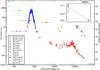 |
Fig. 1 Optical and X-ray (1 keV) light curves. Horizontal error bars represent the exposure times. Dashed lines represent the time power law fits to the 4 TNG I-band detections and to the last 7 X-ray data points. The inserted box zooms in on the TNG I-band detections. |
3. Results
3.1. Optical and X-ray light curves: the jet-break
To produce the X-ray light curve shown in Fig. 1, the unabsorbed flux integral was computed over the energy range 0.3–10 keV, from which the X-ray flux densities at 1 keV were derived. The required spectral indices β are fitted for the window timing (WT) and photon-counting (PC) XRT modes and taken from the Swift-XRT spectrum repository (Evans et al. 2007).
The main feature of the XRT light curve is a giant flare that occurs on top of an underlying decaying afterglow, which obeys a power law F(t) ∝ t−α of time index α = 0.8 ± 0.2. Though it is not shown anymore in the current light curve found in the XRT repository, Falcone et al. (2006) report for their binned data that the pre-flare decay rate is maintained in the post-flare, up until to ~104 s after the GRB start time. The light curve then exhibits a flattening combined with two over-imposed rebrightenings at ≈3 × 10⁴ and ≈8 × 10⁴ s, respectively. The latter marks the onset of a steep decline, which could be a jet-break. From the shallow decay phase the light curve evolves directly into post-jet-break, not showing the less steep pre-jet-break phase (Panaitescu 2006).
Considering the available I-band data at a time t > 1.28 × 10⁵ s, the time decay index is α = 2.1 ± 0.6, when fitted with a power law. This late time decay must be a post-break decay, since the ANU telescope detection appears to constrain the early time decay to a slope shallower than that of the TNG.
When fitting the last seven X-ray time bins with a power law, the result is α = 2.1 ± 0.3. The first of these seven bins matches the start of our optical observations at ~1.28 × 10⁵ s. If considering one extra earlier bin, i.e., for t > 1.1 × 10⁵ s (like in Falcone et al. 2006), the time index is then α = 2.3 ± 0.3, while Falcone et al. (2006) got a power law time index of α = 2.8 ± 0.8.
The results presented in this work are compatible with those from Falcone et al. (2006), despite using a slightly different X-ray data binning. From the currently available Swift-XRT data repository, it can be established that for the last seven bins, the count rate light curve has a minimum of 17 and a maximum of 99 counts per bin. Thus such binning is statistically meaningful.
The steep optical decay overlaps in time and has a time index consistent (within errors) with that in the X-rays, so the data suggest a jet-break.
The spectral index in any given band across a jet-break should remain unchanged. Therefore, in order to test the jet-break hypothesis, an averaged spectrum was created in the Swift-XRT repository for all points with t > 1.1 × 10⁵ s, resulting in a spectral index of  , with a best-fit value in excess of the Galactic hydrogen column density of
  cm-2. For the interval [~1000, 20 000] s, the spectral index is basically the same, with
  .
.
3.2. The spectral energy distribution
The broadband spectral energy distribution (SED) was computed at the epoch of our single R-band detection. Since the R-band point precedes the closest I-band point by ~1 h, the I-band post-jet-break slope was used to extrapolate the I-band value (0.04 mag brighter) at the R-band observation time. The effective wavelengths, λ0, corresponding to the R and I bands, were taken from Fukugita et al. (1995). The X-ray data point used in the SED has a flux density (at 1 keV) of 9 × 10⁻³ μJy, at the time of the penultimate bin point in the X-ray light curve. This X-ray bin point matches the extrapolated I-band and observed R-band observation time.
Fitting the broadband SED with a simple Fν(ν) ∝ ν−β power law yields a spectral index βOX = 0.9 ± 0.1. This value is consistent with the X-ray spectral index (Sect. 3.1). There is therefore no indication of a break between the optical and X-ray spectra and the SED between the I-band and ~5 keV is described well by a single power law with βOX = 0.9 ± 0.1.
Finally, although there is only one epoch at which the broadband SED could be computed, the temporal decay indices in the optical and X-rays are consistent as well, which is a necessary condition to keep having βX consistent with βOX in other epochs. In fact, if the optical and X-ray decay indices become different, it would necessarily imply a spectral break between optical and X-rays.
3.3. The closure relations
Considering the fireball synchrotron shock model as the major radiation mechanism responsible for the afterglows (e.g., Zhang & Mészáros 2004) and following, e.g., Sari et al. (1998), GRB 050502B roughly obeys the closure relations for a model of a uniform jet (valid for both ISM and wind cases) in a typical slow cooling regime, for ν > νc, where νc is the synchrotron cooling frequency. The electron power law index, p, is deduced from the temporal decay index at the post-jet-break phase, i.e., Fν ∝ t−p. Thus for p ~ 2.1 and βOX = 0.9 ± 0.1, within errors, α = 2β is observed.
3.4. Photometric redshift
The quasi-simultaneous R and I bands TNG observations at 215.6 and 219.2 ks, respectively, result in R − I = 1.12 ± 0.23 mag. The correction for simultaneity (using the time index computed for the I- band) is smaller than the error due to the uncertainty in the photometry, resulting in R − I = (1.16 ± 0.23) mag. This very red colour hints at either high redshift or high extinction in the host, or both. These possibilities were explored using the HyperZ photometric redshift code from Bolzonella et al. (2000). No reddening in the host and a fixed βOX = 0.9 ± 0.1 produce the best fitting result of z = 5.2 ± 0.3 (see Fig. 2). Since βOX and βX are consistent, this further favours the unextinguished model.
3.5. Burst energetics
According to Cummings et al. (2005), the fluence in the BAT range (15–350 keV) is Fγ = (8.0 ± 1.0) × 10-7 erg cm-2. To estimate the energy of the burst if occurring at z = 5.2, the corresponding luminosity distance is computed in a concordance cosmology model (Spergel et al. 2003). With H0 = 71 km s-1 Mpc-1, ΩM = 0.27 and ΩΛ = 0.73, then DL = 49.84 Gpc. For the BAT range of energies, considering the errors in the fluence and redshift, this results in an isotropic-equivalent energy of  erg, which is a typical value for long GRBs.
The jet opening angle θ, which is dependent on the redshift and jet-break time, can also be computed. To compare our results with θ ~ 8.1° from Falcone et al. (2006), the same formula is followed, other than a small correction, required for consistency of dimensionality, where n0 = nism/(1 cm-3). Thus where Falcone et al. (2006) assume z = 1 and E52 = 1, in ![Mathematical equation: \hbox{$\theta = 7.8\degr t_{5}^{3/8}\ E_{52}^{-1/8}\ n_{0}^{1/8}\ [(1+z)/2]^{-3/8}$}](/articles/aa/full_html/2011/02/aa13965-09/aa13965-09-eq126.png) , it is now t5 = 1.1, for a jet-break time of ~1.1 × 10⁵ s, E52 = 3.8ηγ, n0 ~ 1, for a uniform external interstellar medium density, and z = 5.2; this gives θ ~ 3.7°. As in other works (e.g., Ghirlanda et al. 2007; Frail et al. 2001), ηγ = 0.2 corresponds to an assumed radiative efficiency of 20%. Given that the bolometric Eγ,iso must be larger than the energy observed within the BAT range used here, θ ~ 3.7° is thus an upper limit, within the typically observed jet opening angles (Ghirlanda et al. 2007).
, it is now t5 = 1.1, for a jet-break time of ~1.1 × 10⁵ s, E52 = 3.8ηγ, n0 ~ 1, for a uniform external interstellar medium density, and z = 5.2; this gives θ ~ 3.7°. As in other works (e.g., Ghirlanda et al. 2007; Frail et al. 2001), ηγ = 0.2 corresponds to an assumed radiative efficiency of 20%. Given that the bolometric Eγ,iso must be larger than the energy observed within the BAT range used here, θ ~ 3.7° is thus an upper limit, within the typically observed jet opening angles (Ghirlanda et al. 2007).
4. Discussion
4.1. Optical and X-ray light curves: the jet-break
The second and last bump on the X-ray light curve masks the true start of the jet-break, while a possible bump or small flare can not be ruled out in the optical. There is a small increase in brightness in the first three I-band data points, but it is not significant given that the first point does not have the best S/N. Also the second and third I-band data points are consistent, within errors, with no flaring, as can be seen better in the zoomed inserted box in Fig. 1. Even if this was a flare, in order to explain the rapid decay from the first 3 detections in May 3 (starting at 128 796 s after the trigger) to the following detection in May 4 (at 219 235 s), occurring simultaneously in the X-rays, the jet-break still seems the best answer.
It is interesting to compare the last X-ray bump with the complex light curve of GRB 071010A (Covino et al. 2008), where after a rebrightening at 0.6 days after the trigger, a steeper decay began both in the X-ray and optical, as evidence of a jet-break. In this and other GRBs with similar light curves, there is no plateau phase prior to the bump though – and rebrightening explanations related to the density profile of the circumburst medium have been invoked (among others).
The optical post-jet-break slope could have been further constrained if earlier data had been taken, since the fitting of the X-ray jet-break data points starts some ~33 min (2000 s) earlier than our first optical data point. Also the TNG I-band non-detection at the significance of 2σ (i.e., the UL of May 5, 2005, at ~302 ks post-burst) favours an even steeper post-jet-break.
4.2. Photometric redshift
When considering extinction in the host with data from only two filters, it is impossible to strongly constrain both the redshift and AV, given that they are generically anticorrelated, as shown in Fig. 2. Several host extinction models were used with HyperZ and in Fig. 2 the Small Magellanic Cloud (SMC) model is shown as an example to illustrate the dependence with redshift. This suggests that a low redshift is allowed for high AV values.
As noted by Falcone et al. (2006), during the observations the total NH can be considered constant at approximately the Dickey & Lockman (1990) value for the Galactic hydrogen column density, NH = 3.6 × 1020 cm-2. Constructed with data from the XRT repository, a time-averaged spectrum between T0 + 68 and ~1.4 × 10⁵ s is best fitted (assuming z = 0) with an absorbed power law model where 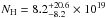 cm-2. This is a typical intrinsic excess value, similar to those observed in the high-redshift GRBs sample of Grupe et al. (2007). Within the XRT fit error, this result is consistent with zero, but taking the upper error value allows computing an upper limit on the possible excess extinction.
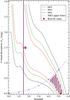 |
Fig. 2 Intrinsic reddening vs. redshift dependence, for an SMC extinction curve with SED slope fixed to β = 0.9. The 68%, 90% and 99% confidence contours are plotted. The XRT-fit line represents the AV upper limits, converted as described in the text. The maroon shaded area represents the 1σ region of the contour plot constrained by the XRT upper limits. The vertical line at z = 1.5 represents the VLT lower limit due to the lack of a host detection. |
There is no exactly known relation between AV and NH in GRB environments. To find the dependence of the AV ULs with z, the X-ray spectral fitting package Xspec (Arnaud 1996) was used, placing the excess NH column at redshifts of 0, 1, 2, 3, 4 and 5. The cubic polynomial that represents the XRT UL curve in Fig. 2 fits the data points obtained from the Milky-Way-based Predehl & Schmitt (1995) relation, where NH = 1.79 AV × 1021 cm-2. Although, in general, high NH corresponds to high AV, the dust-to-gas ratio in GRB hosts can be different and normally is lower than in the Milky Way. Galama & Wijers (2001) report some examples with high NH but with AV 10–100 times smaller than expected. Likewise the sample of Stratta et al. (2004) favours a dust-to-gas ratio of ~1/10 that of the Milky Way, as in an SMC environment. Therefore a more reasonable approach was to scale down by a factor of 10 the XRT UL data points presented in Fig. 2, after being computed from the Predehl & Schmitt (1995) relation.
Stressing that all the Xspec results are compatible with zero extinction, an inspection of Fig. 2, e.g., for z = 4 at the 1σ level, nevertheless shows an UL of AV ~ 0.5 mag. This is a relatively high extinction, which can not be probed directly at the rest frame by XRT, due to its spectral coverage. Therefore a combination of both high redshift and AV can also not be excluded and a more conservative result of z > 4 should be considered.
The GRB AV distribution is poorly constrained. While in the past samples were biased towards low extinction bursts, showing typical intrinsic reddening to be well below AV ~ 0.5 mag (Kann et al. 2006), recent observations provide evidence of highly reddened afterglows (Watson et al. 2006; Rol et al. 2007; Krühler et al. 2008; Elíasdóttir et al. 2009; Prochaska et al. 2009). The case of GRB 070306, detected initially in the K-band, is a remarkable example of a highly reddened burst with z = 1.496 and suggested AV = 5.6 mag (Jaunsen et al. 2008). Tanvir et al. (2008) report GRB 060923A as another similar extreme case.
As an additional note, since dust mostly affects the rest frame UV, normally a somewhat higher redshift (~2−3) is needed to get such R − I red colour. Furthermore, in the sample of Schady et al. (2007), all highly reddened bursts due to intrinsic extinction have large NH in the XRT data, which is the opposite of the present case.
For z > 4.5, UVOT can not detect the Lyman limit (Roming et al. 2005) and the UVOT data do not indicate any strong rebrightening in the optical simultaneous to the giant X-ray flare. Note however that, independent of its origin, the very red colour only strictly suggests very little flux in the blue and UV bands probed by UVOT, hence the occurrence of a dimmer optical flare can not be totally excluded.
If allowing for the possibility that there is no correlation between AV and NH (e.g., Jakobsson et al. 2006; Watson et al. 2007), the constraint from the X-ray spectrum could be circumvented. In this case, however, the extinction-corrected optical fluxes would be increasingly above the 0.9 power law extrapolation from the X-ray band, thus producing a convex SED. Such an SED shape has not been proposed within any afterglow model, has never been observed and seems therefore an extremely unlikely option.
Regarding the R-band VLT data, since GRB host galaxies can be very faint (e.g, Le Floc’h et al. 2003), the VLT non-detection of a host galaxy provides only a mild limit on the redshift. It is difficult to quantify a lower limit given the scarcity of data, but looking into samples of GRB host galaxies, such as in those of Wainwright et al. (2007) and Savaglio et al. (2009), hosts with magnitude R ≳ 26 typically have z ≳ 1.5. This can be taken as a rough lower limit to the redshift of GRB 050502B (Malesani et al. 2009).
4.3. Burst energetics
In Sect. 3.5, Eγ,iso was computed for z = 5.2. Just for reference, if taking z = 1, then Eγ,iso = 2.1 × 1051 erg, which compared to samples of other bursts with known redshift (e.g., Amati et al. 2008), would put GRB 050502B to the lower energy end of GRBs.
A hard question to answer is how to compute a bolometric rest frame isotropic-equivalent energy with a proper k-correction without knowing the value of the peak energy, Ep, exactly. Following Cummings et al. (2005) and Sakamoto et al. (2008), the BAT spectrum (range 15–350 keV) is well fitted by a single power law with a photon index Γ = 1.59 ± 0.14. From the BAT spectrum, ~90 keV is roughly the highest energy at which a reasonable detection still occurs and, given the value of Γ, this could be assumed as a lower limit for Ep. An empiric estimator could be considered instead, as in Sakamoto et al. (2009), where log (Ep/1 keV) = 3.258−0.829 Γ. Combining the estimator’s own 1σ uncertainties and those in Γ, then leads to  keV. Taking z = 5.2, 2.5 and Γ as the high and low-energy indices, respectively, of a Band function spectral shape (Band et al. 1993), already results in a large ~200 keV uncertainty range for the rest frame peak energy,
  keV, if considering only the uncertainties in Γ. These estimators are only valid for BAT spectra that can be fitted by a single power law, but older empiric estimators produce significantly different results (e.g. Liang et al. 2007).
To check that GRB 050502B obeys the Amati and Ghirlanda relations, the “standard” isotropic-equivalent bolometric energy release in the rest frame range of 1 keV to 10 MeV needs to be computed. It is difficult to reach firm conclusions given the errors in Fγ, Γ, z and the uncertainties in both Ep and the Band function indices. In a time dilation and k-correction computation (Amati et al. 2002), different combinations of parameters produce significantly different results. For reference, an exercise within the parameters errors, say with Fγ = 9 × 10⁻⁷ erg cm-2, z = 5.5, Band energy indices β = 2.5, α = 1.7 and Ep = 70 keV, produces a very reasonable Ep,i = 455 keV and Eγ,iso = 9.3 × 1052 erg. Following one of the latest GRB samples to test the Amati relation (Amati et al. 2008), this result places GRB 050502B right in the middle zone of the Ep,i vs. Eγ,iso plot-validating sample. This energy corresponds to a typical GRB, which is ~40 times smaller than the corresponding Eγ,iso inferred for the extreme case of GRB 080916C (Abdo et al. 2009; Greiner et al. 2009), the most energetic GRB known to date.
Since the presence of a jet-break suggests a conical GRB geometry, the true gamma-ray energy release, Eγ, is less than Eγ,iso , with Eγ = fb Eγ,iso (Frail et al. 2001; Sari et al. 1999). For the above choice of parameters, computing the beaming fraction, fb = 1 − cosθ, with the Eγ,iso corresponding newly calculated angle (θ ~ 3.2°), results in Eγ = 1.45 × 1050 erg. Two comments can be made at this point:
-
1)
This rather low total energy sug-gests that the relatively high redshift ofz = 5.2 can not be overly high;
-
2)
This value is lower than the average of those reported in earlier surveys, clustering around the GRBs “standard” energy reservoir (e.g. Frail et al. 2001). As observed later by Ghirlanda et al. (2004) in more recent and larger GRB samples, this clustering is in fact not so narrow, covering about 2 orders of magnitude.
5. Conclusions
As a main conclusion the data favour the high redshift nature of GRB 050502B. While even a very red colour is not sufficient to claim a high redshift (see, e.g., GRB 060923A, GRB 070306), in this case an extra constraint is provided by βOX being consistent with βX. Also there is no significant excess NH and the post-jet-break slope αX is consistent with αopt, again favouring a single component origin for the two bands. The consistency of the time indices favours the other main conclusion: the existence of an achromatic jet-break.
The scarcity of optical data limits a deeper discussion regarding the late engine model as an explanation for the X-ray giant flare and later activity (Falcone et al. 2006) and likewise in considering alternative models. It is interesting to note however, that the jet-break appears after the end of the last bump, which could also be caused by later engine activity. No transition is observed from the shallow phase to a pre-jet-break phase, likely because the extra “late prompt” component is added to the fireball model component. As the effects of the late engine activity cease, the afterglow then shows a standard jet-break.
Given the high-redshift nature of GRB 050502B, its consequent afterglow red R − I colour and the fact that typical X-ray flares emit most of their flux in the γ-ray and X-ray bands (e.g. Page et al. 2007; Krühler et al. 2009), it is not very surprising that the simultaneous UVOT observation do not show evidence of strong rebrightening in the optical wavelength regime contemporaneous with the prominent X-ray flare.
Finally it is interesting to consider that for z = 5.2 ± 0.3, this would be one of the highest redshift observed achromatic breaks, when compared to the samples of Liang et al. (2008) and Ghirlanda et al. (2007).
Acknowledgments
E.P. acknowledges financial support from contracts PRIN INAF 2006 and ASI I/088/06/0. The Dark Cosmology Centre is funded by the Danish National Research Foundation. T.K. acknowledges support by the DFG cluster of excellence “Origin and Structure of the Universe”. This work made use of data supplied by the UK Swift Science Data Centre at the University of Leicester. We thank G. Szokoly, D. Burlon and G. Ghirlanda for useful discussions and V. Sudilovski and K. Dzurella for improvements in the draft.
References
- Abdo, A. A., Ackermann, M., Arimoto, M., et al. 2009, Science, 323, 1688 [Google Scholar]
- Amati, L., Frontera, F., Tavani, M., et al. 2002, A&A, 390, 81 [NASA ADS] [CrossRef] [EDP Sciences] [Google Scholar]
- Amati, L., Guidorzi, C., Frontera, F., et al. 2008, MNRAS, 391, 577 [NASA ADS] [CrossRef] [MathSciNet] [Google Scholar]
- Arnaud, K. A. 1996, in Astronomical Data Analysis Software and Systems V, ed. G. H. Jacoby, & J. Barnes, ASP Conf. Ser., 101, 17 [Google Scholar]
- Band, D., Matteson, J., Ford, L., et al. 1993, ApJ, 413, 281 [NASA ADS] [CrossRef] [Google Scholar]
- Barthelmy, S. D., Barbier, L. M., Cummings, J. R., et al. 2005, Space Sci. Rev., 120, 143 [NASA ADS] [CrossRef] [Google Scholar]
- Bhatt, B. C., Ramya, S., & Anupama, G. C. 2005, GCN, 3346 [Google Scholar]
- Bolzonella, M., Miralles, J.-M., & Pelló, R. 2000, A&A, 363, 476 [NASA ADS] [Google Scholar]
- Burrows, D. N., Hill, J. E., Nousek, J. A., et al. 2005a, Space Sci. Rev., 120, 165 [NASA ADS] [CrossRef] [Google Scholar]
- Burrows, D. N., Romano, P., Falcone, A., et al. 2005b, Science, 309, 1833 [NASA ADS] [CrossRef] [PubMed] [Google Scholar]
- Cardelli, J. A., Clayton, G. C., & Mathis, J. S. 1989, ApJ, 345, 245 [NASA ADS] [CrossRef] [Google Scholar]
- Cenko, S. B., Fox, D. B., Rich, J., et al. 2005, GCN, 3358 [Google Scholar]
- Chonis, T. S., & Gaskell, C. M. 2008, AJ, 135, 264 [NASA ADS] [CrossRef] [Google Scholar]
- Covino, S., D’Avanzo, P., Klotz, A., et al. 2008, MNRAS, 388, 347 [NASA ADS] [CrossRef] [Google Scholar]
- Cummings, J., Barbier, L., Barthelmy, S., et al. 2005, GCN, 3339 [Google Scholar]
- Dickey, J. M., & Lockman, F. J. 1990, ARA&A, 28, 215 [NASA ADS] [CrossRef] [MathSciNet] [Google Scholar]
- Elíasdóttir, Á., Fynbo, J. P. U., Hjorth, J., et al. 2009, ApJ, 697, 1725 [NASA ADS] [CrossRef] [Google Scholar]
- Evans, P. A., Beardmore, A. P., Page, K. L., et al. 2007, A&A, 469, 379 [NASA ADS] [CrossRef] [EDP Sciences] [Google Scholar]
- Falcone, A. D., Burrows, D. N., Lazzati, D., et al. 2006, ApJ, 641, 1010 [NASA ADS] [CrossRef] [Google Scholar]
- Frail, D. A., Kulkarni, S. R., Sari, R., et al. 2001, ApJ, 562, L55 [NASA ADS] [CrossRef] [Google Scholar]
- Fukugita, M., Shimasaku, K., & Ichikawa, T. 1995, PASP, 107, 945 [NASA ADS] [CrossRef] [Google Scholar]
- Galama, T. J., & Wijers, R. A. M. J. 2001, ApJ, 549, L209 [NASA ADS] [CrossRef] [Google Scholar]
- Gehrels, N., Chincarini, G., Giommi, P., et al. 2004, ApJ, 611, 1005 [NASA ADS] [CrossRef] [Google Scholar]
- Ghirlanda, G., Ghisellini, G., & Lazzati, D. 2004, ApJ, 616, 331 [NASA ADS] [CrossRef] [Google Scholar]
- Ghirlanda, G., Nava, L., Ghisellini, G., & Firmani, C. 2007, A&A, 466, 127 [NASA ADS] [CrossRef] [EDP Sciences] [Google Scholar]
- Ghisellini, G., Nardini, M., Ghirlanda, G., & Celotti, A. 2009, MNRAS, 393, 253 [NASA ADS] [CrossRef] [Google Scholar]
- Greiner, J., Clemens, C., Krühler, T., et al. 2009, A&A, 498, 89 [NASA ADS] [CrossRef] [EDP Sciences] [Google Scholar]
- Grupe, D., Nousek, J. A., van den Berk, D. E., et al. 2007, AJ, 133, 2216 [NASA ADS] [CrossRef] [Google Scholar]
- Jakobsson, P., Fynbo, J. P. U., Ledoux, C., et al. 2006, A&A, 460, L13 [NASA ADS] [CrossRef] [EDP Sciences] [Google Scholar]
- Jaunsen, A. O., Rol, E., Watson, D. J., et al. 2008, ApJ, 681, 453 [NASA ADS] [CrossRef] [Google Scholar]
- Kann, D. A., Klose, S., & Zeh, A. 2006, ApJ, 641, 993 [NASA ADS] [CrossRef] [Google Scholar]
- Krühler, T., Küpcü Yoldaş, A., Greiner, J., et al. 2008, ApJ, 685, 376 [NASA ADS] [CrossRef] [Google Scholar]
- Krühler, T., Greiner, J., McBreen, S., et al. 2009, ApJ, 697, 758 [NASA ADS] [CrossRef] [Google Scholar]
- Landolt, A. U. 1992, AJ, 104, 340 [NASA ADS] [CrossRef] [Google Scholar]
- Le Floc’h, E.,Duc, P.-A., Mirabel, I. F., et al. 2003, A&A, 400, 499 [NASA ADS] [CrossRef] [EDP Sciences] [Google Scholar]
- Liang, E.-W., Zhang, B.-B., & Zhang, B. 2007, ApJ, 670, 565 [NASA ADS] [CrossRef] [Google Scholar]
- Liang, E.-W., Racusin, J. L., Zhang, B., Zhang, B.-B., & Burrows, D. N. 2008, ApJ, 675, 528 [NASA ADS] [CrossRef] [Google Scholar]
- Malesani, D., Hjorth, J., Fynbo, J. P. U., et al. 2009, AIP Conf. Ser. 1111, ed. G. Giobbi, A. Tornambe, G. Raimondo, M. Limongi, L. A. Antonelli, N. Menci, & E. Brocato, 513 [Google Scholar]
- Misra, K., & Pandey, S. B. 2005, GCN, 3350 [Google Scholar]
- Nardini, M., Ghisellini, G., Ghirlanda, G., & Celotti, A. 2010, MNRAS, 403, 1131 [NASA ADS] [CrossRef] [Google Scholar]
- O’Donnell, J. E. 1994, ApJ, 422, 158 [NASA ADS] [CrossRef] [Google Scholar]
- Pagani, C., Falcone, A., Burrows, D. N., et al. 2005, GCN, 3333 [Google Scholar]
- Page, K. L., Willingale, R., Osborne, J. P., et al. 2007, ApJ, 663, 1125 [NASA ADS] [CrossRef] [Google Scholar]
- Panaitescu, A. 2006, Nuovo Cimento B Serie, 121, 1099 [NASA ADS] [Google Scholar]
- Predehl, P., & Schmitt, J. H. M. M. 1995, A&A, 293, 889 [NASA ADS] [Google Scholar]
- Prochaska, J. X., Sheffer, Y., Perley, D. A., et al. 2009, ApJ, 691, L27 [NASA ADS] [CrossRef] [Google Scholar]
- Rhoads, J. E. 1997, ApJ, 487, L1 [NASA ADS] [CrossRef] [Google Scholar]
- Rich, J., Schmidt, B., & Christiansen, J. 2005a, GCN, 3338 [Google Scholar]
- Rich, J., Schmidt, B., & Christiansen, J. 2005b, GCN, 3331 [Google Scholar]
- Rol, E., van der Horst, A., Wiersema, K., et al. 2007, ApJ, 669, 1098 [NASA ADS] [CrossRef] [Google Scholar]
- Roming, P. W. A., Kennedy, T. E., Mason, K. O., et al. 2005, Space Sci. Rev., 120, 95 [NASA ADS] [CrossRef] [Google Scholar]
- Roming, P. W. A., Koch, T. S., Oates, S. R., et al. 2009, ApJ, 690, 163 [NASA ADS] [CrossRef] [Google Scholar]
- Sakamoto, T., Barthelmy, S. D., Barbier, L., et al. 2008, ApJS, 175, 179 [NASA ADS] [CrossRef] [Google Scholar]
- Sakamoto, T., Sato, G., Barbier, L., et al. 2009, ApJ, 693, 922 [NASA ADS] [CrossRef] [Google Scholar]
- Sanchawala, K., Wu, W. L., Huang, K. Y., et al. 2005, GCN, 3334 [Google Scholar]
- Sari, R., Piran, T., & Narayan, R. 1998, ApJ, 497, L17 [NASA ADS] [CrossRef] [Google Scholar]
- Sari, R., Piran, T., & Halpern, J. P. 1999, ApJ, 519, L17 [NASA ADS] [CrossRef] [Google Scholar]
- Sasaki, M., Manago, N., Noda, K., & Asaoka, Y. 2005, GCN, 3421 [Google Scholar]
- Savaglio, S., Glazebrook, K., & LeBorgne, D. 2009, ApJ, 691, 182 [NASA ADS] [CrossRef] [MathSciNet] [Google Scholar]
- Schady, P., Falcone, A., Holland, S., et al. 2005, GCN, 3337 [Google Scholar]
- Schady, P., Mason, K. O., Page, M. J., et al. 2007, MNRAS, 377, 273 [NASA ADS] [CrossRef] [Google Scholar]
- Schlegel, D. J., Finkbeiner, D. P., & Davis, M. 1998, ApJ, 500, 525 [NASA ADS] [CrossRef] [Google Scholar]
- Spergel, D. N., Verde, L., Peiris, H. V., et al. 2003, ApJS, 148, 175 [NASA ADS] [CrossRef] [Google Scholar]
- Stratta, G., Fiore, F., Antonelli, L. A., Piro, L., & De Pasquale, M. 2004, ApJ, 608, 846 [NASA ADS] [CrossRef] [Google Scholar]
- Tanvir, N. R., Levan, A. J., Rol, E., et al. 2008, MNRAS, 388, 1743 [NASA ADS] [CrossRef] [Google Scholar]
- Tody, D. 1993, in Astronomical Data Analysis Software and Systems II, ed. R. J. Hanisch, R. J. V. Brissenden, & J. Barnes, ASP Conf. Ser., 52, 173 [Google Scholar]
- Torii, K. 2005, GCN, 4113 [Google Scholar]
- Wainwright, C., Berger, E., & Penprase, B. E. 2007, ApJ, 657, 367 [NASA ADS] [CrossRef] [Google Scholar]
- Watson, D., Fynbo, J. P. U., Ledoux, C., et al. 2006, ApJ, 652, 1011 [NASA ADS] [CrossRef] [Google Scholar]
- Watson, D., Hjorth, J., Fynbo, J. P. U., et al. 2007, ApJ, 660, L101 [NASA ADS] [CrossRef] [Google Scholar]
- Zhang, B., & Mészáros, P. 2004, Int. J. Mod. Phys. A, 19, 2385 [NASA ADS] [CrossRef] [Google Scholar]
All Tables
All Figures
|
Fig. 1 Optical and X-ray (1 keV) light curves. Horizontal error bars represent the exposure times. Dashed lines represent the time power law fits to the 4 TNG I-band detections and to the last 7 X-ray data points. The inserted box zooms in on the TNG I-band detections. |
| In the text | |
|
Fig. 2 Intrinsic reddening vs. redshift dependence, for an SMC extinction curve with SED slope fixed to β = 0.9. The 68%, 90% and 99% confidence contours are plotted. The XRT-fit line represents the AV upper limits, converted as described in the text. The maroon shaded area represents the 1σ region of the contour plot constrained by the XRT upper limits. The vertical line at z = 1.5 represents the VLT lower limit due to the lack of a host detection. |
| In the text | |
Current usage metrics show cumulative count of Article Views (full-text article views including HTML views, PDF and ePub downloads, according to the available data) and Abstracts Views on Vision4Press platform.
Data correspond to usage on the plateform after 2015. The current usage metrics is available 48-96 hours after online publication and is updated daily on week days.
Initial download of the metrics may take a while.