| Issue |
A&A
Volume 525, January 2011
|
|
|---|---|---|
| Article Number | A88 | |
| Number of page(s) | 5 | |
| Section | The Sun | |
| DOI | https://doi.org/10.1051/0004-6361/201015476 | |
| Published online | 02 December 2010 | |
Separation of drifting pulsating structures in a complex radio spectrum of the 2001 April 11 event
1
Astronomical Institute of the Academy of Sciences of the Czech
Republic,
25165
Ondřejov,
Czech Republic
e-mail: This email address is being protected from spambots. You need JavaScript enabled to view it.
2
Astronomical Institute, Slovak Academy of Sciences,
05960
Tatranská Lomnica, Slovak
Republic
Received: 27 July 2010
Accepted: 12 October 2010
Abstract
Aims. We present new method of separating a complex radio spectrum into single radio bursts. The method is used in the analysis of the 0.8–2.0 GHz radio spectrum of the 2001 April 11 event, which was rich in drifting pulsating structures.
Methods. The method is based on the wavelet analysis technique, which separates different spatial-temporal components (radio bursts) that are difficult to recognize in the original radio spectrum.
Results. We show with this method that the complex radio spectrum observed during the 2001 April 11 event consists of at least four drifting pulsating structures (DPSs). These structures were separated with respect to their different frequency drifts. The DPSs indicate at least four plasmoids that are supposed to be formed in a flaring current sheet.
Key words: Sun: corona / Sun: flares / Sun: radio radiation / Sun: oscillations
© ESO, 2010
1. Introduction
The drifting pulsating structures (DPSs, Karlický 2004; Reiner et al. 2008; Karlický et al. 2010a), which were observed at the beginning of the eruptive solar flares in the 0.8−2.0 GHz frequency range, have been found to be radio signatures of plasmoid ejections (Karlický & Odstrčil 1994; Ohyama & Shibata 1998; Kliem et al. 2000; Khan et al. 2002; Karlický et al. 2002). Similarly, Hudson et al. (2001) identified a rapidly moving hard X-ray source, observed by the Yohkoh/HXT, together with the moving microwave source and plasmoid ejection seen in the Yohkoh/SXT images. An association with the high-frequency slowly drifting burst was reported. Furthermore, Kundu et al. (2001) observed two moving Yohkoh soft X-ray ejections accompanied by moving decimetric/metric radio sources observed by Nancay radioheliograph.
Based on the MHD numerical simulations, Kliem et al. (2000) suggested that the drifting pulsation structure is generated by superthermal electrons, trapped in the magnetic island (plasmoid) in the bursty regime of the magnetic field reconnection. The global slow negative frequency drift of the structure was explained by a plasmoid propagation upward in the solar corona toward lower plasma densities. This MHD model of DPSs was further developed and verified by Bárta et al. (2008a,b, 2010). On the other hand, details of the emission processes in DPSs were studied by the particle-in-cell models (Karlický & Bárta 2007; Karlický et al. 2010b).
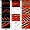 |
Fig. 1 Test of separation of bursts (artificial dynamic spectrum, duration = 80 s, frequency range = 0.8−2.0 GHz). Four different artificial DPSs are shown in the panels a − d), for their parameters see Table 1. The sum of these DPSs plus four other pulsations (Table 1) is shown in panel e). Panel f) shows the averaged global wavelet spectrum (ASf) with a peak for the frequency width = 400 MHz, panel g) the filtered spectrum ASf in the frequency width range 220−500 MHz, and panel h) the averaged global wavelet spectrum (ASt) made from the spectrum in panel g) with peaks for the temporal periods P = 2, 4, 8, 15 and 42 s. The panels i − l) show the final separated spectra: i) separated pulsations in the P-range 2.9−5.7 s, j) separated pulsations in the P-range 5.7−10.0 s, k) separated pulsations in the P-range 10−24 s, and l) separated pulsations in the P-range 24−90 s. The positive and negative parts of amplitudes (in relation to their mean values) are in white and black, respectively (panels g) and i − l)). The arrows show the frequency drifts D (Table 1). |
When the DPSs, corresponding to different plasmoids, are produced at close frequencies in similar time intervals, then the observed radio spectrum is very complex; sometimes DPSs are even superimposed on other types of bursts and fine structures. Therefore, it is highly desirable to separate these bursts and analyze them separately. A first attempt in this field was made by Sych et al. (2006), where they used the wavelet filtration method for the narrowband spikes and pulsations. Here we developed a new and more extended method for the same purpose that is able to separate the bursts and fine structures not only according to frequency widths, but also according to their temporal scales and even according to their frequency drifts.
We describe here how first the method was tested using artificial radio spectra. Then we applied this method to the real radio spectrum (observed during the 2001 April 11 event by the Ondřejov radiospectrograph), which was very rich in drifting pulsating structures.
2. Separation method
Our new method is based on the wavelet analysis technique (Torrence & Compo 1998; Morlet mother function, parameter ω = 6, significance level = 99%). It consists of two independent parts that separate different components of the radio spectrum (bursts and their fine structures): (i) according to their frequency bandwidth; and (ii) according to their temporal scales.
In the first part, a series of wavelet power spectra (WPS) of radio fluxes are computed along all cuts of the radio spectrum at specific time moments. From this series we determined series of 1-D global wavelet spectra (GWS). Then we computed a 1-D averaged global wavelet spectrum (ASf) by averaging the GWS. It gives us information about the characteristic frequency widths (bandwidths) that are present in the spectrum under study. Then the original radio spectrum is filtered with respect to these characteristic frequency width(s) (inverse wavelet analysis, Torrence & Compo 1998), and one or more new separated radio spectra are calculated. These spectra consist of only those components (bursts) with the required frequency width.
Similarly, in the second part, a series of wavelet power spectra (WPS) of radio fluxes are computed along all cuts of the radio spectrum at specific frequencies. From this series we determined series of 1-D global wavelet spectra (GWS) and by their averaging computed the 1-D averaged global wavelet spectrum (ASt). It gives us information about the characteristic temporal periods that are present in the spectrum. Then the original radio spectrum is filtered with respect to these characteristic temporal period(s). Thus one or more new separated radio spectra that consist of only components (bursts) with the demanded characteristic period are calculated.
Parameters of the bursts used in a construction of the artificial radio spectrum.
We used two types of presentation of the dynamic radio spectra (2-D plot frequency vs. time): (i) the original radio dynamic spectrum where the level of the quiet sun (background, about 50−100 SFU) represents the lowest values of the spectrum, which are shown in black (see Fig. 1, panel e). All values of bursts (radio emissions) have higher values than the background, and they are shown in red (minimal values of the burst, for example 120 SFU) and in white (maximal values of the burst, for example 600 SFU); (ii) filtered spectra. In the artificial (panels a − e in Fig. 1) or separated spectra (panels g, i − l in Fig. 1 and panels c, e − h in Fig. 2) only the bursts (without background) are presented. Then the maximum positive and negative parts of the flux amplitude (in relation to the mean flux value) are shown in white and black, respectively. The values more or less about zero are presented in red. This type of displaying enables us to see better the structure and frequency drifts of the separated bursts in the filtered spectra.
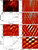 |
Fig. 2 Separation of real DPSs (2001 April 11 radio dynamic spectrum): a) original radio spectrum with DPSs; b) averaged global spectrum (ASf) with a peak for the frequency width = 450 MHz; c) radio spectrum filtered from ASf in the frequency width range = 290−540 MHz; d) averaged global spectrum (ASt) made from the spectrum in the panel c) with peaks for the periods P = 4.7, 8.5, 16.0, and 29.0 s; e) separated DPSs in the period range 2.2−5.5 s; f) separated DPSs in the period range 5.5−10.0 s; g) separated DPSs in the period range 10−20 s; and h) separated DPSs in the period range 20−44 s. Arrows in panels show frequency drifts of DPSs (see Sect. 3.2). The positive and negative parts of amplitudes (in relation to their mean values) are given in white and black, respectively (panels c) and e − h)). |
2.1. Separation of bursts in the artificial dynamic spectrum
To show the possibilities of our method we tested it on the artificial dynamic spectrum (Fig. 1, panel e), which was built to be similar to the observed radio spectra. The artificial radio spectrum includes a mixture of eight individual spectra (see Table 1 and the four examples in panels a − d of Fig. 1), where each spectrum has duration = 80 s, frequency range = 0.8−2.0 GHz, time and frequency resolutions = 0.1 s and 5 MHz, respectively. As is typical for observations, the spectra consist of DPSs with negative frequency drifts. As a background (quiet-sun level) we used a spectrum (No. 5 in Table 1) with the following parameters: frequency width (bandwidth) W = 20 MHz, period of individual pulsations P = 0.5 s and flux amplitude A = 50 arbitrary units. These pulsations uniformly overlay the whole dynamic spectrum (i.e. at all frequencies and in the whole time interval). Another three dynamic spectra (not shown here) contain various types of individual non-drifting pulsations with different frequency widths (Nos. 6−8 in Table 1).
Because we focused here on a detection of different global frequency drifts of DPSs, we used four artificial spectra (Nos. 1−4 in Table 1) with the drifts D = −120, −80, −30, and −10 MHz s-1 and the repetition period of these DPSs Pr = 4, 8, 15, and 42 s (panels a, b, c, and d in Fig. 1), respectively. The arrows in panels a − d mark the frequency drifts of DPSs D (see Table 1). The frequency width and period of all individual pulsations were chosen to be W = 400 MHz and P = 2 s (see the panels a − d in Fig. 1 and spectra Nos. 1−4 in Table 1).
The mixture of all these artificial spectra (Table 1) is shown in the panel e of Fig. 1. Here we can see mainly the DPSs with the highest flux amplitude A. This is similar to real radio spectra (Fig. 2, panel a). This artificial dynamic spectrum (Fig. 1, panel e) is an input data set for the separation procedure according to the frequency widths of individual bursts. The averaged wavelet spectrum (ASf) computed from all individual GWS of all individual time moments in the artificial dynamic spectrum shows a peak for the frequency width = 400 MHz (panel f, Fig. 1). It agrees with values in Table 1, where most of DPSs and pulsations have the frequency width W ≈ 400 MHz. Then we computed a new filtered spectrum in the frequency width range 220−500 MHz, where the values 220 and 500 MHz correspond to local minima around the peak at 400 MHz (Fig. 1, panel f). The new filtered spectrum is presented in panel g and consists of only the spectra Nos. 1−4 and 6 of Table 1.
Then this filtered spectrum became the input data set for the separation according to periods of the individual bursts. The averaged spectrum (ASt) computed from all individual GWS of all individual frequencies in the dynamic spectrum shows five peaks (panel h) for the period of individual pulsations P = 2 s as well as for the repetition period Pr = 4, 8, 15, and 42 s of DPSs. This result very well reflects the parameters of the input data set (spectra Nos. 1−4 and 6, Table 1). Then we computed the final filtered spectra for separated DPSs in the time period ranges 2.9−5.7 s (Fig. 1, panel i), 5.7−10.0 s (panel j), 10−24 s (panel k) and 24−90 s (panel l), where these values correspond to local minima around the peaks at 4, 8, 15, and 42 s (Fig. 1, panel h), respectively. The positive and negative parts of amplitudes (in the relation to their mean value) are expressed in white and black, respectively (Fig. 1, panels g and i − l).
These final filtered spectra (Fig. 1, panels i − l) are similar to the original ones in the panels a − d. We can see just the same number of DPSs and the same frequency drift. On the other hand, some deviations between the original spectra (Fig. 1, panels a − d) and final spectra (Fig. 1, panels i − l) can be seen. These deviations are generated because of the limitations of the wavelet method caused by a finite length of the time and frequency data cuts. In case of the separation according to the frequency widths the wavelet method extends the individual components (bursts) to the whole spectral range. For example, the original DPSs in panel c of Fig. 1 have the 1.2−1.9 GHz spectral range, but the final DPSs in the corresponding panel k have 0.8−2.0 GHz range. In the separation according to the temporal periods the wavelet method extends the individual components to the whole time interval. For example, the upper DPS in panel d of Fig. 1 lasts from 1 to 39 s, but in the corresponding panel l from 0 to 65 s. The bursts corresponding to the real DPSs in the initial spectra (Fig. 1, panels a − d) are shown as the brightest parts of the final spectra (Fig. 1, panels i − l). It is because of the highest wavelet power in the place of the real signal. Thus, we cannot establish the frequency range and time interval of the separated components exactly with this method, but only approximately. On the other hand, this test shows that the presented method can be used for the separation of DPSs superimposed in real radio spectra, especially on the base of their different frequency drifts.
3. Separation of bursts in the observed radio dynamic spectrum
3.1. Observational data
The 2001 April 11 flare (GOES X-ray class M2.3, maximum 13:26 UT, Hα importance 1F) was observed in the active region NOAA AR9415, in the position S22W27. The corresponding radio spectrum was recorded by the Ondřejov radiospectrograph (Jiřička et al. 1993). For our analysis we chose a part from the whole radio spectrum that lasted 80 s (13:07:50−13:09:10 UT) and had the time resolution 0.1 s in the frequency range 0.8−2.0 GHz (Fig. 2, panel a). This radio spectrum consists of several superimposed DPSs, which we try to separate as follows.
3.2. Separation of drifting pulsating structures (DPSs)
The procedure of separation of DPSs in the real radio spectrum was exactly the same as for the artificial spectrum. We took the radio dynamic spectrum with DPSs (Fig. 2, panel a) as an input data set for the separation according to their frequency widths. Then we computed the averaged wavelet spectrum (ASf) calculated from all GWS. It shows a peak for the frequency width 450 MHz (Fig. 2, panel b). This means that the most of the DPSs in the radio spectrum (panel a) have a frequency width of about 450 MHz. Therefore, we computed a new filtered radio spectrum in the frequency width range 290−540 MHz, where the values 290 and 540 MHz correspond to local minima around the peak at 450 MHz. This filtered spectrum is presented in panel c of Fig. 2.
Then the data set presented in panel c is taken as the input data set for the separation according to temporal periods of DPSs. The averaged global spectrum (ASt) computed from all GWS shows four peaks (panel d) for the periods P = 4.7, 8.5, 16.0, and 29.0 s. This means that most of the bursts with a frequency width about 450 MHz have a characteristic period of either 4.5, 8.7, 15, or 29 s. Then, using our method with the inverse wavelet transform we computed final spectra filtered in the period ranges 2.2−5.5 s (panel e), 5.5−10.0 s (panel f), 10−20 s (panel g), and 20−44 s (panel h), where these range values correspond to local minima around the period peaks (see panel d). The positive and negative parts of amplitudes are in white and black, respectively (panels c and e − h). This type of displaying makes it possible to see individual DPSs in very good contrast. The shortest period recognized here, the period P = 1.9 s, is the period of individual pulses in DPSs and thus is beyond the scope of this study.
At least four different frequency drifts can be recognized (−98, −52, −27, and −15 MHz s-1 – see the arrows 1, 2, 3, and 4 in the panels e, f, g, and h, respectively). This means that at least four DPSs are present in the complex radio spectrum observed in the 2001 April 11 event. Similar to the case of the artificial spectrum, the limited temporal and frequency ranges of DPSs and the spectrum itself cause false features. Also interferences among DPSs could play a role. Nevertheless, as shown by the previous test, the frequency drifts can be considered as real.
4. Conclusions
We present a new method for the separation of bursts in a complex radio dynamic spectrum. The method was successfully tested on the artificial radio spectrum with several superimposed bursts.
Then, using this method, the complex spectrum observed during the 2001 April 11 flare with many drifting pulsating structures (DPSs) was analyzed. We found that the characteristic bandwidth of these DPSs is about 450 MHz. On the other hand, these superimposed DPSs revealed the temporal periods 4.7, 8.5, 16.0, and 29.0 s, and frequency drifts −98, −52, −27, and −15 MHz s-1 (Fig. 2, panels e, f, g, and h, respectively).
This analysis shows that a mixture of DPSs (shown in Fig. 2, panel a) consists of at least of four different drifting pulsating structures. In accordance with the papers presented in the introduction, this means that at least four plasmoids (magnetic islands, magnetic ropes in 3D) are present in the flare current sheet, where the flare magnetic reconnection takes place. Because these plasmoids radiate on the plasma or double plasma frequencies, the plasma densities in these four plasmoids are similar (about 1.8 × 10¹⁰ or 4.4 × 109 cm-3 assuming the fundamental or harmonic emission frequency, respectively). But the velocities of these plasmoids, which are oriented in the upward direction in the solar atmosphere, differ. It resembles the observation of several interacting plasmoids in the 2001 April 18 flare (Karlický & Kliem 2010). In future this type of studies should be made in comparison with the spatially resolved plasmoids, e.g. by the new Brazilian dm-Radio Array (BDA, Sawant et al. 2002).
Acknowledgments
We thank the referee for very useful comments that improved the paper. H.M., M.K. acknowledge support from the Grant IAA300030701 of the Academy of Sciences of the Czech Republic and the research project AVOZ10030501 of the Astronomical Institute AS CR. The work of J.R. was partly supported by the Slovak Grant Agency VEGA (project 2/0064/09). The program of mobility between the academies of the Czech Republic and Slovakia is also acknowledged. The wavelet analysis was performed using the software based on tools provided by C. Torrence and G. P. Compo at http://paos.colorado.edu/research/wavelets.
References
- Bárta, M., Karlický, M., & Žemlička, R. 2008a, Sol. Phys., 253, 173 [NASA ADS] [CrossRef] [Google Scholar]
- Bárta, M., Vršnak, B., & Karlický, M. 2008b, A&A, 477, 649 [NASA ADS] [CrossRef] [EDP Sciences] [Google Scholar]
- Bárta, M., Büchner, J., & Karlický, M. 2010, Adv. Space Res., 45, 10 [NASA ADS] [CrossRef] [Google Scholar]
- Hudson, H. S., Kosugi, T., Nitta, N. V., & Shimojo, M. 2001, ApJ, 561, L211 [NASA ADS] [CrossRef] [Google Scholar]
- Jiřička, K., Karlický, M., Kepka, O., & Tlamicha, A. 1993, Sol. Phys., 147, 203 [NASA ADS] [CrossRef] [Google Scholar]
- Karlický, M. 2004, A&A, 417, 325 [NASA ADS] [CrossRef] [EDP Sciences] [Google Scholar]
- Karlický, M., & Bárta, M. 2007, A&A, 464, 735 [NASA ADS] [CrossRef] [EDP Sciences] [Google Scholar]
- Karlický, M., & Kliem, B. 2010, Sol. Phys., 266, 71 [NASA ADS] [CrossRef] [Google Scholar]
- Karlický, M., & Odstrčil, D. 1994, Sol. Phys., 155, 171 [NASA ADS] [CrossRef] [Google Scholar]
- Karlický, M., Fárník, F., & Mészárosová, H. 2002, A&A, 395, 677 [NASA ADS] [CrossRef] [EDP Sciences] [Google Scholar]
- Karlický, M., Zlobec, P., & Mészárosová, H. 2010a, Sol. Phys., 261, 281 [NASA ADS] [CrossRef] [Google Scholar]
- Karlický, M., Bárta, M., & Rybák, J. 2010b, A&A, 514, A28 [NASA ADS] [CrossRef] [EDP Sciences] [Google Scholar]
- Khan, J. I., Vilmer, N., Saint-Hilaire, P., & Benz, A. O. 2002, A&A, 388, 363 [NASA ADS] [CrossRef] [EDP Sciences] [Google Scholar]
- Kliem, B., Karlický, M., & Benz, A. O. 2000, A&A, 360, 715 [NASA ADS] [Google Scholar]
- Kundu, M. R., Nindos, A., Vilmer, N., et al. 2001, ApJ, 559, 443 [NASA ADS] [CrossRef] [Google Scholar]
- Ohyama, M., & Shibata, K. 1998, ApJ, 499, 934 [NASA ADS] [CrossRef] [Google Scholar]
- Reiner, M. J., Klein, K. L., Karlický, M., et al. 2008, Sol. Phys., 249, 337 [NASA ADS] [CrossRef] [Google Scholar]
- Sawant, H. S., Fernandes, F. C. R., Neri, J. A. C. F., et al. 2002, in Solar variability: From core to outer frontiers, The 10th European Solar Physics Meeting, Prague, Czech Republic, ed. A. Wilson, ESA SP-506, 971 [Google Scholar]
- Sych, R. A., Sawant, H. S., Karlický, M., & Mészárosová, H. 2006, Adv. Space Res., 38, 979 [NASA ADS] [CrossRef] [Google Scholar]
- Torrence, C., & Compo, G. P. 1998, Bull. Am. Meteorol. Soc., 79, 61 [Google Scholar]
All Tables
Parameters of the bursts used in a construction of the artificial radio spectrum.
All Figures
|
Fig. 1 Test of separation of bursts (artificial dynamic spectrum, duration = 80 s, frequency range = 0.8−2.0 GHz). Four different artificial DPSs are shown in the panels a − d), for their parameters see Table 1. The sum of these DPSs plus four other pulsations (Table 1) is shown in panel e). Panel f) shows the averaged global wavelet spectrum (ASf) with a peak for the frequency width = 400 MHz, panel g) the filtered spectrum ASf in the frequency width range 220−500 MHz, and panel h) the averaged global wavelet spectrum (ASt) made from the spectrum in panel g) with peaks for the temporal periods P = 2, 4, 8, 15 and 42 s. The panels i − l) show the final separated spectra: i) separated pulsations in the P-range 2.9−5.7 s, j) separated pulsations in the P-range 5.7−10.0 s, k) separated pulsations in the P-range 10−24 s, and l) separated pulsations in the P-range 24−90 s. The positive and negative parts of amplitudes (in relation to their mean values) are in white and black, respectively (panels g) and i − l)). The arrows show the frequency drifts D (Table 1). |
| In the text | |
|
Fig. 2 Separation of real DPSs (2001 April 11 radio dynamic spectrum): a) original radio spectrum with DPSs; b) averaged global spectrum (ASf) with a peak for the frequency width = 450 MHz; c) radio spectrum filtered from ASf in the frequency width range = 290−540 MHz; d) averaged global spectrum (ASt) made from the spectrum in the panel c) with peaks for the periods P = 4.7, 8.5, 16.0, and 29.0 s; e) separated DPSs in the period range 2.2−5.5 s; f) separated DPSs in the period range 5.5−10.0 s; g) separated DPSs in the period range 10−20 s; and h) separated DPSs in the period range 20−44 s. Arrows in panels show frequency drifts of DPSs (see Sect. 3.2). The positive and negative parts of amplitudes (in relation to their mean values) are given in white and black, respectively (panels c) and e − h)). |
| In the text | |
Current usage metrics show cumulative count of Article Views (full-text article views including HTML views, PDF and ePub downloads, according to the available data) and Abstracts Views on Vision4Press platform.
Data correspond to usage on the plateform after 2015. The current usage metrics is available 48-96 hours after online publication and is updated daily on week days.
Initial download of the metrics may take a while.