| Issue |
A&A
Volume 525, January 2011
|
|
|---|---|---|
| Article Number | A153 | |
| Number of page(s) | 12 | |
| Section | Stellar structure and evolution | |
| DOI | https://doi.org/10.1051/0004-6361/201014963 | |
| Published online | 10 December 2010 | |
An abundance study of red-giant-branch stars in the Hercules dwarf spheroidal galaxy
1
Lund Observatory,
Box 43,
22100
Lund,
Sweden
e-mail: daniel.aden@astro.lu.se
2
Department of Physics and Astronomy, Uppsala
University, Box
515, 751 20
Uppsala,
Sweden
3
Astronomisches Rechen-Institut, Zentrum für Astronomie der
Universität Heidelberg, Mönchhofstr. 12-14, 69120
Heidelberg,
Germany
4
Department of Physics and Astronomy, University of Leicester,
University Road, Leicester
LE1 7RH,
UK
Received:
10
May
2010
Accepted:
24
October
2010
Context. Dwarf spheroidal galaxies are some of the most metal-poor, and least luminous objects known. Detailed elemental abundance analysis of stars in these faint objects is key to our understanding of star formation and chemical enrichment in the early universe, and may provide useful information on how larger galaxies form.
Aims. Our aim is to provide a determination of [Fe/H] and [Ca/H] for confirmed red-giant branch member stars of the Hercules dwarf spheroidal galaxy. Based on this we explore the ages of the prevailing stellar populations in Hercules, and the enrichment history from supernovae. Additionally, we aim to provide a new simple metallicity calibration for Strömgren photometry for metal-poor, red giant branch stars.
Methods. High-resolution, multi-fibre spectroscopy and Strömgren photometry are combined to provide as much information on the stars as possible. From this we derive abundances by solving the radiative transfer equations through marcs model atmospheres.
Results. We find that the red-giant branch stars of the Hercules dSph galaxy are more metal-poor than estimated in our previous study that was based on photometry alone. From this, we derive a new metallicity calibration for the Strömgren photometry. Additionally, we find an abundance trend such that [Ca/Fe] is higher for more metal-poor stars, and lower for more metal-rich stars, with a spread of about 0.8 dex. The [Ca/Fe] trend suggests an early rapid chemical enrichment through supernovae of type II, followed by a phase of slow star formation dominated by enrichment through supernovae of type Ia. A comparison with isochrones indicates that the red giants in Hercules are older than 10 Gyr.
Key words: galaxies: dwarf / galaxies: evolution / galaxies: individual: Hercules / stars: abundances
© ESO, 2010
1. Introduction
Over the past few years, the number of known dwarf spheroidal (dSph) galaxies orbiting the Milky Way has more than doubled through systematic searches in large photometric surveys such as the Sloan Digital Sky Survey (e.g., Zucker et al. 2006; Belokurov et al. 2007). These recently discovered dSph galaxies have much lower surface brightness than the previously known dSph galaxies. Typically, these systems have total luminosities MV > −6 (e.g., Martin et al. 2008), so they are named ultra-faint (e.g., Koch 2009). Additionally, they are so faint that thus far they have only been detected around the Milky Way, but more sensitive surveys in the future may yield additional detections also at larger distances (Tollerud et al. 2008). These galaxies are also more metal-poor than the classical, more luminous dSph galaxies (e.g., Simon & Geha 2007; Kirby et al. 2008b)
Very metal-poor stars have been found in the Galactic halo (e.g., Schörck et al. 2009). However, studies of the more luminous dSph galaxies (e.g., Koch et al. 2006; Helmi et al. 2006) have found a significant lack of stars with [Fe/H] ≤ −3 when compared to the stars of the Milky Way halo. Since dSph galaxies may be the building blocks of parts of the Galactic halo (see Grebel & Gallagher 2004, for a discussion of the ages of stellar populations in the Galactic dSphs and halo), this result was considered a problem for our current understanding of the formation of large galaxies (Schörck et al. 2009). However, recent studies of the ultra-faint (e.g., Kirby et al. 2008b; Frebel et al. 2010b; Norris et al. 2010; Simon et al. 2010) and the classical (e.g., Starkenburg et al. 2010; Frebel et al. 2010a) dSph galaxies have discovered stars with [Fe/H] ≤ −3, thus reigniting the discussion of the origin of the Galactic halo. Whether the metallicity distribution functions of the halo and of the dSph galaxies agree still remain to be determined. Additional abundance studies are needed for both halo and dSph stars, in order to rule out selection biases due to low number statistics.
Studies of [α/Fe] in the stars in the more luminous dSph galaxies suggest that stars more metal-rich than [Fe/H] > −2 have lower [α/Fe] ratios, whilst more metal-poor stars (from now taken to be stars with [Fe/H] < −2) have about the same enhancement in the α-elements relative to iron as the stars in the halo and disk of the Milky Way (see, e.g., Shetrone et al. 2001; Geisler et al. 2007; Tolstoy et al. 2009). This could be interpreted as support for an early accretion of dSphs. The discrepancy is poorly constrained for the recently discovered ultra-faint dSph galaxies, with notable exceptions for a few stars in these ultra-faint objects (Feltzing et al. 2009; Frebel et al. 2010b).
The Hercules dSph galaxy lies at a distance of ~150 kpc from us (Adén et al. 2009a) and it has a V-band surface brightness of only 27.2 ± 0.6 mag arcsec-2 (Martin et al. 2008). Previous studies, based on photometry and the measurements of the near-infrared Ca ii triplet lines in red giant branch (RGB) stars, have found a mean metallicity of [Fe/H] ~ −2.3 (Simon & Geha 2007; Adén et al. 2009a). In Table 1 we provide a list with additional properties of the Hercules dSph galaxy.
A study using spectrum synthesis of Fe i lines (Kirby et al. 2008b) found a lower mean metallicity of −2.58 ± 0.51 dex. Koch et al. (2008b) found, using high-resolution spectroscopy of two Hercules RGB stars, that the hydrostatic burning α-elements (e.g., Mg, O) are strongly enhanced, while the heavy (mainly) s-process elements (e.g., Y, Sr, Ba, La) are largely depleted. The low [Fe/H] observed for the Hercules dSph galaxy suggests that star formation ceased relatively early after the formation of this galaxy. Thus, detailed elemental abundances for stars in the ultra-faint dSph galaxies are key to our understanding of star formation and chemical enrichment in the early universe.
In this study we will determine some of the elemental abundance trends in the ultra-faint Hercules dSph galaxy.
Properties of the Hercules dSph galaxy.
This paper is organised as follows: in Sect. 2 we describe the observations and the reduction of our spectra. In Sect. 3 we describe the determination of the stellar parameters for each star. Section 4 deals with the abundance analysis. In Sect. 5 we provide a comparison with abundances determined in other studies, in Sect. 6 we show and discuss our results and Sect. 7 concludes the article.
2. Observations, data reduction, and measurement of equivalent widths
2.1. Selection of targets
Some of the new ultra-faint dSph galaxies are seen through a significant portion of the Milky Way disk. Moreover, sometimes they have systemic velocities very similar to the bulk motion of the stars in the Milky Way disk. This is the case for the Hercules dSph galaxy (Adén et al. 2009a). Thus, when studying systems like Hercules it is very important that the stars are confirmed members of the galaxy, and not foreground contaminating stars that belong to the Milky Way. In Adén et al. (2009a) we showed that the mean velocity of the Hercules dSph is very similar to the velocity distribution of the foreground dwarf stars, making it difficult to disentangle the dSph galaxy stars from the foreground dwarf stars using radial velocity measurements alone. We used the Strömgren c1 index to identify the RGB stars that belong to the dSph galaxy and showed that a proper cleaning of the sample results in a smaller value for the velocity dispersion of the system. This has implications for galaxy properties derived from such velocity dispersions, e.g., resulting in a lower mass (Adén et al. 2009b; Walker et al. 2009). In this study, we revisit the previously identified RGB stars of the Hercules dSph galaxy with high-resolution spectroscopy.
The RGB stars for this study were taken from the list of Hercules dSph galaxy members in Adén et al. (2009a). We selected RGB stars brighter than V0 ~ 20 (see Fig. 1). Stars fainter than V0 ~ 20 were not considered since the signal-to-noise ratio, per pixel, (S/N) would be too low for equivalent width measurements. In total, 20 RGB stars were selected (see Table 2).
Data for the RGB stars in the Hercules dSph galaxy observed with FLAMES.
2.2. Observations
Our spectroscopy was carried out using the multiobject spectrograph Fibre Large Array Multi Element Spectrograph (FLAMES) at the Very Large Telescope (VLT) on Paranal. The observations, 18 observing blocks of 60 min each made in service mode, are summarised in Table 3. Operated in Medusa fibre mode, this instrument allows for the observation of up to 130 targets at the same time (Pasquini et al. 2002). 23 fibres were dedicated to observing blank sky. We used the GIRAFFE/HR13 grating, which provides a nominal spectral resolution of R ~ 20 000 and a wavelength coverage from 6100 Å to 6400 Å. We verified the spectral resolution by measuring the full-width-half maximum of telluric emission lines in the combined sky spectrum.
Summary of the spectroscopic observations with FLAMES.
2.3. Data reduction and measurement of equivalent widths
The FLAMES observations were reduced with the standard GIRAFFE pipeline, version 2.8.1 (Blecha et al. 2000). This pipeline provides bias subtraction, flat fielding, dark-current subtraction, and accurate wavelength calibration from a ThAr lamp.
The 23 sky spectra were combined and subtracted from the object spectra with the task SKYSUB in the SPECRED package in IRAF1.
Next, the object spectra from the individual frames were Doppler-shifted to the heliocentric rest frame and median-combined into the final one-dimensional spectrum. When combining the object spectra we used an average sigma clipping algorithm, rejecting measurements deviating by more than 3σ, in order to remove cosmic rays.
Finally, we normalised the spectra with the task CONTINUUM in the ONEDSPEC package in IRAF. We used a Spline1 function of the 1st order. We note that the nomalisation was not optimal over the entire wavelength range. To accomodate for this, we set the continuum for each line individually when measuring the equivalent widths, Wλ.
The Wλ for the absorption lines were measured by fitting a Gaussian profile to each of the lines using the IRAF task SPLOT. However, for some of the weak lines with low S/N it was better to determine the Wλ by integration of the pixel values using the “e” option in SPLOT. The Wλs are listed in Table 4.
We were not able to identify any absorption lines in the continuum for stars fainter than V0 = 19.80. The S/N for the spectra for these stars are about 10. Thus, 8 stars were discarded from the abundance analysis (compare Table 2). Additionally, we were not able to remove the sky emission for RGB star 41082 to a satisfying level, and the S/N was lower than expected from the stars magnitude, indicating that something may have gone wrong with the positioning of the fibre. Therefore, the spectrum for this star was discarded also, leaving us with spectra for 11 usable RGB targets.
Equivalent width measurements.
3. Stellar parameters
The effective temperature (Teff) is often determined by requiring that the abundances derived from individual Fe lines are independent of the excitation potential for the lines. This was not an option for us due to the small number of Fe i lines for each star. Instead, we calculated Teff from Strömgren photometry using the calibration in Alonso et al. (1999). The photometry is from Adén et al. (2009a) and has been corrected for interstellar extinction using the dust maps by (Schlegel et al. 1998). These maps give a reddening of E(B − V) = 0.062. We estimated the errors in Teff using the uncertainties for the Strömgren photometry. Since we are using deep photometry, and are only using stars at the brighter end of the luminosity function, the errors are essentially the same for the stars in the sample. We find a typical error of about 100 K for all stars.
Surface gravities, log g, were estimated using an isochrone by VandenBerg et al. (2006) with [Fe/H] = −2.31 (most metal-poor isochrone available), an age of 12 Gyr, colour transformations by Clem et al. (2004), and no α-enhancement. Figure 1 shows the colour–magnitude diagram for the Hercules dSph galaxy with log g values indicated. The isochrone was shifted using the distance modulus derived in Adén et al. (2009a), (m − M) = 20.85 ± 0.11.
To estimate how sensitive our value of log g is to the choice of the age for the isochrone, we repeated the above derivation for isochrones with an age of 8 and 18 Gyr, and [Fe/H] = −2.31. We find that the estimated value of log g deviated by a maximum of ~0.1 dex from the initial log g when the age was changed. Additionally, for comparison with an isochrone based on a different stellar evolutionary model, we compared with values of log g derived using the Darthmouth isochrones (Dotter et al. 2008) with colour transformations by Clem et al. (2004), and similar age and metallicity as for the isochrone by VandenBerg et al. (2006). We find that the values of log g estimated using the two sets of isochrones differ by about 0.1 dex.
Finally, we estimated the contribution to the error in log g from the uncertainty in the distance modulus and magnitude using 106 Monte Carlo realisations of the distance modulus and magnitude drawn from within the individual error bars on each parameter. We find that the values of log g deviated by ~0.1 dex from the initial log g. Based on these three error estimates, we define an upper limit to the error in log g of 0.35 dex to make sure that the error is not under-estimated.
In Sect. 4 we investigate how different values of log g affect the abundance analysis.
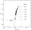 |
Fig. 1 Colour–magnitude diagram for the Hercules dSph galaxy (Adén et al. 2009a). • are RGB stars selected for this study. ° indicate RGB stars too faint for this study and open triangles are horizontal-branch stars. The solid line indicates the isochrone by VandenBerg et al. (2006) with colour transformations by Clem et al. (2004). log g values for different magnitudes as indicated. Note that there are two stars at V0 ~ 18.5 superimposed on each other. |
We estimated the microturbulence, ξt, using the ξt and log g for metal-poor halo stars from Andrievsky et al. (2010). These stars have about the same metallicity and log g as our Hercules RGB stars. A least-square fit to their data, in ξt vs. log g space (Fig. 2), of 35 giant stars yields  (1)We estimated the errors in ξt using the uncertainties for the least-square fit (Eq. (1)) and an uncertainty in log g of 0.3 dex. We find a typical error in ξt of ~0.2 km s-1.
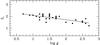 |
Fig. 2 ξt vs. log g for metal-poor giant stars from Andrievsky et al. (2010). The solid line indicates a least-square fit to the data. |
The final stellar parameters used in the abundance analysis are summarised in Table 5.
Photometry and model parameters used in the abundance analysis of the stars.
4. Abundance analysis
Model atmospheres were calculated for the programme stars with the code marcs according to the procedures described in Gustafsson et al. (2008), and using the fundamental parameters in Table 5. Next, a line list was compiled in the wavelength region 6120–6400 Å with spectral lines from neutral and singly ionised atoms from the VALD database (Piskunov et al. 1995; Ryabchikova et al. 1997; Kupka et al. 1999, 2000). Equivalent widths or synthetic spectra were then computed from radiative transfer calculations in spherical geometry in the model atmospheres using the Eqwi/Bsyn codes that share many subroutines and data files with marcs making the analysis largely self-consistent.
For stars with at least two lines measurable, we adopt the mean of the abundances derived from the individual Wλ for each element as the final elemental abundances. For stars more difficult, in terms of identifying absorption lines, the final elemental abundances are determined using a χ2-test (see Sect. 4.2.3)
4.1. Elemental abundance errors
For elements with more than four lines measured, the random errors in the elemental abundance ratios were calculated as ![\begin{equation} \epsilon_{{\rm rand, [X/H]}}=\frac{\sigma_{\rm X}}{\sqrt{N}} \end{equation}](/articles/aa/full_html/2011/01/aa14963-10/aa14963-10-eq61.png) (2)where X is the element, σ is the standard deviation of the abundances derived from the individual Wλ, and N the number of lines for that element. For elements with two to four lines measured, the uncertainty in the measurement of Wλ, ϵWλ, was estimated using the relation in Cayrel (1988). The random errors in the elemental abundances were then estimated using 105 Monte Carlo realisations of Wλ, drawn from within the probability distribution of Wλ given ϵWλ. For each value of Wλ, we recalculate an elemental abundance using the relation log (A) ∝ log (Wλ) where A is the elemental abundance. We note that the probability distribution of log (A) is asymmetric. Thus, we adopt the standard deviation based on the sextiles (which is equivalent to 1σ in the case of a Gaussian distribution) as our final random error. For elements with less than two lines measured we performed a χ2-test between the stellar spectrum and a grid of synthetic spectra, to estimate the random errors in the elemental abundances (see Sects. 4.2 and 4.3). Note that none of the Ca abundances are estimated using more than two lines. Thus, the errors in [Ca/H] are derived using either a χ2-test or by propagating ϵWλ as derived using the relation in Cayrel (1988).
(2)where X is the element, σ is the standard deviation of the abundances derived from the individual Wλ, and N the number of lines for that element. For elements with two to four lines measured, the uncertainty in the measurement of Wλ, ϵWλ, was estimated using the relation in Cayrel (1988). The random errors in the elemental abundances were then estimated using 105 Monte Carlo realisations of Wλ, drawn from within the probability distribution of Wλ given ϵWλ. For each value of Wλ, we recalculate an elemental abundance using the relation log (A) ∝ log (Wλ) where A is the elemental abundance. We note that the probability distribution of log (A) is asymmetric. Thus, we adopt the standard deviation based on the sextiles (which is equivalent to 1σ in the case of a Gaussian distribution) as our final random error. For elements with less than two lines measured we performed a χ2-test between the stellar spectrum and a grid of synthetic spectra, to estimate the random errors in the elemental abundances (see Sects. 4.2 and 4.3). Note that none of the Ca abundances are estimated using more than two lines. Thus, the errors in [Ca/H] are derived using either a χ2-test or by propagating ϵWλ as derived using the relation in Cayrel (1988).
The systematic errors, ϵsys, [X/H] , were estimated from the errors in the stellar parameters (Sect. 3) as follows: two stars were selected randomly, RGB star 40 789 and 42 241. For these two stars, we study the final elemental abundances for several model atmospheres. The model atmospheres were chosen so that we had two values of log g, separated by 0.5 dex, three values of Teff, separated by 100 K, and three values of ξt, separated by 0.2 km s-1. The separation between the Teff and ξt values corresponds to the estimated errors in the parameters (see Sect. 3). The centre value for Teff and ξt corresponds to the values as determined in Sect. 3. Since the error in log g was more difficult to determine (see Sect. 3), we chose a separation in log g of 0.5 dex to make sure that we got an upper limit of the contribution from this stellar parameter. The elemental abundances varies with less than 0.05 dex when the value of log g is separated by 0.5 dex. However, we note that this is based on Fe i lines. Fe ii lines are more sensitive to changes in log g.
Thus, we have 18 model atmospheres for which we determine the final elemental abundances of iron and calcium. The standard deviation of the 18 final elemental abundances, for iron and calcium, is then adopted as ϵsys, [X/H] . We find a typical ϵsys, [X/H] of ~0.12 dex.
The total errors in the elemental abundance ratios were calculated as ![\begin{equation} \epsilon_{{\rm [X/H]}}= \sqrt{\epsilon_{{\rm rand, [X/H]}}^2+\epsilon_{{\rm sys, [X/H]}}^2}. \end{equation}](/articles/aa/full_html/2011/01/aa14963-10/aa14963-10-eq72.png) (3)The final total errors are summarised in Table 6.
(3)The final total errors are summarised in Table 6.
4.2. Iron
The mean [Fe/H] is determined on the scale where log ϵH = 12.00. The solar iron abundance of 7.45 is adopted from Grevesse et al. (2007).
Due to the variation in the S/N, and the number of measurable lines in the spectra, we analyse these stars individually or as groups with spectra of similar quality (Sects. 4.2.1, 4.2.2 and 4.2.3). The result from the analysis is summarised in Table 6.
4.2.1. Highest S/N spectra
RGB star 12 175, with V0 = 18.5, is one of the two brightest RGB stars discovered in the Hercules dSph galaxy. However, due to its low metallicity, only 4 Fe i lines were distinguishable from the continuum in the spectral range covered by our observation. These four iron lines give [Fe/H] = −3.17 ± 0.14. Figure 3b shows the spectrum of 12 175 around two of the four Fe i lines. Close to these two lines there are two additional Fe i lines that we could not measure quantitatively, but that we were able to identify with the help of a synthetic spectrum. The synthetic spectrum shown in Fig. 3b supports the result that this is a very metal-poor star with [Fe/H] = −3.2.
RGB star 42 241 has about the same magnitude and S/N as 12 175. However, due to its higher iron abundance, about four times as many lines were measurable in this spectrum (compare Table 4). We find an [Fe/H] of −2.03 ± 0.14 dex. Additionally, for this star, we were able to measure two Fe ii lines. These lines give an iron abundance of −1.40 ± 0.20 dex. Thus, the [Fe/H] as derived from Fe i lines do not agree within the error bars with [Fe/H] as derived from Fe ii lines. This discrepancy in the determination of the iron abundance could partially be caused by over-ionisation in Fe i. Ivans et al. (2001) argue that over-ionisation could cause an under-estimate of about 0.1 dex for RGB stars if Fe i lines are used.
Figure 3d shows the stellar spectrum of 42 241 around four of the measured Fe i lines. As can be seen, [Fe/H] derived from the Wλ agrees well with a synthetic spectrum with an iron abundance close to the –2 dex value derived from the Wλs.
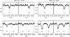 |
Fig. 3 Left panels: portions of stellar spectra around four Fe i b) and two Ca i a) lines for RGB star 12175. • indicate the observed spectrum. The solid line indicates a synthetic spectrum with [Fe/H] = −3.1 and [Ca/H] = −2.8. The dotted lines in a) indicate synthetic spectra with [Ca/H] ± 0.3 relative to the solid-line-synthetic spectrum. Right panels: Portions of stellar spectra around four Fe i d) and two Ca i c) lines for star 42 241. • indicate the observed spectrum. The solid line indicates a synthetic spectrum with [Fe/H] = −2.0 and [Ca/H] = −2.6. |
4.2.2. Low S/N spectra
RGB stars 42 149, 41 743, 42 795, 40 789, 42 096, 40 993 and 12 729 have a lower S/N than 12 175 and 42 241. However, at least two Fe i lines were measurable for each of the stars.
Since the S/N is much lower for these stars, we did the following test to ensure that the [Fe/H] derived from the equivalent widths are reasonable. For each of the stars, we generated a set of synthetic spectra with five different [Fe/H] values, separated by 0.2 dex, centred on the [Fe/H] derived from the equivalent widths. A plot of the stellar spectrum, with the synthetic spectra over-plotted, enabled us to verify that the [Fe/H] derived from the Wλs is a good estimate of the iron abundance of the star. We found that none of the stellar spectra deviated significantly from a synthetic spectrum with a similar [Fe/H] abundance.
Figure 4 shows an example, for 41 743. As can be seen, an [Fe/H] of ~ −2.4 dex is a reasonable estimate of the iron abundance for this star.
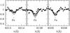 |
Fig. 4 Portions of stellar spectra around three Fe i lines for RGB star 41 743. • indicate the observed spectra. The solid lines indicate synthetic spectra with [Fe/H] from −2.85 to −2.05 dex, top to bottom, separated by 0.2 dex each. |
4.2.3. Difficult spectra
RGB stars 41 460 and 42 324 have low S/N (21 and 13, respectively) and are very metal-poor. Thus, it was difficult to identify the Fe i absorption lines in the spectra. However, we did see faint absorption signatures but the low S/N made it virtually impossible to measure the lines. Instead, we performed a χ2-test between the observed spectrum and a grid of synthetic spectra with 17 different [Fe/H] values, separated by 0.05 dex. Each synthetic spectrum yields a χ2 value, and the best fit is found when χ2 is minimised ( ). We used a width of 3σ, which covers about 99.7 per cent of the absorption feature, for each iron line in the line list (see Table 4). We investigated the sensitivity of the χ2-test region by varying it between 2σ and 4σ and found that it had negligible impact on the result. The continuum for each line was adjusted, as the average of the signal on each side of the absorption feature over 0.6 Å, to accommodate for the local deviations from the continuum normalisation in Sect. 2.3. The error for each pixel in the observed spectrum was approximated by the variance in the spectrum. The distribution enclosed by
  corresponds to 1σ for a normal distribution (Press et al. 1992). We used this as the measurement error.
4.3. Calcium
The mean [Ca/H] is determined on the scale where log ϵH = 12.00 The solar calcium abundance of 6.34 is adopted from Asplund et al. (2009). There are two Ca i lines, at 6122.22 Å and 6162.17 Å in the wavelength region covered by our spectra, that were possible to measure in the majority of the stars. The results from the analysis are summarised in Table 6. Individual stars are, in similar manner as done for Fe, discussed in the following sections.
4.3.1. Highest S/N spectra
For RGB star 12 175 both Ca i lines were measured and they give [Ca/H] = −2.9 ± 0.1. Figure 3a shows the stellar spectrum around the Ca i lines. As can be seen, [Ca/H] as measured from the Wλ agree well with a synthetic spectrum with similar [Ca/H]. Additionally, Fig. 3a shows an example of two synthetic spectra with [Ca/H] ± 0.3.
For RGB star 42 241 we find a [Ca/H] of −2.5 ± 0.2. This is significantly higher than [Ca/H] for RGB star 12 175. Figure 3c shows the stellar spectrum of 42 241 around the two Ca i lines. As can be seen, [Ca/H] as derived from the Wλ agree well with a synthetic spectrum with a similar abundance.
4.3.2. Low S/N spectra
RGB stars 42 149, 41 743, 40 789, 42 096 and 42 324 have a lower S/N than RGB stars 12 175 and 42 241. However, both of the Ca i lines were measurable in all four stars.
Since the S/N is lower we repeated the same test done for the iron abundance analysis (compare Sect. 4.2.2), generating a grid of synthetic spectra for each star, to see if the [Ca/H] as derived from the Wλ were reasonable. We found that the synthetic spectrum of RGB star 40 789, in comparison with the observed spectrum, indicates that the [Ca/H] determined from the measurements of the Wλ was slightly, about 0.1 dex, over-estimated. Thus, we estimated the Ca i abundance for RGB star 40 789 using the same method as for the spectra identified as difficult for the measurement of the Fe i lines (see Sect. 4.2.3). For all other stars in this category, the abundances from the measured Wλ and those from the χ2-comparison of synthetic spectra showed good agreement.
4.3.3. Difficult spectra
For RGB star 42 795, 41 460, and 40 993 only one or none of the Ca i lines were measurable. However we did see a general decrease in the continuum at the wavelengths for the Ca i lines indicating the presence of Ca in the atmospheres of these metal-poor stars. Thus, we estimated the Ca i abundance using the same method as for the spectra identified as difficult for the measurement of the Fe i lines (see Sect. 4.2.3). The results from the analysis are summarised in Table 6.
We were not able to identify any Ca i absorption features for RGB star 12 729. Thus, [Ca/H] remains unknown for this star.
Derived elemental abundances for the RGB stars in the Hercules dSph galaxy.
5. A comparison with abundances determined in other studies
5.1. A comparison with a high S/N RGB star
Lind et al. (2009) obtained high S/N spectroscopy of several bright RGB stars in the Milky Way. They used the same instrument and grating (GIRAFFE/HR13) as in this study. Through private communication they provided us with a spectrum of one of their bright targets, star 17691, that has a S/N of about 300. We measured the Wλ for the lines in Table 4 and performed an abundance analysis for this star as described in Sects. 2.3 and 4. The stellar parameters was adopted from Lind et al. (2009). We find an Fe abundance that is 0.01 dex more metal poor, and a Ca abundance 0.04 dex lower than given in Lind et al. (2009). Thus, our determinations of the abundances of Ca and Fe in star 17691 are in agreement with Lind et al. (2009). Additionally, we find that none of the elemental abundances as derived from individual measurements of the Wλ deviate significantly. This suggests that the effect of atomic parameters should not contribute to our elemental abundance errors.
5.2. A comparison with earlier spectroscopic results
Koch et al. (2008b) obtained high resolution spectroscopy (R ~ 20 000), with similar S/N and resolution as in this study, of two stars in the Hercules dSph galaxy, Her-2 and Her-3. These stars correspond to our RGB stars 42 241 and 41 082. However, RGB star 41 082 was discarded from our sample (see Sect. 4). Koch et al. (2008b) find [Fe/H] = −2.02 ± 0.20 and [Ca/Fe] = −0.13 ± 0.05 for RGB star 42 241. Note, however, that Koch et al. (2008b) measured Wλ values of lines over a broader wavelength range from 5500–8900 Å. Our estimates of [Fe/H] are in very good agreement, but [Ca/Fe] as derived by Koch et al. (2008b) is 0.4 dex higher.
Equivalent width measurements for RGB star 42 241/Her-2.
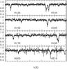 |
Fig. 5 A comparison between our spectrum and the spectrum from Koch et al. (2008b) , in the region where they overlap, for RGB star 42 241. • indicate our stellar spectrum. The solid line indicates the spectrum from Koch et al. (2008b). |
Figure 5 shows our spectrum and the spectrum from Koch et al. (2008b) for RGB star 42 241. In Table 7 we provide a comparison between Wλs as measured from our observed spectrum, and Wλs as measured by us from the spectrum obtained by Koch et al. (2008b). We note that, for the Ca i lines, the spectrum from Koch et al. (2008b) has deeper absorption. However, the overall absorption for the Fe i and blended lines are in good agreement, except for one weak Fe i line at λ = 6200.31 Å that is more prominent in our observed spectrum. We note that the S/N at this line in the spectrum from Koch et al. (2008b) is low, making it difficult to distinguish such a weak line in the spectrum. There is a much brighter star, SDSS J163056.63+124737.5, located only ~12 arcsec from 42 241. Thus, we investigate the possibility that the fibre allocated for 42241 has collected a significant amount of flux from SDSS J163056.63+124737.5. SDSS J163056.63+124737.5 is 6.7 mag brighter in the SDDS r-filter, which is centred on our wavelength region of interest. The seeing for our observations was ~1 arcsec. Based on this, we constructed a model of two Gaussian flux distributions with a full-width half-maximum of 1.5 arcsec and magnitudes that represent the brightness of the stars. We found that the amount of flux from SDSS J163056.63+124737.5 at the position of the fibre is negligible. A similar investigation was carried out for the spectrum obtained by Koch et al. (2008b), yielding the same conclusion. Thus, the origin of this discrepancy can not be due to a contamination by light from this nearby star. A more thorough investigation than this goes beyond the scope of this study. However, one could speculate that there is an unresolved binary present that was overlapped in one observation and out of phase in the other observation, or that it may be due to some differences in the reduction procedure.
Kirby et al. (2008b) studied 20 stars in the direction of the Hercules dSph galaxy. Their metallicities are based on a recently developed automated spectrum synthesis method that takes the information in the whole spectrum into account (Kirby et al. 2008a). The method was originally developed for globular clusters in the Milky Way and was then applied to ultra-faint dSph galaxies in Kirby et al. (2008b). We have 7 stars in common between our samples. Figure 6b shows the difference between our respective determinations of [Fe/H]. We find that our [Fe/H] is on average 0.07 dex more metal-rich, with a scatter of 0.09 dex. In conclusion, the agreement between the [Fe/H] determinations is very good.
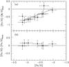 |
Fig. 6 a) A comparison between our [Fe/H] and [M/H] from Adén et al. (2009a) ( [M/H] Phot). The error-bars represent the error in [Fe/H] − [M/H] Phot and [Fe/H], respectively. b) A comparison between our [Fe/H] and [Fe/H] from Kirby et al. (2008b) ( [Fe/H] Kirby). The error-bars represent the error in [Fe/H] − [Fe/H] Kirby and [Fe/H], respectively. |
5.3. A comparison with earlier photometric results
In a previous study of the Hercules dSph galaxy (Adén et al. 2009a) we estimated [Fe/H] using the Strömgren m1 index using the calibration from Calamida et al. (2007). Figure 6a shows a comparison between the photometric [Fe/H] as estimated in Adén et al. (2009a), [M/H] phot, and [Fe/H] as determined from high-resolution spectroscopy in this study. We note that there is a strong trend such that [M/H] appears to be over-estimated in Adén et al. (2009a) for metal-poor stars.
5.4. A new metallicity calibration for Strömgren photometry for metal-poor red giant stars
Given the excellent agreement between all three spectroscopic studies it must be concluded that the metallicity calibration by Calamida et al. (2007) over-estimates the metallicity for very metal-poor stars. This result is expected, since the calibration by Calamida et al. (2007) is valid only for [Fe/H] > −2.4 This is an unfortunate situation since the photometry allows us in principle to determine the metallicity of RGB stars with good accuracy also for the fainter stars (compare errors in Adén et al. 2009a) and thus allowing the study of much more complete stellar samples in the ultra-faint dSph galaxies.
Here we present an attempt to deal with the situation. So far this is a very simplistic relation and only formally valid for stars with 0.02 < m1,0 < 0.40, −3.29 < [Fe/H] < 1.58 and 1.15 < (v − y)0 < 2.18.
We have collected all spectroscopic [Fe/H] derived from high-resolution spectra available for stars in Draco (Cohen & Huang 2009; Shetrone et al. 2001), Sextans (Shetrone et al. 2001), UMaII (Frebel et al. 2010b) and Hercules (this study), and combined these data with our own Strömgren photometry where available. Figure 7a shows the spectroscopic [Fe/H] as a function of m1,0 for the stars. A least-squares fit yields
![\begin{equation} \label{eq_phot_new} {\rm [M/H]_{phot,\,new}}=4.51(\pm 0.41) \, m_{1,0} - 3.38(\pm 0.10). \end{equation}](/articles/aa/full_html/2011/01/aa14963-10/aa14963-10-eq145.png) (4)Figures 7b,c show [M/H] phot, new − [Fe/H] as a function of m1,0 and (v − y)0, respectively. No strong trends are seen. For comparison Fig. 7d shows [M/H] CA07 − [Fe/H] vs. (v − y)0, where [M/H] CA07 is [Fe/H] as determined using the calibration in Calamida et al. (2007). Here we can note a significant difference of both metallicity scales such that [M/H] CA07 > [Fe/H] spec. Taking into account the uncertainties of the least-squares fit and the correlation between the fitting parameters (Eq. (4)), and the error in m1,0 from Adén et al. (2009a) we find a typical error in [M/H] phot, new of 0.17 dex.
(4)Figures 7b,c show [M/H] phot, new − [Fe/H] as a function of m1,0 and (v − y)0, respectively. No strong trends are seen. For comparison Fig. 7d shows [M/H] CA07 − [Fe/H] vs. (v − y)0, where [M/H] CA07 is [Fe/H] as determined using the calibration in Calamida et al. (2007). Here we can note a significant difference of both metallicity scales such that [M/H] CA07 > [Fe/H] spec. Taking into account the uncertainties of the least-squares fit and the correlation between the fitting parameters (Eq. (4)), and the error in m1,0 from Adén et al. (2009a) we find a typical error in [M/H] phot, new of 0.17 dex.
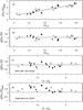 |
Fig. 7 a) Spectroscopic [Fe/H] vs. m1,0 for Draco (• and °), Sextans (open stars), UMaII (filled triangles) and Hercules (filled squares). b), [M/H] phot, new − [Fe/H] vs. m1,0 using Eq. (4) to derive [M/H]. c), [M/H] phot, new − [Fe/H] vs. (v − y)0 using Eq. (4) to derive [M/H]. d) [M/H] CA07 − [Fe/H] vs. (v − y)0 using the calibration by Calamida et al. (2007) to derive [M/H]. |
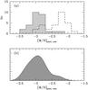 |
Fig. 8 a) Metallicity histogram for RGB stars in the Hercules dSph galaxy. The shaded histogram shows the distribution of [M/H] phot, new. For comparison, the dashed histogram shows the distribution of [M/H] phot (Adén et al. 2009a). b) Corresponding error-weighted metallicity distribution. |
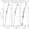 |
Fig. 9 a) and b) Colour–magnitude diagrams for RGB stars with high–resolution spectroscopy of the Hercules dSph galaxy. • indicate RGB stars more metal-poor than [Fe/H] = −2.7. ° represents RGB stars more metal-rich than, or equal to, [Fe/H] = −2.7. The filled square indicates the most metal-rich RGB star at [Fe/H] = −2.0. The solid and dashed lines represent isochrones with [Fe/H] = −2.31 and −2.14 dex, respectively, by VandenBerg et al. (2006) with colour transformations by Clem et al. (2004). c) Colour–magnitude diagram for the RGB stars in Adén et al. (2009a) with [M/H] phot, new as determined in Sect. 5.4. • indicate RGB stars more metal-poor than [M/H] = −2.8. ° indicate RGB stars more metal-rich than [M/H] = −2.8. Isochrones as in b). The error bars on the right hand side in each figure represent the typical error in (v − y)0. |
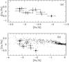 |
Fig. 10 a) [Ca/Fe] as a function of [Fe/H]. Filled triangle and filled square indicate our two brightest RGB stars, RGB stars 12 175 and 42 241, respectively. The error-bars represent the error in [Ca/Fe] and [Fe/H], respectively. b) Same as a) but with a compilation of the Milky Way disk and halo stars abundances from Venn et al. (2004), as indicated by small dots. |
6. Results and discussion
6.1. Iron abundance and ages for the RGB stars in Hercules
The RGB stars analysed in this paper span a large range of iron abundances, from about –3.2 dex to –2 dex, indicating an extended period of chemical enrichment. It is somewhat fortuitous that the two brightest stars in our sample, RGB stars 12 175 and 42 241, bracket the full range of metallicities. Thus, there is no doubt that the range of metallicities derived from high-resolution spectroscopy is real.
In Sect. 5.4 we provide a new Strömgren metallicity calibration. This calibration is valid for stars with 0.02 < m1,0 < 0.40 and −3.29 < [Fe/H] < 1.58. Two of the 28 RGB stars from Adén et al. (2009a) have an m1,0 less than the range for which the new metallicity calibration is valid. However, with an m1,0 of 0.01, these stars are included in the sample as a slight extrapolation. In Fig. 8a we show the resulting histogram of [M/H] phot, new for all the 28 RGB stars identified in (Adén et al. 2009a). The bin size of 0.2 dex represents the typical error in [M/H] phot, new (see Sect. 5.4). Figure 8b shows the corresponding error-weighted metallicity distribution. For this plot, each stars was assigned a Gaussian distribution with a mean of [M/H] phot, new and a dispersion equal to the typical error in [M/H] phot, new (0.17 dex). The Gaussians, one for each star, were then added to create the metallicity distribution function. We note that the distribution of [M/H] phot, new is shifted towards lower metallicities when the new calibration is applied, and that there is an abundance spread in the metallicity distribution for the RGB stars of at least 1.0 dex. Additionally, we note a more concentrated distribution.
Figure 9a,b show V0 vs. (v − y)0 for the stars with [Fe/H] derived from high resolution spectroscopy. Additionally, in these plots, we show two isochrones with [Fe/H] = −2.31 (most metal-poor isochrone available) and −2.14 dex. As can be seen, the isochrones of a given metallicity become redder with increasing age. Since the isochrone with [Fe/H] = −2.31 is too metal-rich, compared to [Fe/H] as derived from the spectroscopy, an even more metal-poor isochrone at the age of 8 Gyr would be even bluer, excluding an age of about 10 Gyr or younger. At an age of 14 Gyr, the isochrone with [Fe/H] = −2.31 is slightly redder than most of the stars more metal-poor than [Fe/H] = −2.7. Hence a more metal-poor isochrone would presumably represent the locus of these stars very well, arguing for an age older than about 10 Gyr for the Hercules dSph galaxy.
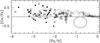 |
Fig. 11 A comparison of [Ca/Fe] as a function of [Fe/H] for stars in several dSph galaxies. • indicate Hercules (this study). Filled squares represent the ultra-faint dSph galaxies Ursa Major II, Coma Berenices, Boötes I and Leo IV (Feltzing et al. 2009; Frebel et al. 2010b; Norris et al. 2010; Simon et al. 2010). Open squares represent the classical dSph galaxies Draco, Sextans, Ursa Minor, Fornax, Carina and Sculptor (Shetrone et al. 2001, 2003; Sadakane et al. 2004; Koch et al. 2008a; Cohen & Huang 2009; Aoki et al. 2009; Frebel et al. 2010a). The solid ellipses outline RGB stars in the classical dSph galaxy Fornax from Letarte et al. (2007). |
Figure 9c shows V0 vs. (v − y)0 for all the 28 RGB stars identified in (Adén et al. 2009a).
6.2. [Ca/Fe]
Figure 10 shows [Ca/Fe] as a function of [Fe/H]. We find a trend such that [Ca/Fe] is higher for more metal-poor stars, and lower for more metal-rich stars. Fortuitously, the most metal-rich and the most metal-poor star in the sample are both bright and have spectra with high S/N (see discussion in Sect. 4 and also Table 2). Thus we can be certain that the trend actually has this shape and we are not misinterpreting spectra of lower quality.
The production of alpha (α)-elements, such as Ca, Si, Ti, Mg, and O, is correlated with the end stage of massive stars. Mg and O are created during the hydrostatic He burning in massive stars, and Si, Ca, and Ti are primarily produced during core-collapse supernovae (Woosley & Weaver 1995). On the other hand, less massive stars are able to produce significant amounts of Fe in SNe Ia. Thus, the ratio of α-elements to iron is used to trace the time scale of the star formation in a stellar system. If the star formation rate is high, then the gas will be able to reach a higher [Fe/H] before the first SNe Ia occur. This can be observed in a plot of [Ca/Fe] vs. [Fe/H] as a “knee”, where [Ca/Fe] decrease as [Fe/H] increase (McWilliam 1997). The fraction of stars at [Fe/H] less than the “knee” gives information on the star formation timescale.
The observed continuous downward trend, without a “knee”, for [Ca/Fe] vs. [Fe/H] in Hercules can thus be interpreted as a brief initial burst of short-lived SNe II that enhanced the production of α-elements. Since there are no stars at [Fe/H] less than the “knee”, the star formation rate was very low. The subsequent continuous decline would be expected if contributions from long-lived SNe Ia were the dominant factor, decreasing [α/Fe] while increasing [Fe/H]. This means that essentially no massive stars formed after the initial burst. Additionally, we interpret the relatively short range in [Fe/H] (no stars with [Fe/H] > −2 are seen in our sample) as a tentative evidence for a short duration of this low-efficiency star formation (for a discussion of continuous and bursty star formation histories and the role of SNe Ia see, e.g., Gilmore & Wyse 1991; Matteucci 2009). The classical dSph galaxies, such as Carina, Sculptor and Fornax, also show these types of trends for the α-elements (e.g., Venn et al. 2004; Koch et al. 2008a; Tolstoy et al. 2009; Kirby et al. 2009). However, these dSph galaxies are more metal-rich and more massive than, e.g., Hercules. Only a few other ultra-faint dSphs have chemical element abundances published for only a handful of stars each.
Frebel et al. (2010b), Feltzing et al. (2009), Norris et al. (2010) and Simon et al. (2010) studied Coma Berenices, Ursa Major II, Boötes I, and Leo IV, all recently discovered ultra-faint and metal-poor systems. Figure 11 summarises our data and their data. Additionally, recent studies have analysed very metal-poor stars in the classical systems Draco, Sextans and Sculptor (Cohen & Huang 2009; Aoki et al. 2009; Frebel et al. 2010a). We add these new data to the plot in addition to the abundances from other studies of Fornax, Carina, Sculptor, Sextans, Ursa Minor and Draco (Shetrone et al. 2001, 2003; Sadakane et al. 2004; Letarte et al. 2007; Koch et al. 2008a).
Overall, there is a faster declining [Ca/Fe] with [Fe/H] for the dSph galaxies as compared with the halo stars in the solar neighbourhood (from the compilation by Venn et al. 2004, including data from Fulbright (2002, 2000); Stephens & Boesgaard (2002); Bensby et al. (2003); Nissen & Schuster (1997); Hanson et al. (1998); Prochaska et al. (2000); Reddy et al. (2003); Edvardsson et al. (1993); McWilliam (1998); McWilliam et al. (1995); Johnson (2002); Burris et al. (2000); Ivans et al. (2003); Ryan et al. (1996); Gratton & Sneden (1991, 1994, 1988)). Thus, for example, the trend seen from our data in Hercules is the same as the overall trend seen for Draco. This is interesting and could be interpreted as that the Fe contribution from SNe Ia were the dominant factor for both Hercules and Draco. However, since Draco has many more stars with [Fe/H] > −2 it must have had a more integrated star formation than the Hercules dSph galaxy, as may be expected given its higher baryon content.
7. Conclusions
We have studied confirmed RGB stars in the ultra-faint Hercules dSph galaxy with FLAMES high-resolution spectroscopy. Abundances were determined by solving the radiative transfer calculations using the codes Eqwi/Bsyn in marcs model atmospheres.
We find that the RGB stars of the Hercules dSph galaxy included in this study are more metal-poor than estimated in Adén et al. (2009a), however in good agreement with Kirby et al. (2008b), with a metallicity spread of at least 1 dex. Based on the position of the RGB stars in colour–magnitude diagrams, in comparison with isochrones, we conclude that there is no clear indication of a population younger than about 10 Gyr.
Additionally, we provide a first attempt at a new metallicity calibration for Strömgren photometry based on high-resolution spectroscopy for several dSph galaxies. With this new calibration, we find several RGB stars in the Hercules dSph galaxy that are more metal-poor than [Fe/H] = −3.0 dex.
Finally, we have determined the [Ca/Fe] for the RGB stars in this study. We found a trend such that [Ca/Fe] is higher for more metal-poor stars, and lower for more metal-rich stars. This trend is supported by our two brightest stars in the sample and is interpreted as a brief initial burst of SNe II during a very low star formation rate, followed by the enrichment of [Fe/H] by SNe Ia.
Acknowledgments
We acknowledge Karin Lind for providing us with a spectrum of one of their RGB stars. S.F. is a Royal Swedish Academy of Sciences Research Fellow supported by a grant from the Knut and Alice Wallenberg Foundation. K.E. is gratefully acknowledging support from the Swedish research council. M.I.W. is supported by a Royal Society University Research Fellowship. AK acknowledges support by an STFC postdoctoral fellowship.
References
- Adén, D., Feltzing, S., Koch, A., et al. 2009a, A&A, 506, 1147 [NASA ADS] [CrossRef] [EDP Sciences] [Google Scholar]
- Adén, D., Wilkinson, M. I., Read, J. I., et al. 2009b, ApJ, 706, L150 [NASA ADS] [CrossRef] [Google Scholar]
- Alonso, A., Arribas, S., & Martínez-Roger, C. 1999, A&AS, 140, 261 [NASA ADS] [CrossRef] [EDP Sciences] [Google Scholar]
- Andrievsky, S. M., Spite, M., Korotin, S. A., et al. 2010, A&A, 509, A88 [NASA ADS] [CrossRef] [EDP Sciences] [Google Scholar]
- Aoki, W., Arimoto, N., Sadakane, K., et al. 2009, A&A, 502, 569 [NASA ADS] [CrossRef] [EDP Sciences] [Google Scholar]
- Asplund, M., Grevesse, N., Sauval, A. J., & Scott, P. 2009, ARA&A, 47, 481 [NASA ADS] [CrossRef] [Google Scholar]
- Belokurov, V., Zucker, D. B., Evans, N. W., et al. 2007, ApJ, 654, 897 [NASA ADS] [CrossRef] [Google Scholar]
- Bensby, T., Feltzing, S., & Lundström, I. 2003, A&A, 410, 527 [NASA ADS] [CrossRef] [EDP Sciences] [Google Scholar]
- Blecha, A., Cayatte, V., North, P., Royer, F., & Simond, G. 2000, in Optical and IR Telescope Instrumentation and Detectors, ed. M. Iye, & A. F. Moorwood, SPIE Conf., 4008, 467 [Google Scholar]
- Burris, D. L., Pilachowski, C. A., Armandroff, T. E., et al. 2000, ApJ, 544, 302 [NASA ADS] [CrossRef] [Google Scholar]
- Calamida, A., Bono, G., Stetson, P. B., et al. 2007, ApJ, 670, 400 [NASA ADS] [CrossRef] [Google Scholar]
- Calamida, A., Bono, G., Stetson, P. B., et al. 2009, ApJ, 706, 1277 [NASA ADS] [CrossRef] [Google Scholar]
- Cayrel, R. 1988, in The Impact of Very High S/N Spectroscopy on Stellar Physics, ed. G. Cayrel de Strobel & M. Spite, IAU Symp., 132, 345 [Google Scholar]
- Clem, J. L., VandenBerg, D. A., Grundahl, F., & Bell, R. A. 2004, AJ, 127, 1227 [NASA ADS] [CrossRef] [Google Scholar]
- Cohen, J. G., & Huang, W. 2009, ApJ, 701, 1053 [NASA ADS] [CrossRef] [Google Scholar]
- Dotter, A., Chaboyer, B., Jevremović, D., et al. 2008, ApJS, 178, 89 [NASA ADS] [CrossRef] [Google Scholar]
- Edvardsson, B., Andersen, J., Gustafsson, B., et al. 1993, A&A, 275, 101 [NASA ADS] [Google Scholar]
- Feltzing, S., Eriksson, K., Kleyna, J., & Wilkinson, M. I. 2009, A&A, 508, L1 [NASA ADS] [CrossRef] [EDP Sciences] [Google Scholar]
- Frebel, A., Kirby, E. N., & Simon, J. D. 2010a, Nature, 464, 72 [NASA ADS] [CrossRef] [Google Scholar]
- Frebel, A., Simon, J. D., Geha, M., & Willman, B. 2010b, ApJ, 708, 560 [NASA ADS] [CrossRef] [Google Scholar]
- Fulbright, J. P. 2000, AJ, 120, 1841 [NASA ADS] [CrossRef] [Google Scholar]
- Fulbright, J. P. 2002, AJ, 123, 404 [NASA ADS] [CrossRef] [Google Scholar]
- Geisler, D., Wallerstein, G., Smith, V. V., & Casetti-Dinescu, D. I. 2007, PASP, 119, 939 [NASA ADS] [CrossRef] [Google Scholar]
- Gilmore, G., & Wyse, R. F. G. 1991, ApJ, 367, L55 [NASA ADS] [CrossRef] [Google Scholar]
- Gratton, R. G., & Sneden, C. 1988, A&A, 204, 193 [NASA ADS] [Google Scholar]
- Gratton, R. G., & Sneden, C. 1991, A&A, 241, 501 [NASA ADS] [Google Scholar]
- Gratton, R. G., & Sneden, C. 1994, A&A, 287, 927 [NASA ADS] [Google Scholar]
- Grebel, E. K., & Gallagher, III, J. S. 2004, ApJ, 610, L89 [NASA ADS] [CrossRef] [Google Scholar]
- Grevesse, N., Asplund, M., & Sauval, A. J. 2007, Space Sci. Rev., 130, 105 [Google Scholar]
- Gustafsson, B., Edvardsson, B., Eriksson, K., et al. 2008, A&A, 486, 951 [NASA ADS] [CrossRef] [EDP Sciences] [Google Scholar]
- Hanson, R. B., Sneden, C., Kraft, R. P., & Fulbright, J. 1998, AJ, 116, 1286 [NASA ADS] [CrossRef] [Google Scholar]
- Helmi, A., Irwin, M. J., Tolstoy, E., et al. 2006, ApJ, 651, L121 [NASA ADS] [CrossRef] [Google Scholar]
- Ivans, I. I., Kraft, R. P., Sneden, C., et al. 2001, AJ, 122, 1438 [NASA ADS] [CrossRef] [Google Scholar]
- Ivans, I. I., Sneden, C., James, C. R., et al. 2003, ApJ, 592, 906 [NASA ADS] [CrossRef] [Google Scholar]
- Johnson, J. A. 2002, ApJS, 139, 219 [NASA ADS] [CrossRef] [Google Scholar]
- Kirby, E. N., Guhathakurta, P., & Sneden, C. 2008a, ApJ, 682, 1217 [NASA ADS] [CrossRef] [Google Scholar]
- Kirby, E. N., Simon, J. D., Geha, M., Guhathakurta, P., & Frebel, A. 2008b, ApJ, 685, L43 [NASA ADS] [CrossRef] [Google Scholar]
- Kirby, E. N., Guhathakurta, P., Bolte, M., Sneden, C., & Geha, M. C. 2009, ApJ, 705, 328 [NASA ADS] [CrossRef] [Google Scholar]
- Koch, A. 2009, Astron. Nach., 330, 675 [NASA ADS] [CrossRef] [Google Scholar]
- Koch, A., Grebel, E. K., Wyse, R. F. G., et al. 2006, AJ, 131, 895 [NASA ADS] [CrossRef] [Google Scholar]
- Koch, A., Grebel, E. K., Gilmore, G. F., et al. 2008a, AJ, 135, 1580 [NASA ADS] [CrossRef] [Google Scholar]
- Koch, A., McWilliam, A., Grebel, E. K., Zucker, D. B., & Belokurov, V. 2008b, ApJ, 688, L13 [NASA ADS] [CrossRef] [Google Scholar]
- Kupka, F., Piskunov, N., Ryabchikova, T. A., Stempels, H. C., & Weiss, W. W. 1999, A&AS, 138, 119 [NASA ADS] [CrossRef] [EDP Sciences] [MathSciNet] [PubMed] [Google Scholar]
- Kupka, F. G., Ryabchikova, T. A., Piskunov, N. E., Stempels, H. C., & Weiss, W. W. 2000, Baltic Astron., 9, 590 [Google Scholar]
- Letarte, B., Hill, V., & Tolstoy, E. 2007, in EAS Publications Series, ed. E. Emsellem, H. Wozniak, G. Massacrier, J.-F. Gonzalez, J. Devriendt, & N. Champavert, EAS Publ. Ser., 24, 33 [Google Scholar]
- Lind, K., Primas, F., Charbonnel, C., Grundahl, F., & Asplund, M. 2009, A&A, 503, 545 [NASA ADS] [CrossRef] [EDP Sciences] [MathSciNet] [Google Scholar]
- Martin, N. F., de Jong, J. T. A., & Rix, H. 2008, ApJ, 684, 1075 [NASA ADS] [CrossRef] [Google Scholar]
- Matteucci, F. 2009, Mem. Soc. Astron. Ital., 80, 83 [NASA ADS] [Google Scholar]
- McWilliam, A. 1997, ARA&A, 35, 503 [NASA ADS] [CrossRef] [Google Scholar]
- McWilliam, A. 1998, AJ, 115, 1640 [NASA ADS] [CrossRef] [Google Scholar]
- McWilliam, A., Preston, G. W., Sneden, C., & Shectman, S. 1995, AJ, 109, 2736 [NASA ADS] [CrossRef] [Google Scholar]
- Nissen, P. E., & Schuster, W. J. 1997, A&A, 326, 751 [NASA ADS] [Google Scholar]
- Norris, J. E., Yong, D., Gilmore, G., & Wyse, R. F. G. 2010, ApJ, 711, 350 [NASA ADS] [CrossRef] [Google Scholar]
- Pasquini, L., Avila, G., Blecha, A., et al. 2002, The Messenger, 110, 1 [NASA ADS] [Google Scholar]
- Piskunov, N. E., Kupka, F., Ryabchikova, T. A., Weiss, W. W., & Jeffery, C. S. 1995, A&AS, 112, 525 [Google Scholar]
- Press, W. H., Teukolsky, S. A., Vetterling, W. T., & Flannery, B. P. 1992, Numerical recipes in FORTRAN. The art of scientific computing, ed. W. H., Press, S. A., Teukolsky, W. T., Vetterling, & B. P., Flannery [Google Scholar]
- Prochaska, J. X., Naumov, S. O., Carney, B. W., McWilliam, A., & Wolfe, A. M. 2000, AJ, 120, 2513 [NASA ADS] [CrossRef] [Google Scholar]
- Reddy, B. E., Tomkin, J., Lambert, D. L., & Allen de Prieto, C. 2003, MNRAS, 340, 304 [NASA ADS] [CrossRef] [Google Scholar]
- Ryabchikova, T. A., Piskunov, N. E., Kupka, F., & Weiss, W. W. 1997, Baltic Astron., 6, 244 [Google Scholar]
- Ryan, S. G., Norris, J. E., & Beers, T. C. 1996, ApJ, 471, 254 [NASA ADS] [CrossRef] [Google Scholar]
- Sadakane, K., Arimoto, N., Ikuta, C., et al. 2004, PASJ, 56, 1041 [NASA ADS] [Google Scholar]
- Schlegel, D. J., Finkbeiner, D. P., & Davis, M. 1998, ApJ, 500, 525 [NASA ADS] [CrossRef] [Google Scholar]
- Schörck, T., Christlieb, N., Cohen, J. G., et al. 2009, A&A, 507, 817 [NASA ADS] [CrossRef] [EDP Sciences] [Google Scholar]
- Shetrone, M. D., Côté, P., & Sargent, W. L. W. 2001, ApJ, 548, 592 [NASA ADS] [CrossRef] [Google Scholar]
- Shetrone, M., Venn, K. A., Tolstoy, E., et al. 2003, AJ, 125, 684 [NASA ADS] [CrossRef] [Google Scholar]
- Simon, J. D. & Geha, M. 2007, ApJ, 670, 313 [NASA ADS] [CrossRef] [Google Scholar]
- Simon, J. D., Frebel, A., McWilliam, A., Kirby, E. N., & Thompson, I. B. 2010, ApJ, 716, 446 [NASA ADS] [CrossRef] [Google Scholar]
- Starkenburg, E., Hill, V., Tolstoy, E., et al. 2010, A&A, 513, A34 [NASA ADS] [CrossRef] [EDP Sciences] [Google Scholar]
- Stephens, A., & Boesgaard, A. M. 2002, AJ, 123, 1647 [NASA ADS] [CrossRef] [Google Scholar]
- Tollerud, E. J., Bullock, J. S., Strigari, L. E., & Willman, B. 2008, ApJ, 688, 277 [NASA ADS] [CrossRef] [Google Scholar]
- Tolstoy, E., Hill, V., & Tosi, M. 2009, ARA&A, 47, 371 [NASA ADS] [CrossRef] [Google Scholar]
- VandenBerg, D. A., Bergbusch, P. A., & Dowler, P. D. 2006, ApJS, 162, 375 [NASA ADS] [CrossRef] [MathSciNet] [Google Scholar]
- Venn, K. A., Irwin, M., Shetrone, M. D., et al. 2004, AJ, 128, 1177 [NASA ADS] [CrossRef] [Google Scholar]
- Walker, M. G., Mateo, M., Olszewski, E. W., et al. 2009, ApJ, 704, 1274 [NASA ADS] [CrossRef] [Google Scholar]
- Woosley, S. E., & Weaver, T. A. 1995, ApJS, 101, 181 [NASA ADS] [CrossRef] [Google Scholar]
- Zucker, D. B., Belokurov, V., Evans, N. W., et al. 2006, ApJ, 650, L41 [NASA ADS] [CrossRef] [Google Scholar]
All Tables
All Figures
|
Fig. 1 Colour–magnitude diagram for the Hercules dSph galaxy (Adén et al. 2009a). • are RGB stars selected for this study. ° indicate RGB stars too faint for this study and open triangles are horizontal-branch stars. The solid line indicates the isochrone by VandenBerg et al. (2006) with colour transformations by Clem et al. (2004). log g values for different magnitudes as indicated. Note that there are two stars at V0 ~ 18.5 superimposed on each other. |
| In the text | |
|
Fig. 2 ξt vs. log g for metal-poor giant stars from Andrievsky et al. (2010). The solid line indicates a least-square fit to the data. |
| In the text | |
|
Fig. 3 Left panels: portions of stellar spectra around four Fe i b) and two Ca i a) lines for RGB star 12175. • indicate the observed spectrum. The solid line indicates a synthetic spectrum with [Fe/H] = −3.1 and [Ca/H] = −2.8. The dotted lines in a) indicate synthetic spectra with [Ca/H] ± 0.3 relative to the solid-line-synthetic spectrum. Right panels: Portions of stellar spectra around four Fe i d) and two Ca i c) lines for star 42 241. • indicate the observed spectrum. The solid line indicates a synthetic spectrum with [Fe/H] = −2.0 and [Ca/H] = −2.6. |
| In the text | |
|
Fig. 4 Portions of stellar spectra around three Fe i lines for RGB star 41 743. • indicate the observed spectra. The solid lines indicate synthetic spectra with [Fe/H] from −2.85 to −2.05 dex, top to bottom, separated by 0.2 dex each. |
| In the text | |
|
Fig. 5 A comparison between our spectrum and the spectrum from Koch et al. (2008b) , in the region where they overlap, for RGB star 42 241. • indicate our stellar spectrum. The solid line indicates the spectrum from Koch et al. (2008b). |
| In the text | |
|
Fig. 6 a) A comparison between our [Fe/H] and [M/H] from Adén et al. (2009a) ( [M/H] Phot). The error-bars represent the error in [Fe/H] − [M/H] Phot and [Fe/H], respectively. b) A comparison between our [Fe/H] and [Fe/H] from Kirby et al. (2008b) ( [Fe/H] Kirby). The error-bars represent the error in [Fe/H] − [Fe/H] Kirby and [Fe/H], respectively. |
| In the text | |
|
Fig. 7 a) Spectroscopic [Fe/H] vs. m1,0 for Draco (• and °), Sextans (open stars), UMaII (filled triangles) and Hercules (filled squares). b), [M/H] phot, new − [Fe/H] vs. m1,0 using Eq. (4) to derive [M/H]. c), [M/H] phot, new − [Fe/H] vs. (v − y)0 using Eq. (4) to derive [M/H]. d) [M/H] CA07 − [Fe/H] vs. (v − y)0 using the calibration by Calamida et al. (2007) to derive [M/H]. |
| In the text | |
|
Fig. 8 a) Metallicity histogram for RGB stars in the Hercules dSph galaxy. The shaded histogram shows the distribution of [M/H] phot, new. For comparison, the dashed histogram shows the distribution of [M/H] phot (Adén et al. 2009a). b) Corresponding error-weighted metallicity distribution. |
| In the text | |
|
Fig. 9 a) and b) Colour–magnitude diagrams for RGB stars with high–resolution spectroscopy of the Hercules dSph galaxy. • indicate RGB stars more metal-poor than [Fe/H] = −2.7. ° represents RGB stars more metal-rich than, or equal to, [Fe/H] = −2.7. The filled square indicates the most metal-rich RGB star at [Fe/H] = −2.0. The solid and dashed lines represent isochrones with [Fe/H] = −2.31 and −2.14 dex, respectively, by VandenBerg et al. (2006) with colour transformations by Clem et al. (2004). c) Colour–magnitude diagram for the RGB stars in Adén et al. (2009a) with [M/H] phot, new as determined in Sect. 5.4. • indicate RGB stars more metal-poor than [M/H] = −2.8. ° indicate RGB stars more metal-rich than [M/H] = −2.8. Isochrones as in b). The error bars on the right hand side in each figure represent the typical error in (v − y)0. |
| In the text | |
|
Fig. 10 a) [Ca/Fe] as a function of [Fe/H]. Filled triangle and filled square indicate our two brightest RGB stars, RGB stars 12 175 and 42 241, respectively. The error-bars represent the error in [Ca/Fe] and [Fe/H], respectively. b) Same as a) but with a compilation of the Milky Way disk and halo stars abundances from Venn et al. (2004), as indicated by small dots. |
| In the text | |
|
Fig. 11 A comparison of [Ca/Fe] as a function of [Fe/H] for stars in several dSph galaxies. • indicate Hercules (this study). Filled squares represent the ultra-faint dSph galaxies Ursa Major II, Coma Berenices, Boötes I and Leo IV (Feltzing et al. 2009; Frebel et al. 2010b; Norris et al. 2010; Simon et al. 2010). Open squares represent the classical dSph galaxies Draco, Sextans, Ursa Minor, Fornax, Carina and Sculptor (Shetrone et al. 2001, 2003; Sadakane et al. 2004; Koch et al. 2008a; Cohen & Huang 2009; Aoki et al. 2009; Frebel et al. 2010a). The solid ellipses outline RGB stars in the classical dSph galaxy Fornax from Letarte et al. (2007). |
| In the text | |
Current usage metrics show cumulative count of Article Views (full-text article views including HTML views, PDF and ePub downloads, according to the available data) and Abstracts Views on Vision4Press platform.
Data correspond to usage on the plateform after 2015. The current usage metrics is available 48-96 hours after online publication and is updated daily on week days.
Initial download of the metrics may take a while.