| Issue |
A&A
Volume 525, January 2011
|
|
|---|---|---|
| Article Number | A138 | |
| Number of page(s) | 10 | |
| Section | Galactic structure, stellar clusters and populations | |
| DOI | https://doi.org/10.1051/0004-6361/200913628 | |
| Published online | 09 December 2010 | |
All-sky Galactic radiation at 45 MHz and spectral index between 45 and 408 MHz⋆
1
Departamento de Astronomía, Universidad de Chile,
Casilla 36-D,
Santiago,
Chile
e-mail: aguzman@das.uchile.cl
2 Hyogo University of Health Sciences, Japan
Received:
9
November
2009
Accepted:
27
October
2010
Aims. We study the Galactic large-scale synchrotron emission by generating a reliable all-sky spectral index map and temperature map at 45 MHz.
Methods. We use our observations, the published all-sky map at 408 MHz, and a bibliographical compilation to produce a map corrected for zero-level offset and extragalactic contribution.
Results. We present full sky maps of the Galactic emission at 45 MHz and the Galactic spectral index between 45 and 408 MHz with an angular resolution of 5°. The spectral index varies between 2.1 and 2.7, reaching values below 2.5 at low latitude because of thermal free-free absorption and its maximum in the zone next to the Northern Spur.
Key words: Galaxy: structure / radio continuum: ISM / radiation mechanisms: non-thermal / ISM: magnetic fields / cosmic rays
The 45 GHz map in FITS format is only available in electronic form at CDS via anonymous ftp to cdsarc.u-strasbg.fr (130.79.125.5) or via http://cdsarc.u-strasbg.fr/viz-bin/qcat?J/A+A/525/A138
© ESO, 2010
1. Introduction
A way to describe some global features of our Galaxy is to perform radio observations that span large areas of the sky. Below 1.4 GHz, there are few surveys with large coverage and all-sky maps such as the 408 MHz maps of Haslam et al. (1981, 1982) and the 1420 MHz maps of Reich (1982); Reich & Reich (1986), and Reich et al. (2001). The 45 MHz survey presented in this paper covers 96% of the sky.
This frequency range probes mostly the synchrotron emission from high energy electrons interacting with the large-scale magnetic field of the Galaxy and the spectral information derived at these frequencies is related to the spectral energy distribution of these relativistic electrons. Spectral index maps are presented in Reich et al. (2004) between the frequencies 408, 1420, and 22 800 MHz. The subject has also received attention in its application to the problem of adequately subtracting the foreground radiation from the cosmic microwave background (de Oliveira-Costa et al. 2008).
Important physical information can be extracted from the surveys and the spectral index maps concerning Galactic structure, global magnetic fields and relativistic electron distribution. In this paper, we present an all-sky spectral index map by using our 45 MHz survey and the 408 MHz (Haslam et al. 1981, 1982) all-sky map, together with multi-frequency studies of six zones that allow us to obtain zero-level corrections for both maps. In the Appendix, we estimate the extragalactic background non-thermal spectrum based on a literature compilation.
2. The 45 MHz survey
The 45 MHz southern and northern sky maps (Alvarez et al. 1997b; Maeda et al. 1999) were combined in the all-sky map1 shown in Fig. 1. Missing data around the north equatorial pole represents ~ 4% of the whole sky. The southern map data were observed between 1982 and 1994 with an array of 528 E-W dipoles that produced an effective beam of 4.6°(α) × 2.4°(δ) FWHM. A full description of the instrument was given by May et al. (1984) and an experimental determination of the beam in Alvarez et al. (1994). The northern data were taken in the periods of 1985–1989 and 1997–1999 with the MU radar array (Fukao et al. 1985a,b) at an angular resolution of 3.6° × 3.6°. Table 1 displays some of the principal characteristics of southern and northern parts of the 45 MHz survey.
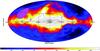 |
Fig. 1 Hammer-Aitoff projection of the 45 MHz full sky map. Eight contours are drawn between 15 000 and 60 000 K. The map does not cover the δ > +65° zone. |
Parameters of the Northern and Southern surveys.
An important characteristic of the all-sky 45 MHz map is that it consists of only two surveys and uses only two transit instruments with similar characteristics. Some relevant features of this map are:
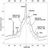 |
Fig. 2 Temperature averaged across latitude in the |b| < 10° strip from 45 MHz (continuous) and 408 MHz (dashed) surveys in arbitrarily normalized units: T(45 MHz)/(54 000 K) and T(408 MHz)/(300 K). The “steps” mark the tangential directions to spiral arms. |
-
1.
Galactic plane: most of the emission at 45 MHzcomes from the plane of the Galaxy that has an overall maxi-mum near the Galactic center. Figure 2 shows theplane profiles averaged inside the |b| < 10° strip for the 45 and 408[en-tity!#xa0!]MHz surveys, both convolved to the common 5° × 5°resolution. We can see that most of the structure of the 408[en-tity!#xa0!]MHz Galactic plane is reproduced in the 45[en-tity!#xa0!]MHz plane. This structure includes the strongmaximum near the Galactic center (note that the 45 MHz mapreaches its maximum at approximately l = 2°, as discussed in Alvarezet al. 1997a), the “steps” in theemission produced by the spiral arms can be seen tangentially,and some strong sources exist near the plane. The 45[en-tity!#xa0!]MHz map shows more conspicuously sourcesassociated with non-thermal emission (such as the Galacticcenter and Cas A), compared to the 408[en-tity!#xa0!]MHz map that shows strong thermal sources as well.
-
2.
Northern spur: this feature forms an arc from l ≈ 35°, b ≈ 16° passing through l ≈ 0°, b ≈ 75° and ending near the position of Virgo A.The hypothesis that this is a nearby supernova remnant shell is an old one (Hanbury Brown et al. 1960) and has become widely accepted (see Wolleben 2007, and references therein).
-
3.
Galactic and extragalactic sources: i) Galactic: SNR Cas A (l = 111.5° b = −2.3°), Vela SNR (l = 263.9° b = −3.3°), and the direction of the Local arm towards Cygnus and Vela. ii) Extragalactic: radio-galaxies such as Cen A (l = 309.5°, b = 19.4°), Cyg A (l = 76.2°, b = 5.8°), Virgo A (l = 285°, b = 74.3°), Hydra A (l = 243°, b = +25°), Pictor A (l = 252°, b = −34°), and Fornax A (l = 240°, b = −56.3°). We can also distinguish the Large Magellanic Cloud at l = 280.2°, b = −32.8°.
-
4.
Minimum temperature zones: there are two areas with minima of temperature, one in the southern Galaxy (l ~ 235°,b ~ −45°, T ~ 3600 K) and the other in the north (l ~ 192°,b ~ 48°, T ~ 3800 K). It is remarkable that these two points are rather close in Galactic longitude, at approximately the point where the Galactic plane reaches its minimum temperature compared to other longitudes (T ~ 8000 K, l ~ 225°, see Fig. 2). It is in these directions that any extragalactic or instrumental feature should be most noticeable. These two zones are later discussed in detail.
3. Spectral index map
From observations at two frequencies ν1 and
ν2, we can derive the “temperature spectral index”
βν1 − ν2
between these frequencies, defined as  (1)where
Tν1 and
Tν2 are the respective
brightness temperatures.
(1)where
Tν1 and
Tν2 are the respective
brightness temperatures.
At 45 and 408 MHz, the relation between the brightness temperature and the intensity of the radiation approximately follows the Rayleigh-Jeans law, which implies that it is a simple relation between the temperature spectral index β and the intensity spectral index α given by β = α + 2.
To calculate these spectral indices appropriately it is necessary to use brightness temperatures measured at the same resolution. Because of the difference in beam-size (and shape) between the surveys at 45 and 408 MHz, we convolved each map to 5°FWHM.
The measured temperature Tν at frequency
ν is modeled as  (2)with
a Galactic component Tν,G and an isotropic one
Tν,0 (the “offset”), which includes the
non-thermal extragalactic background (TEx), the
CMB (TCMB), and a zero-level correction
(TZLC). To obtain a spectral index associated with Galactic
emission, we need to correct the observed temperature by subtracting the offset temperature.
If the spectral index β due to Galactic emission is constant in some area,
then the following relations hold:
(2)with
a Galactic component Tν,G and an isotropic one
Tν,0 (the “offset”), which includes the
non-thermal extragalactic background (TEx), the
CMB (TCMB), and a zero-level correction
(TZLC). To obtain a spectral index associated with Galactic
emission, we need to correct the observed temperature by subtracting the offset temperature.
If the spectral index β due to Galactic emission is constant in some area,
then the following relations hold: 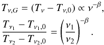 (3)
(3)
3.1. Zero-level correction of the 45 and 408 MHz surveys
On the basis of published data at different frequencies, we constructed a multi-frequency spectrum at selected and well-observed positions of the sky. We use these spectra to determine the zero-level correction temperature for the 45 and 408 MHz surveys.This zero level is a second order correction to the already calibrated data, and the method presented here is an alternative to the more common approach of using TT-plots (see e.g. Reich & Reich 1988a). The six selected positionsare:
-
The Galactic poles and the anticenter: these regions werechosen because we expect a minimal amount of Galactic thermalabsorption in these directions.
-
The directions of minimum temperature at 45 MHz in the northern (l = 192° , b = 48°) and southern (l = 235° , b = −45°) Galactic hemispheres: these directions were selected because the spectral index calculated in these zones is very sensitive to any correction applied to the data.
-
The “calibration point” (l = 38° , b = −1°): so-called because it was used to calibrate the 45 MHz southern survey (Alvarez et al. 1997b).
Multi-frequency spectral data corresponding to these six positions are given in Table 2. Whenever these values were not in digital format in the literature, they were read directly from the published contour maps. If the publication does not provide an estimate of the errors, we use plus-minus half of the difference between the closest contours.
Multifrequency data for the selected points.
We applied two extragalactic corrections TCMB and Tν,Ex (see Eq. (2)):
-
The 2.7 K of the CMB represents differentpercentages of the sky brightness temperature depending on theposition, but especially on the frequency ν of the radiation. While atfrequencies such as 45 MHz, where the minimumtemperature is close to 3500 K, this correction isnegligible, it is not at 408 MHz, where theminimum gets close to 13 K.
-
The extragalactic non-thermal background. This component is believed to originate from the integrated emission of non-resolved extragalactic radio sources. Appendix A gives arobust estimate of this extragalactic non-thermal spectrum (ENTS, Fig. A.1). We subtract this spectrum from every multifrequency plot, in addition to the 45 and 408 MHz data. This extragalactic emission corresponds to ~1100 K at 45 MHz and ~2.4 K at 408 MHz.
Figures 3 and 4 show the spectra of the six chosen zones together with least squares (in the log-log scale) fitted lines. Both extragalactic components have been subtracted from the data, and the defined multi-frequency spectral index is the slope of this line. In Table 2, the * symbol indicates that the point is not included in the least squares fitting. We neglected as an outlier one data value from the calibration point multifrequency fit (Fig. 4, bottom panel). This value, corresponding to 38 MHz (Blythe 1957), lies above the fit by a factor of ~3. We also neglected the data from the minimum south point below 45 MHz, for reasons we detailed below. Neglected data are marked by triangles in Figs. 3 and 4, where the 45 and 408 MHz data are identified by squares. Large discrepancies could be due to real physical features such as thermal absorption at very low frequencies, the steepening of the spectral index towards higher frequencies, instrumental calibration errors, etc. The points in the minimum-south plot (Fig. 3, bottom panel) below 45 MHz were also ignored because we believe they do not represent the real emission of this zone as the large beams associated with these surveys (from 7°to 15°FWHM) wash-out the relatively small area of the minimum-south. Figure 5 illustrates this effect: the contours delineate the minimum south, and the unresolved source just at the side seen in grey-scale is Fornax A, which also represents the 45 MHz antenna beam size. A larger beam would confuse the flux that surrounds the minimum zone (Fornax A flux inclusive) and would infer a higher temperature in this direction. This interpretation is confirmed in Fig. 3 where we can see that the fitted line to the data at frequencies above 45 MHz lies below of most of the data points measured at lower frequencies. We tested the spectra of the other five selected areas, and found that removing the low-frequency data does not affect the quality of the fittings significantly. In particular, the minimum-north zone is far more extended than the minimum-south zone, so the antenna beam size does not affect the measured temperature.
In Figs. 3 and 4, we did not include the points at 45 and 408 MHz in the fit because we are trying to find a correction applicable to these surveys based on independent data.
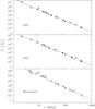 |
Fig. 3 Multi-frequency spectra of the Galactic component for (from top to bottom): south Galactic Pole, North Galactic Pole, and minimum-south zones. The triangles are not considered in the least squares fitting of the line. The squares represent the 45 and 408 MHz data. |
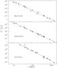 |
Fig. 4 Multi-frequency spectra of the Galactic component for the (from top to bottom) minimum-north, calibration point and anticenter zones. The triangles are not considered on the least squares fitting of the line. The squares represent the 45 and 408 MHz data. |
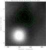 |
Fig. 5 Minimum-South zone, Plate-Careé projection and five equi-spaced contours between 3615 and 3870 K. No extragalactic correction applied. The source seen next to the contours is Fornax A. |
The coordinates of the six zones, the uncorrected temperatures at 45 and 408 MHz, and the
spectral index derived from these two values are given in Table 3. In contrast, Table 4 shows
temperature and spectral index values corrected by the extragalactic extended components,
that is, the ENTS and the CMB. The columns of Table 4 are: “extragalactic-corrected” temperatures, the “extragalactic-corrected”
spectral index derived between 45 and 408 MHz, the “extragalactic-corrected”
multifrequency spectral index, and the difference between these last two columns
( ).
).
We now explain the quantitative criterion used to evaluate the quality of the fits: having seen that extragalactic-corrected multi-frequency spectra are well fitted by single power laws, as expected if we observe non-thermal synchrotron radiation, we determine zero-level corrections (ZLC) to the 45 and 408 MHz maps such that, when applied uniformly to the six zones, they maximize the sum of the squares of the linear correlation coefficients of the six linear fits.
To summarize, reliable Galactic spectral indices between the 45 and 408 MHz can be derived by applying the ENTS, CMB and the ZLC corrections to both surveys. Table 5 displays all of these corrections. Table 6 shows the 45–408 MHz spectral index corrected values (corrected for ENTS, CMB, and ZLC) and the differences between these corrected temperatures and the multifrequency fit (Tfit). These spectral indices and the map derived represent our best estimates of the Galactic temperature spectral index between these two frequencies.
The isotropic corrections
(Tν,0 = TCMB + Tν,Ex + Tν,ZLC
in Eq. (2)) are
 (4)Figure 6 shows the final spectral index map.
There are several considerations to take into account concerning the multifrequency spectrum procedure:
-
The different resolutions of the data. When comparing differentsurveys, we really should adopt a common resolution, which wedo not here. However, apart from the systematic errors in the mea-sured temperatures at low frequencies in the minimum-southzone, as already explained, the multifrequency spectra showremarkable agreement between independent measures and nosignificant departure from a single power-law fit. Excluding theminimum-south zone, the zones selected correspond to rela-tively extended and uniform areas at the resolution of the studieswe used. Therefore, differences in beam sizes should not affectsignificantly the temperature measured in these directions.
-
Free-free absorption should produce departures from a single power law, specially at low frequencies that becomes significant at the “calibration point”, which is close to the Galactic plane towards the inner Galaxy. However, the spectrum shown in Fig. 4 (bottom panel) does not show any systematic departure from the straight line fit, at least one that is noticeable beyond the scatter of the points. Therefore, a single power-law seems to be a reasonable fit in each zone.
-
Apart from the intrinsic shortcomings of the multifrequency data caused by their low resolution, we believe that these data are very consistent and, in general, we did not find calibration or instrumental errors that question their quality. The determination of spectral indices by means of multifrequency power-law fits should be statistically stronger.
Uncorrected temperatures and spectral index.
Extragalactic corrected temperatures and spectral indices.
4. Discussion of the maps
4.1. Scanning and matching effects
The data from low-frequency Galactic surveys are usually obtained by scanning the sky with transit instruments. By “scanning effects”, we refer to the stripes produced in the temperature maps (and particularly noticeable in the spectral index map) because of the different observing conditions, e.g. differences in gain or ionospheric absorption, between adjacent scans made by the instrument. Another spurious effect is produced when surveys made at different epochs or zones or with different instruments are combined in a process described, for example, in Haslam et al. (1981) where the 408 MHz all-sky map was obtained. This effect is caused by the matching of partial maps that together form the final map, and we refer to this as the “matching effect”. All these spurious features and residues are usually produced along constant declination and/or right ascension.
The 45 MHz map has a matching effect produced by combining the northern and southern surveys at δ ≈ 10°. Maeda et al. (1999) calibrated the northern 45 MHz survey using data of the southern survey in a strip of the sky observed with both instruments. The same procedure was used to create the all-sky 45 MHz map presented in this paper. Scanning effects in this survey are present especially at the positions RA: 15 h ≲ RA ≲ 24 h and −30° ≲ Dec ≲ 30°. They appear at constant declination because both radio telescopes used in the 45 MHz survey were transit instruments. Stripes in the spectral index map at constant RA are due to scanning and matching effects associated with the 408 MHz map, which is formed by combining six different surveys as described in Haslam et al. (1981, Fig. 1). Both effects are more important near the zones where the temperature reaches a minimum and are far more noticeable in the spectral index map rather than in the temperature map. The effects described produce some systematic errors in our spectral index at a level lower than 0.05.
4.2. Principal physical processes and characteristics
The principal emission mechanism at 45 MHz is synchrotron radiation from relativistic
electrons that permeates the interstellar medium (ISM). The emissivity at a frequency
ν is proportional to  ,
where (−ϵ) is the exponent of an assumed power-law distribution of the
relativistic electrons energy and H is the magnitude of the magnetic field. A study of
synchrotron emission alone cannot differentiate between the effect of the magnetic field
and the characteristics of the fast electron population. Using pulsar rotation measures,
Han et al. (2006) placed constraints on the
global magnetic field (2 ~ 3 μG on average in the ISM). Testori et al. (2008) also note from polarization maps
of the 21 cm continuum that the polarized radio emission is only a few percent (5%) of the
total radiation. This may imply that on Galactic scales the “random” component of the
magnetic field is far more important than coherent field zones. If this were the case,
synchrotron emission would give a direct way of obtaining the relativistic electron column
density. If, however, as the three-dimensional Galactic models of Sun et al. (2008) suggest, the regular field is comparable and even
more intense than the random field, then the relativistic electron column density can only
be obtained from the synchrotron emission with the knowledge of the direction of the
regular magnetic field.
,
where (−ϵ) is the exponent of an assumed power-law distribution of the
relativistic electrons energy and H is the magnitude of the magnetic field. A study of
synchrotron emission alone cannot differentiate between the effect of the magnetic field
and the characteristics of the fast electron population. Using pulsar rotation measures,
Han et al. (2006) placed constraints on the
global magnetic field (2 ~ 3 μG on average in the ISM). Testori et al. (2008) also note from polarization maps
of the 21 cm continuum that the polarized radio emission is only a few percent (5%) of the
total radiation. This may imply that on Galactic scales the “random” component of the
magnetic field is far more important than coherent field zones. If this were the case,
synchrotron emission would give a direct way of obtaining the relativistic electron column
density. If, however, as the three-dimensional Galactic models of Sun et al. (2008) suggest, the regular field is comparable and even
more intense than the random field, then the relativistic electron column density can only
be obtained from the synchrotron emission with the knowledge of the direction of the
regular magnetic field.
The principal absorption mechanism at 45 MHz is thermal absorption from warm (~8000 K) ionized hydrogen. This absorption diminishes the spectral index in the Galactic plane with respect to that at higher latitude. In the multifrequency data, we have seen no obvious absorption feature or departures from a straight-line fit not even in the calibration-point zone (spectral index 2.28), where it would be expected because it is closer to the Galactic plane and in the direction of the inner Galaxy. An absorbed spectra may not differ very much from a non-absorbed one across this range of frequencies. Figure 7 presents two fits to the calibration-point data assuming that the absorption occurs homogeneously along the line of sight. The one displayed with a continuous line assumes that the non-absorbed, purely emission spectrum has an spectral index of 2.48 (the anticenter value), while the other (dashed line), uses a steeper spectrum with spectral index of 2.8. The values derived for EM/(cm-6pc) × (Te/1000 K)-1.35, where EM is the emission measure and Te is the electron temperature, are 482 and 455, very close to the 470 obtained by Jones & Finlay (1974) towards the l = −35°,b = 0° direction, which is located in an approximately symmetrical longitude about the Galactic center with respect to the calibration-point (l = 38°,b = 1°). Both fittings are fairly reasonable, and the absorption column can take account of the flattening of the spectrum. The emission measures derived assuming 5000 K < Te < 8000 K for the warm ionized gas to produce the absorption seen in the spectral index map are between 1600 and 4000 pc cm-6, well above the emission measures from the warm ionized medium (Hill et al. 2008). We conclude that this absorption is produced mainly in HII-regions, unresolved by the present survey, implying that the emission measures derived should be regarded as beam-averaged values.
Temperature offset corrections in K.
Corrected 45–408 MHz spectral indices and differences between the corrected temperatures and the multifrequency fit.
An important characteristic of the map is the presence of two minimum temperature zones, whose multifrequency spectra are shown in Figs. 3 and 4, in the bottom and top panels, respectively. They do not exhibit absorption in the spectral index map discernible by means of a flatter spectrum or a turn-over towards lower frequencies in the multifrequency data. The two zones could be a single volume with either a low density of relativistic electrons or weak magnetic fields. This volume should be nearby judging from its large extension in the sky. There appears to be little correlation with the local bubble described in Lallement et al. (2003), but the positions of the minima are consistent with the super bubble found by Heiles (1998). Interpreting the minimum zones as being produced by a bubble is consistent with both the little absorption detected in their directions and the interpretation of Sun et al. (2008) that high-latitude radio emission comes not from an extended halo-zone but primarily from a local excess of synchrotron emissivity: a local bubble could then explain the minima in these directions. The polarization map of Testori et al. (2008) does not show any conspicuous enhancement or decrement in the polarization fraction toward the southern minimum. We also note that the temperatures measured towards the minima can be considered as upper limits to the extragalactic background.
The maximum spectral index (~2.7) is found in a rather flat plateau of approximately 15°diameter around l ~ 70°, b ~ +25° adjacent to the Northern Spur. This feature is consistent with the results obtained by Webster (1974) (at δ = 40°) and Lawson et al. (1987) who found a steepening of the spectrum in this zone, that is, on the ridge of the Northern Spur rather than on the spur itself. This area of high spectral index is also noted by Roger et al. (1999) between 22 and 408 MHz.
The mean values of the spectral index are consistent with studies made at similar frequencies, for example, Purton (1966) found an spectral index in the halo-high latitude zone of 2.57, close to our mean of 2.54 and Sironi (1974) found a spectral index of 2.53 in the minimum-north between 81.5 and 408 MHz (our value is 2.47). Agreement is better if the zones compared have a relatively constant spectral index because in this case the difference in beam sizes does not affect the spectral index. In contrast, when looking at the anticenter, Purton gets 2.55, a higher value than ours, but within our errors.
The all-sky map compiled by Reich & Reich (1988a) measures spectral indices that are systematically higher by about 0.2 than our map. Webster (1974), who measured the spectral index between 408 and 610 MHz, also obtained values slightly larger than ours. In general, the spectral index appears to increase slightly with frequency in every zone, probably because of aging of the relativistic electron population. The increase in spectral index with frequency on Galactic scales is also obtained by de Oliveira-Costa et al. (2008) through their negative γ-parameter at least at ν ≲ 1 GHz, where synchrotron dominates over free-free or the CMB. We do not see a flattening of the spectrum with increasing Galactic latitude at l ~ 180° as described in Reich & Reich (1988b).
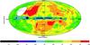 |
Fig. 6 Galactic temperature spectral index between 45 and 408 MHz with the corrections of Table 6 applied. The map has 5° × 5° resolution. |
5. Conclusions
We have presented a 45 MHz survey that covers more than 95% of the sky and has the advantage of being assembled by data taken with only two radio telescopes of similar characteristics. This map shows the emission from the relativistic electrons being decelerated by the magnetic fields in the interstellar medium. There are two zones of minimum temperature toward l ~ 230° that are located more or less symmetrically with respect to the Galactic plane. They presumably belong to a single local decrement in the density of relativistic electrons or of the magnetic field magnitude.
We have used this map together with the 408 MHz all-sky survey from Haslam et al. (1981) to produce an all-sky spectral index map. We have used a large literature compilation of data to: i) estimate the extragalactic non-thermal emission contribution; and ii) implement a method for finding zero-level corrections for radio surveys based on independent data.
The spectral index map has allowed us to derive some conclusions about overall Galactic features: the sky has spectral indices that range between 2.1 and 2.7. Over most of the sky, the index is between 2.5 and 2.6, which is reduced by thermal absorption to values between 2.1 to 2.5 across the Galactic plane strip (|b| < 10°). This absorption is probably due to HII regions rather than a more extended global structure such as the WIM. There is a large zone around l ~ 70°, b ~ +25° adjacent to the Northern Polar Spur where the average spectral index is close to the maximum of 2.7.
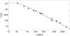 |
Fig. 7 Fittings to the calibration-point data using a thermally absorbed power-law spectrum with spectral index equal to that at the anticenter (2.48, continuous line) and the value used by Jones & Finlay (1974) (2.80, dashed). Both fittings are reasonable considering the dispersion in the data. |
We have also reviewed (Appendix A) estimates of the extragalactic non-thermal contribution in the low frequency range.
The 45 MHz map can be downloaded from the website http://www.das.uchile.cl/survey45mhz.
Acknowledgments
We would like to thank Dr. Patricia Reich for producing the 5° degraded resolution maps at 45 and 408 MHz. We would like to add a note in memory of our colleague Fernando Olmos (1958-2010) who actively collaborated in the construction and operation of the Maipu array, as well as in the analysis of its data. J.M. acknowledges partial support from Centro de Astrofísica FONDAP 15010003 and from Center of Excellence in Astrophysics and Associated Technologies (PFB 06).
References
- Allen, C. W., & Gum, C. S. 1950, Austral. J. Sci. Res. A Phys. Sci., 3, 224 [Google Scholar]
- Alvarez, H., Aparici, J., May, J., & Olmos, F. 1994, Exp. Astron., 5, 315 [NASA ADS] [CrossRef] [Google Scholar]
- Alvarez, H., Aparici, J., & May, J. 1997a, A&A, 327, 569 [NASA ADS] [Google Scholar]
- Alvarez, H., Aparici, J., May, J., & Olmos, F. 1997b, A&AS, 124, 315 [NASA ADS] [CrossRef] [EDP Sciences] [Google Scholar]
- Andrew, B. H. 1966, MNRAS, 132, 79 [NASA ADS] [Google Scholar]
- Andrews, B. H. 1969, MNRAS, 143, 17 [NASA ADS] [Google Scholar]
- Ariskin, V. I. 1981, Sov. Astron., 25, 558 [NASA ADS] [Google Scholar]
- Baldwin, J. E. 1955, MNRAS, 115, 684 [NASA ADS] [Google Scholar]
- Baldwin, J. E. 1967, in Radio Astronomy and the Galactic System, ed. H. van Woerden, IAU Symp., 31, 337 [Google Scholar]
- Berkhuijsen, E. M. 1972, A&AS, 5, 263 [NASA ADS] [Google Scholar]
- Blythe, J. H. 1957, MNRAS, 117, 652 [NASA ADS] [Google Scholar]
- Bolton, J. G., & Westfold, K. C. 1950, Austral. J. Sci. Res. A Phys. Sci., 3, 19 [NASA ADS] [Google Scholar]
- Bridle, A. H. 1967, MNRAS, 136, 219 [NASA ADS] [Google Scholar]
- Cane, H. V. 1979, MNRAS, 189, 465 [NASA ADS] [Google Scholar]
- Caswell, J. L. 1976, MNRAS, 177, 601 [NASA ADS] [Google Scholar]
- Clark, T. A., Brown, L. W., & Alexander, J. K. 1970, Nature, 228, 847 [NASA ADS] [CrossRef] [PubMed] [Google Scholar]
- de Oliveira-Costa, A., Tegmark, M., Gaensler, B. M., et al. 2008, MNRAS, 388, 247 [NASA ADS] [CrossRef] [Google Scholar]
- Dröge, F., & Priester, W. 1956, Z. Astrophys., 40, 236 [Google Scholar]
- Dwarakanath, K. S., & Udaya Shankar, N. 1990, J. Astrophys. Astron., 11, 323 [Google Scholar]
- Ellis, G. R. A. 1982, Austral. J. Phys., 35, 91 [Google Scholar]
- Ellis, G. R. A., & Hamilton, P. A. 1966, ApJ, 143, 227 [NASA ADS] [CrossRef] [Google Scholar]
- Ellis, G. R. A., & Mendillo, M. 1987, Austral. J. Phys., 40, 705 [NASA ADS] [Google Scholar]
- Fukao, S., Sato, T., Tsuda, T., Kato, S., & Wakasugi, K. 1985a, Radio Science, 20, 1155 [NASA ADS] [CrossRef] [Google Scholar]
- Fukao, S., Tsuda, T., Sato, T., et al. 1985b, Radio Science, 20, 1169 [NASA ADS] [CrossRef] [Google Scholar]
- Gervasi, M., Tartari, A., Zannoni, M., Boella, G., & Sironi, G. 2008, ApJ, 682, 223 [NASA ADS] [CrossRef] [Google Scholar]
- Hamilton, P. A., & Haynes, R. F. 1968, Austral. J. Phys., 21, 895 [NASA ADS] [Google Scholar]
- Hamilton, P. A., & Haynes, R. F. 1969, Austral. J. Phys., 22, 839 [NASA ADS] [Google Scholar]
- Han, J. L., Manchester, R. N., Lyne, A. G., Qiao, G. J., & van Straten, W. 2006, ApJ, 642, 868 [NASA ADS] [CrossRef] [Google Scholar]
- Hanbury Brown, R., Davies, R. D., & Hazard, C. 1960, The Observatory, 80, 191 [NASA ADS] [Google Scholar]
- Hartz, T. R. 1964, Nature, 203, 173 [NASA ADS] [CrossRef] [Google Scholar]
- Haslam, C. G. T., Quigley, M. J. S., & Salter, C. J. 1970, MNRAS, 147, 405 [NASA ADS] [Google Scholar]
- Haslam, C. G. T., Klein, U., Salter, C. J., et al. 1981, A&A, 100, 209 [NASA ADS] [Google Scholar]
- Haslam, C. G. T., Salter, C. J., Stoffel, H., & Wilson, W. E. 1982, A&AS, 47, 1 [NASA ADS] [Google Scholar]
- Heiles, C. 1998, ApJ, 498, 689 [NASA ADS] [CrossRef] [Google Scholar]
- Hill, E. R., Slee, O. B., & Mills, B. Y. 1958, Austral. J. Phys., 11, 530 [Google Scholar]
- Hill, A. S., Benjamin, R. A., Kowal, G., et al. 2008, ApJ, 686, 363 [NASA ADS] [CrossRef] [Google Scholar]
- Hornby, J. M., & Williams, P. F. S. 1966, MNRAS, 131, 237 [NASA ADS] [CrossRef] [Google Scholar]
- Howell, T. F. 1970, Astrophys. Lett., 6, 45 [NASA ADS] [Google Scholar]
- Jones, B. B., & Finlay, E. A. 1974, Austral. J. Phys., 27, 687 [Google Scholar]
- Ko, H. C., & Kraus, J. D. 1957, S&T, 16, 160 [NASA ADS] [Google Scholar]
- Lallement, R., Welsh, B. Y., Vergely, J. L., Crifo, F., & Sfeir, D. 2003, A&A, 411, 447 [EDP Sciences] [Google Scholar]
- Landecker, T. L., & Wielebinski, R. 1970, Austral. J. Phys. Astrophys. Suppl., 16, 1 [Google Scholar]
- Large, M. I., Mathewson, D. S., & Haslam, C. G. T. 1961, MNRAS, 123, 123 [NASA ADS] [Google Scholar]
- Lawson, K. D., Mayer, C. J., Osborne, J. L., & Parkinson, M. L. 1987, MNRAS, 225, 307 [NASA ADS] [CrossRef] [Google Scholar]
- Maeda, K., Alvarez, H., Aparici, J., May, J., & Reich, P. 1999, A&AS, 140, 145 [NASA ADS] [CrossRef] [EDP Sciences] [Google Scholar]
- Mathewson, D. S., Broten, N. W., & Cole, D. J. 1965, Austral. J. Phys., 18, 665 [Google Scholar]
- May, J., Reyes, F., Aparici, J., et al. 1984, A&A, 140, 377 [NASA ADS] [Google Scholar]
- Milogradov-Turin, J., & Smith, F. G. 1973, MNRAS, 161, 269 [NASA ADS] [Google Scholar]
- Moran, M. 1965, MNRAS, 129, 447 [NASA ADS] [Google Scholar]
- Pauliny-Toth, I. K., & Shakeshaft, J. R. 1962, MNRAS, 124, 61 [NASA ADS] [Google Scholar]
- Piddington, J. H. 1951, MNRAS, 111, 45 [NASA ADS] [Google Scholar]
- Piddington, J. H., & Trent, G. H. 1956, Austral. J. Phys., 9, 481 [Google Scholar]
- Price, R. M. 1972, AJ, 77, 845 [NASA ADS] [CrossRef] [Google Scholar]
- Purton, C. R. 1966, MNRAS, 133, 463 [NASA ADS] [Google Scholar]
- Reich, W. 1982, A&AS, 48, 219 [Google Scholar]
- Reich, P., & Reich, W. 1986, A&AS, 63, 205 [NASA ADS] [Google Scholar]
- Reich, P., & Reich, W. 1988a, A&AS, 74, 7 [Google Scholar]
- Reich, P., & Reich, W. 1988b, A&A, 196, 211 [NASA ADS] [Google Scholar]
- Reich, P., Testori, J. C., & Reich, W. 2001, A&A, 376, 861 [NASA ADS] [CrossRef] [EDP Sciences] [Google Scholar]
- Reich, P., Reich, W., & Testori, J. C. 2004, in The Magnetized Interstellar Medium, ed. B. Uyaniker, W. Reich, & R. Wielebinski, 63 [Google Scholar]
- Roger, R. S., Costain, C. H., Landecker, T. L., & Swerdlyk, C. M. 1999, A&AS, 137, 7 [NASA ADS] [CrossRef] [EDP Sciences] [Google Scholar]
- Rohan, P., & Soden, L. B. 1970, Austral. J. Phys., 23, 223 [NASA ADS] [Google Scholar]
- Seeger, C. L., Westerhout, G., Conway, R. G., & Hoekema, T. 1965, Bull. Astron. Inst. Netherlands, 18, 11 [NASA ADS] [Google Scholar]
- Shain, C. A. 1951, Austral. J. Sci. Res. A Phys. Sci., 4, 258 [NASA ADS] [Google Scholar]
- Shain, C. A. 1959, in URSI Symp. 1: Paris Symposium on Radio Astronomy, ed. R. N. Bracewell, IAU Symp., 9, 328 [Google Scholar]
- Shain, C. A., & Higgins, C. S. 1954, Austral. J. Phys., 7, 130 [Google Scholar]
- Simon, A. J. B. 1977, MNRAS, 180, 429 [NASA ADS] [Google Scholar]
- Sironi, G. 1974, MNRAS, 166, 345 [NASA ADS] [Google Scholar]
- Sun, X. H., Reich, W., Waelkens, A., & Enßlin, T. A. 2008, A&A, 477, 573 [NASA ADS] [CrossRef] [EDP Sciences] [Google Scholar]
- Testori, J. C., Reich, P., & Reich, W. 2008, A&A, 484, 733 [NASA ADS] [CrossRef] [EDP Sciences] [Google Scholar]
- Turtle, A. J., & Baldwin, J. E. 1962, MNRAS, 124, 459 [NASA ADS] [CrossRef] [Google Scholar]
- Véron, P. 1967, Annales d’Astrophysique, 30, 719 [NASA ADS] [Google Scholar]
- Wall, J. V., Chu, T. Y., & Yen, J. L. 1970, Austral. J. Phys., 23, 45 [Google Scholar]
- Webster, A. S. 1974, MNRAS, 166, 355 [NASA ADS] [CrossRef] [Google Scholar]
- Wielebinski, R., Smith, D. H., & Garzón Cárdenas, X. 1968, Austral. J. Phys., 21, 185 [NASA ADS] [Google Scholar]
- Wolleben, M. 2007, ApJ, 664, 349 [NASA ADS] [CrossRef] [Google Scholar]
- Yates, K. W. 1968, Austral. J. Phys., 21, 167 [Google Scholar]
- Yates, K. W., & Wielebinski, R. 1965, Nature, 208, 64 [NASA ADS] [CrossRef] [Google Scholar]
- Yates, K. W., Wielebinski, R., & Landecker, T. L. 1967, Austral. J. Phys., 20, 595 [Google Scholar]
Appendix A: The extragalactic background spectrum
The knowledge of the extragalactic non-thermal spectrum (ENTS), besides its importance on its own, permits a more accurate determination of the emission of our own Galaxy and is another “foreground” component for CMB studies. To separate the radio emission of our own Galaxy from this extragalactic background emission, we have searched the literature to find a reliable estimate of the ENTS. Table A.1 displays the works selected for their original estimate of the extragalactic background component. We note that although this is considered an important issue in most radio surveys, only a few authors have made attempts to estimate it:
Extragalactic data obtained from the literature.
-
i)
The most common approach is to consider the ENTSas the integrated contribution of extragalactic radiosources, extrapolating their population and distribu-tion from catalogs, and using a cosmological model.Bridle (1967); Simon (1977); Lawsonet al. (1987), and Gervasiet al. (2008) used and described themethod in detail. In general, the ENTS derived has a spectral indexthat is about 0.1−0.2 higher than the average emission from our own Galaxy or any other “normal” galaxy. This is attributed probably to the influence of the scarcer but much more luminous radio-galaxieson the ENTS.
-
ii)
Another less common approach is to model the Galactic emission to extract it from the measured data. Yates (1968) and Cane (1979) used simple models consisting of axisymmetric cylindrical components plus arms, spurs, and Galactic sources.
-
iii)
Shain (1959) used 30-Doradus as a thermal absorption screen that at low frequencies blocks the ENTS. Comparison of the emission measured along its line of sight with a nearby one, not-blocked by this HII-region, would cancel out the Galactic component and leave the extragalactic emission.
-
iv)
Baldwin (1967) uses differential spectra to cancel the ENTS and obtain tighter constraints on the Galactic spectrum, which, together with an adequate treatment of the instrumental components, would permit us to obtain the ENTS.
Figure A.1 shows a single power-law fit to the
temperatures shown in Table A.1. The best-fit
solution is given by  (A.1)Whenever the publication
was not explicit about the uncertainty in the derived value, we assume it to be twice as
large as the errors in the data from where the extragalactic component was derived. From
the uncertainty in the data points, we estimate the error in the derived ENTS spectral
index to be ≳0.04.
(A.1)Whenever the publication
was not explicit about the uncertainty in the derived value, we assume it to be twice as
large as the errors in the data from where the extragalactic component was derived. From
the uncertainty in the data points, we estimate the error in the derived ENTS spectral
index to be ≳0.04.
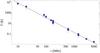 |
Fig. A.1 Extragalactic component estimates and a single power-law fit. |
All Tables
Corrected 45–408 MHz spectral indices and differences between the corrected temperatures and the multifrequency fit.
All Figures
|
Fig. 1 Hammer-Aitoff projection of the 45 MHz full sky map. Eight contours are drawn between 15 000 and 60 000 K. The map does not cover the δ > +65° zone. |
| In the text | |
|
Fig. 2 Temperature averaged across latitude in the |b| < 10° strip from 45 MHz (continuous) and 408 MHz (dashed) surveys in arbitrarily normalized units: T(45 MHz)/(54 000 K) and T(408 MHz)/(300 K). The “steps” mark the tangential directions to spiral arms. |
| In the text | |
|
Fig. 3 Multi-frequency spectra of the Galactic component for (from top to bottom): south Galactic Pole, North Galactic Pole, and minimum-south zones. The triangles are not considered in the least squares fitting of the line. The squares represent the 45 and 408 MHz data. |
| In the text | |
|
Fig. 4 Multi-frequency spectra of the Galactic component for the (from top to bottom) minimum-north, calibration point and anticenter zones. The triangles are not considered on the least squares fitting of the line. The squares represent the 45 and 408 MHz data. |
| In the text | |
|
Fig. 5 Minimum-South zone, Plate-Careé projection and five equi-spaced contours between 3615 and 3870 K. No extragalactic correction applied. The source seen next to the contours is Fornax A. |
| In the text | |
|
Fig. 6 Galactic temperature spectral index between 45 and 408 MHz with the corrections of Table 6 applied. The map has 5° × 5° resolution. |
| In the text | |
|
Fig. 7 Fittings to the calibration-point data using a thermally absorbed power-law spectrum with spectral index equal to that at the anticenter (2.48, continuous line) and the value used by Jones & Finlay (1974) (2.80, dashed). Both fittings are reasonable considering the dispersion in the data. |
| In the text | |
|
Fig. A.1 Extragalactic component estimates and a single power-law fit. |
| In the text | |
Current usage metrics show cumulative count of Article Views (full-text article views including HTML views, PDF and ePub downloads, according to the available data) and Abstracts Views on Vision4Press platform.
Data correspond to usage on the plateform after 2015. The current usage metrics is available 48-96 hours after online publication and is updated daily on week days.
Initial download of the metrics may take a while.