| Issue |
A&A
Volume 523, November-December 2010
|
|
|---|---|---|
| Article Number | A65 | |
| Number of page(s) | 7 | |
| Section | Stellar atmospheres | |
| DOI | https://doi.org/10.1051/0004-6361/201015361 | |
| Published online | 18 November 2010 | |
Abundances in the Herbig Ae star HD 101412
Abundance anomalies; λ Boo–Vega characteristics?⋆
1
Department of Astronomy, University of Michigan,
Ann Arbor,
MI
48109-1090,
USA
e-mail: This email address is being protected from spambots. You need JavaScript enabled to view it.
2
AIP, An der Sternwarte 16, 14482
Potsdam,
Germany
e-mail: This email address is being protected from spambots. You need JavaScript enabled to view it.
3
Instituto de Ciencias Astronómicas, del la Terra y del Espacio, Casilla 467,
5400
San Juan,
Argentina
e-mail: This email address is being protected from spambots. You need JavaScript enabled to view it.
4
Institute of Astronomy, Russian Academy of Sciences,
Pyatnitskaya 48,
Moscow
119017,
Russia
e-mail: This email address is being protected from spambots. You need JavaScript enabled to view it.
Received:
7
July
2010
Accepted:
9
August
2010
Abstract
Context. Recent attention has been directed to abundance variations among very young stars.
Aims. We perform a detailed abundance study of the Herbig Ae star HD 101412, taking advantage of its unusually sharp spectral lines.
Methods. High-resolution spectra are measured for accurate wavelengths and equivalent widths. Balmer-line fits and ionization equlibria give a relation between Teff, and log (g). Abundance anomalies and uncertain reddening preclude the use of spectral type or photometry to fix Teff. Excitation temperatures are used to break the degeneracy between Teff and log (g).
Results. Strong lines are subject to an anomalous saturation that cannot be removed by assuming a low microturbulence. By restricting the analysis to weak (≤20 mÅ) lines, we find consistent results for neutral and ionized species, based on a model with Teff = 8300 K, and log (g) = 3.8. The photosphere is depleted in the most refractory elements, while volatiles are normal or, in the case of nitrogen, overabundant with respect to the sun. The anomalies are unlike those of Ap or Am stars.
Conclusions. We suggest the anomalous saturation of strong lines arises from heating of the upper atmospheric layers by infalling material from a disk. The overall abundance pattern may be related to those found for the λ Boo stars, though the depletions of the refractory elements are milder, more like those of Vega. However, the intermediate volatile zinc is depleted, precluding a straightforward interpretation of the abundance pattern in terms of gas-grain separation.
Key words: stars: chemically peculiar / stars: abundances / stars: individual: HD 101412 / stars: pre-main sequence / stars: early-type
Based on observations obtained at the European Southern Observatory, Paranal and La Silla, Chile (ESO programmes 077.C-0521(A), 081.C-0410(A) and 383.C-0684(A).
© ESO, 2010
1. Introduction
The star HD 101412 (CD −59 3865, V1052 Cen) belongs to the group of Herbig Ae/Be stars, whose members are considered more massive counterparts of T Tauri pre-main sequence stars. Masses range from 2−10 M⊙ (Hernández et al. 2005). Their spectral energy distribution is characterized by the presence of an infrared excess due to thermal re-emission of circumstellar dust, which is thought to be the signature of a circumstellar disk (cf. Hartmann 2009, Sect. 8.8). According to Fedele et al. (2008) HD 101412 is a group II source (using the classification of Meeus et al. 2001), with the flat disk self-shadowed by dust. Wade et al. (2005) discussed HD 101412 as a possible progenitor of magnetic chemically peculiar (CP2 or Ap) stars. A number of recent studies have been devoted to this star (cf. Hubrig et al. 2009, 2010), including an estimate of its metallicity (Guimarães et al. 2006). The absorption lines are unusually sharp, leading to suggestions that the star may be seen nearly “pole on”. Intrinsically slow rotation cannot be excluded. Indeed, Fedele et al. (2008) propose a model with a disk inclined by 20° to the line of sight, a model now supported by a newly-found photometric period.
Very recent work shows that HD 101412 is a low-amplitude photometric variable with the period of 42ḍ0 (Mikulášek et al., in prep.). If the period is a rotational one, it then comports well with our spectroscopic value, v·sini = 3 ± 1 km s-1, and excludes a conclusion that the narrow lines could only be due to a (nearly) pole-on viewing angle.
Numerous emission features in Herbig Ae stars indicate an atmospheric structure that must differ from the classical, one-dimensional models typically used for abundance analyses. Nevertheless, abundance work on these objects has been attempted (cf. Guimarães et al. 2006; Acke & Welkens 2004). The latter study is of particular interest to the results presented here, as the authors sought the signature of the λ Boo phenomena, citing the seminal paper by Venn & Lambert (1990). These authors noted that the most volatile elements, C, N, and O showed mild abundance depletions, while the more refractory elements showed significant depletions, 1 dex or more. They noted the similarity of these depletions to those of the interstellar gas which is well correlated with condensation temperatures (cf. Sect. 7).
The sharp spectral lines of HD 101412 make it ideal for abundance work. Although a magnetic field has been detected (cf. Wade et al. 2005), magnetic enhancement of the lines is masked by other factors, to be discussed below (Sect. 5). Hubrig et al. (2010) noted that the Zeeman patterns of several lines were resolved, or partially resolved. Nevertheless, most atomic lines are sufficiently sharp that numerous relatively unblended lines could be found for abundance work.
2. Spectra
The current paper is based on a subset of the spectra described by Hubrig et al. (2010). Most equivalent widths were measured on two HARPS spectra (averaged) obtained in 2009 on 23:47 UT of 4 July, and 00:13 UT of 5 July. About 10 per cent of the equivalent widths are from UVES spectra obtained on 9 (visual and IR) and 15 April (UV) 2009.
Wavelengths were measured on the HARPS spectrum in the range λλ3782−6911. The averaged spectra were subjected to mild Fourier filtering. Signal-to-noise estimates, made directly from the filtered spectra average 148. HARPS spectra have a resolving power (RP) of 120 000, but averaging and filtering reduce this to an estimated 40 000. Fortunately, equivalent widths are independent of RP; we exchange RP for noise reduction.
We have used accurate wavelength measurements both for line identification, and to find relatively unblended lines.
The UVES spectrum obtained on 15 April 2009, was measured for wavelengths in the range λλ3301−4517. A few equivalent widths below the Balmer Limit were obtained from this spectrum.
Additional wavelengths were measured from UVES spectra taken on 9 April 1999 (λλ6911−7519 and 7661−9461). The Ca ii infrared triplet was examined for possible isotopic shifts discovered by Castelli & Hubrig (2004). The lines were shifted by 0.02 to 0.03 Å with respect to the solar wavelengths of these lines, a rather small shift that could be entirely due to measurement error.
Hubrig et al. (2010) demonstrate equivalent width changes of the order of 20% (0.08 dex). The variations were correlated with an assumed phase, 1386 days nearly one third the newly determined period of 420. Also possible, are line strength changes due to time-dependent motions of the circumstellar material. These variations must be kept in mind in evaluating the abundances which were determined here primarily from a single phase. An error of 0.08 dex is marginally significant, relative to other uncertainties in the abundances (cf. Table 2).
Balmer line profiles were measured on a FORS 1 spectrum obtained on 22 May 2008, in visitor mode at ESO. We used the (200 kHz, low, 1 × 1) readout mode, which makes it possible to achieve a S/N ratio of about 1000−1200 with a single exposure and the GRISM 600B in the wavelength range 3250−6215 Å to cover all hydrogen Balmer lines from Hβ to the Balmer jump. A slit width of 0 4 was used to obtain a spectral resolving power of R ≈ 2000. Details of data reduction are given by Hubrig et al. (2004).
3. Model atmospheres and spectral calculations
All model atmospheres are based on T − τ relations from the version of ATLAS9 (Kurucz 1993) of the Trieste group (cf. Sbordone et al. 2004). Given T(τ), the depth integrations from log (τ5000) of −5.4 to + 1.4 were carried out with software and opacity routines written and used at Michigan for several decades. Agreement with ATLAS9 Models posted on Castelli’s (2010) site are excellent (see Castelli & Kurucz 2003). Spot checks using WIDTH9 for weak Fe i and ii lines, which are independent of the different damping constants of the two codes, show agreement within 0.02 dex. Weak lines have equivalent widths of 20 mÅ or less.
4. Fixing the atmospheric parameters
4.1. Colors and spectral type
Broad and intermediate-band photometric measurements are typically used to fix the effective temperatures prior to an abundance analysis. Johnson (Vieira et al. 2003) and Geneva (Mermillod et al. 2007) indices are available for HD 101412; we found no Strömgren photometry. Unfortunately, the reddening correction is most uncertain. For example, Vieira et al.’s U − B = 0.15, B − V = 0.18 do not lead to an intersection with a standard U − B vs. B − V plot for either main sequence stars (Cox 2000, Table 15.7) or a ZAMS (Table 15.9). Since the star is known to be peculiar and variable, currently available photometry is not adequate to fix the effective temperature.
The spectral type of HD 101412 is given variously as B9-A0 V-III (e.g. B9/A0 V, Houk & Cowley 1975). According to Cox (2000), luminosity class V stars have effective temperatures in the range 10 500 to 9790 K, while we conclude Teff ≈ 8300 K. The spectral type of normal stars of this class depend strongly on the Ca ii K-line, or rather its strength relative to Ca ii H+Hϵ. The intensity of the Ca ii lines would be significantly diminished by the ≈ 0.6 dex underabundance we find for this element.
We conclude that the spectral type is not a useful indicator of the temperature of the star, or of the total absorption, AV.
4.2. The Balmer lines
Balmer line profiles are difficult to work with on high-dispersion material. This is especially true for echelle spectra, as the broad lines typically span echelle orders. We have attempted to fit profiles from an averaged HARPS spectrum, but have relied primarily on the FORS1 spectrum (Sect. 2) which included Hβ and higher members of the Balmer series (Fig. 1).
Guimarães et al. (2006) made use of Balmer lines but did not discuss Teff − log (g) degeneracy. They conclude Teff = 10000 ± 1000 K (see their Table 2). In Hubrig et al. (2009), only the wings of Hβ were used to find the atmospheric parameters, Teff = 10000, log (g) = 4.2−4.3. The authors note that a 9000 K, log (g) = 4.0 model also gave a good fit to the Hβ profile, but that with these parameters “many narrow lines” were seen in the synthetic spectrum that did not appear in the observed spectrum. These lines might not have appeared in the calculated spectrum if the abundances were low, as we currently assume.
The Hubrig et al. (2009) results show that within the relevant temperature range for HD 101412, the Balmer profiles are sensitive to both temperature and gravity. Our current calculations show that quite good fits to the Balmer profiles may be obtained for a temperature as low as 8300 K, if a log (g) = 3.8 is assumed (see Fig. 1). A still lower temperature could be accommodated by assuming an even lower gravity.
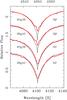 |
Fig. 1 Hβ (above, top wavelength scale) and Hδ profiles (bottom wavelength scale) for Teff = 8300 K, log (g) = 3.8 and 9800 K, log (g) = 3.8. Observed profiles are in gray (red in online version) with dots. The fits for the lower temperature are as good or arguably better than at the higher temperature. The relative flux scale is correct for the lowest profile pair. Upper pairs are successively raised by 0.4 units. |
Wavelength measurements of the cores of the Balmer lines on the FORS1 spectra show systematic red shifts that increase systematically from about +9 at H19 to +23 km s-1 at Hβ. Core shifts are marginally detectable in Fig. 1
4.3. Ionization equilibrium
We assume here that an optimum model will yield the same abundances from two stages of ionization of a given element. In a preliminary approach to obtain model parameters, we adopted a grid of temperatures and gravities shown in Table 1. The grid was chosen to bracket the expected stellar parameters. Provisional abundances were then calculated from equivalent width measurements of Fe i and ii lines using models with the parameters given in the table.
Provisional abundances (log (Fe / Ntot)) from Fe i and Fe ii for various temperatures and surface gravities.
A relation between Teff and log (g) is obtained as follows. For each of the three values of log (g), we plot log (Fe / Ntot) vs. Teff and find a value of Teff where the abundances from Fe i and Fe ii agree. This is illustrated in Fig. 2.
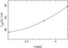 |
Fig. 2 Values of Teff / 100 and log (g) yielding equal abundances for Fe i and Fe ii. |
5. Anomalous saturation
The abundance from a set of equivalent widths of a given spectrum, e.g. Fe i, or Ti ii, should not, in principle, depend on the line strength. However, it has been known since the early days of curve of growth analysis, that drifts of abundance with line strength are common. They can result from a variety of causes ranging from errors in the oscillator strengths to equivalent width measurements. In a common situation, strong lines will give a higher abundance than weak ones, and the abundance worker can remove the trend by assuming an additional source of broadening known as microturbulence (ξt). This broadening arises from gas motions due to convection, mixing, or other sources not included in the basic expression for the absorption profile, such as hyperfine structure or Zeeman effect.
Plots of abundance vs. equivalent width for HD 101412 slope downward even when no microturbulence is assumed. Figure 3 shows the behavior for Ti ii lines. Not all plots show the flattening for weak lines. In particular, the Fe ii plot does not. However, most do.
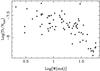 |
Fig. 3 log (Ti / Ntot) vs. log [ Wλ(mA) ] for Ti ii lines using the model with Teff = 8300 K, log (g) = 3.8. A microturbulence ξt = 0, was assumed. The downward trend of abundance with equivalent width illustrates the anomalous saturation. (Additional plots may be found at the URL given in Sect. 7.) |
An obvious mechanism that would weaken lines in young stars is veiling. This arises from excess continuum radiation arising from some aspect star-formation process (cf. Hartmann 2009). It is important to assess the possible effects of veiling, which would weaken the absorption lines and mimic lower abundances.
We believe the effect of veiling to be minor, for the following reasons:
-
Carbon, oxygen, and sulfur give abundances close to solar. In thecase of nitrogen, we find a significant excess. Veiling,if it were present, should have affected lines fromthese elements.
-
Veiling is often wavelength dependent. There is no indication of a drift in our abundances with wavelength for the five spectra having lines on either side of the Balmer jump: Mg I, V II, Cr I, Co I, and Co II.
-
Veiling is caused by an excess continuum due to infall from a disk. The veiling is less important for the Herbig Ae stars, relative to the T Tauri or weak T Tauri stars. There is no indication of X-rays from HD 101412, which would accompany significant infall of material.
We have found that anomalous saturation does not occur in a model with a hot upper atmosphere. If we arbitrarily raise the temperature from the standard ATLAS9 T(τ) the effect vanishes (see Fig. 4). Temperature changes were made by trial and error until the anomalous saturation was no longer evident in a plot of abundance from Fe II lines vs. equivalent width. The altered model is surely not unique. Since the results are from an LTE calculations, we take it as indicative of the problem with the ATLAS9 model for HD 101412 specifically. A realistic pursuit of this problem is best left to a NLTE study.
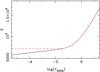 |
Fig. 4 Temperature distributions for the ATLAS9 model with Teff = 8300 K, log (g) = 3.8 (solid line), and a “hot top” model (dashed) which gives no anomalous saturation for ξt = 0. |
6. Teff – log (g) degeneracy; curves of growth
We can see from Fig. 2, and from Table 1, that higher temperatures require higher gravities. This is true for both the iron equilibrium and the Balmer profiles. The temperature (9500−10 000 K) obtained by earlier workers would not yield acceptable Fe ionization, though the Balmer lines could be accommodated with a higher surface gravity.
This leaves the question of how to break the degeneracy between temperature and gravity. In one of the relatively small number of abundance analyses of pre-main sequence stars, Acke & Waelkens (2004) determined atomic excitation temperatures “for ions with many observed lines”. Specifically, they required that the effective temperature of the model be such that there is no drift in the abundance determined from individual lines with excitation potential.
We have attempted to use the Acke & Waelkens (2004) method. Our results marginally favor a 8300 K − log (g) = 3.8 model over a 9800 K − log (g) = 4.2 model, though not decisively. The wrong temperature should show a clear difference between abundances from low- and high-excitation lines. Unfortunately anomalous saturation precluded use of many stronger lines, which are typically of low excitation. As we shall see, this was not a problem with the second method, based on a curve of growth technique.
Since our depth-dependent models are not accurate for this Herbig Ae star, it is worthwhile to explore results of a more basic approach where the photosphere is approximated by a uniform slab, with a single, mean value of the temperature and pressure. This simple technique was once widely used in the chemical analysis of stellar spectra, employing what were called Schuster-Schwarzschild (henceforth, SS) models. (cf. Aller 1963). The basic method is still routinely employed when the conditions along the line of sight are not well determined (cf. Spitzer 1978; Rachford et al. 2001; Hobbs 2005). This is the case for the upper layers of HD 101412.
Note: we use the SS models only to find an excitation temperature and break the Teff − log (g) degeneracy.
To determine an excitation temperature, we plot log (Wλ / λ) + 6 vs. log (gfλ) − θ·χ. Here, θ = 5040. / Texc, and χ is the lower excitation potential in eV. One adjusts the value of θ until the points belonging to lines with different excitation delineate, as well as possible, the same curve.
Constants are added to both the ordinates and abscissae of the observed points, in order to make the theoretical and stellar curves of growth overlap. The ordinate of the theoretical curve is log [ Wλ / (2r0ΔλD) ] , while that of the empirical plot is log (Wλ / λ) + 6. The vertical shift necessary to superimpose the two curves contains information on the Doppler width,  , and the maximum line depth r0, discussed in more detail below. The horizontal shift contains information on the column density, but that is not needed here. The analytical curves were originally due to van der Held (1931), and are are shown in the figure as solid lines for several values of the ratio of a = γλ / (2·ΔλD). Here γλ is the damping constant (in cm), μ is the molecular (atomic) weight, and ℛ the gas constant. Note that a constant has been added to our abscissa so that X and the ordinates of the theoretical curves are the same for weak lines. We made curves of growth for Ti ii, Fe i, and Fe ii, spectra with better-quality oscillator strengths, and Ca i We have tried to select oscillator strengths of optimum quality. Sources are:
-
Ti ii. Oscillator strengths are from Pickering et al.(2001).
-
Cr i. Oscillator strengths from Sobeck et al. (2007).
-
Cr ii. Oscillator strengths from Nilsson et al. (2006) or VALD (Kupka et al. 1999)/Kurucz (1994) taking only LS-permitted lines. Results were essentially the same.
-
Fe i. Lines from the NIST site (Ralchenko et al. 2010) with accuracy B+ (7 lines) and C+ (11 lines). Unfortunately, there are no lines with excitation potentials above 2.6 eV of accuracy B+ (see the NIST site for an explanation of “accuracy”).
-
Fe ii. We adopt the oscillator strengths of Meléndez & Barbuy (2009).
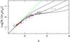 |
Fig. 5 Curve of growth for Fe ii lines using oscillator strengths from Meléndez & Barbuy (2009). Unit slope is indicated by the solid gray line. Along this line, the ordinate, and the abscissa (X), are equal. SS model curves are drawn for a = γλ / (2·ΔλD) of 1, 0.1, 0.01, and 0.001 (from the top). The abscissae for the points are log (gfλ) − θ·χ. Open circles are for 2.58 ≤ χ ≤ 2.89, open squares for 3.20 ≤ χ ≤ 3.89, and filled stars for 5.51 ≤ χ ≤ 6.22 eV. The observed points have been made to coincide by adding +5.7 to the abscissa, and −0.6 to the ordinate. The latter figure is relevant for the microturbulence. This plot was made with θ = 0.7 (7200 K). |
Figure 5 shows a curve of growth for Fe ii. Too large a θ (too low a temperature) will move the filled stars (highest χ) to the left with respect to the open circles (lowest χ). Too small a θ, would move the highest-χ points to the right. Points for the lowest-excitation lines move relatively little.
In the case of Ca i, there is no good recent set of oscillator strengths, apart from the three lines given by Aldenius et al. (2009), λλ6162.2, 6122.2, and 6102.7). These three lines are all of moderate strength (9.6 to 25.3 mÅ), and give −6.41, −6.42, and −6.30 for log (Ca / Ntot). We adopt −6.38; the mean of values from 35 lines is −6.43 ± 0.23 sd. A curve of growth is shown for Ca i in Fig. 6. Oscillator strengths for the remaining 32 lines are from the NIST site (Ralchenko et al. 2010).
Additional curves of growth and examples showing results of a wrong temperature may be found at the url given in Sect. 7.
Curves of growth provide a measure of the excitation temperature, the microturbulence (ξt), and the damping constant. The excitation temperatures found from the curves of growth, corresponding to θ = 0.65 to 0.7 (T = 7750 to 7200 K) are much cooler than any temperature discussed so far for HD 101412. However, the excitation temperature from the line spectrum is expected to be significantly lower than that from the continuum. We have made calculations based on model atmospheres to verify that the above excitation temperatures are to be expected for an atmosphere with Teff = 8300 K.
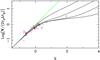 |
Fig. 6 Curve of growth for 35 Ca i lines. The resonance line, λ4227 is the open circle. Open squares are for the range 1.88 ≤ χ ≤ 1.90, triangles 2.50 ≤ χ ≤ 2.71, and filled stars (2 lines) 2.93 eV. Δx = 1.7 Δy = −0.65 and θ = 0.68 (T = 7410 K). Theoretical curves as in Fig. 5. |
The vertical displacement (Δy) necessary to superimpose the theoretical and empirical curves gives a relation between the maximum line depth r0, an assumed relevant temperature, and the microturbulence.
Our problem with the SS-model curves of growth is essentially the same as that with the ATLAS9 model. The maximum line depth expected for either model is too large, relative to the value needed in HD 101412 to give a finite microturbulence. In the case of the numerical model, r0 in LTE is simply ![Mathematical equation: $[1-B_\lambda(\tau_{\rm min})/(2F_0^c)]$](/articles/aa/full_html/2010/15/aa15361-10/aa15361-10-eq106.png) . The value, at λ4481 in the 8300 K − log (g) = 3.8 model is 0.90. For the SS model, if we adopt r0 = 0.53 from the observed λ4481 cores, and an excitation temperature of 7200 K, we find
. The value, at λ4481 in the 8300 K − log (g) = 3.8 model is 0.90. For the SS model, if we adopt r0 = 0.53 from the observed λ4481 cores, and an excitation temperature of 7200 K, we find  .
.
The strong lines in Fig. 5 fall between theoretical curves for the parameter a = γλ / (2·ΔλD) of 0.01 and 0.1. Note that γ (without a subscript) traditionally means γω, or the FWHM of a dispersion profile expressed as a function of ω = 2πc / λ.
Using T = 8300 K, and a mean λ = 4.6 × 10⁻⁵ cm, we obtain γ = 4.29 × 10⁹ s-1 for a = 0.1. This is 41 times the classical damping constant γcl = 0.22 / λ2 s-1 (with λ in cm). For a = 0.01, the result is 4 times the classical. A value commonly cited for the empirical damping constant is 10 times the classical value (cf. Mihalas 1970). Cowley & Cowley (1964) obtained γ / γcl = 25 for the sun. We thus see the value from this crude curve of growth is entirely reasonable for a star on or near, the main sequence.
7. Abundances
All abundances were determined from depth-dependent model calculations of equivalent widths assuming zero microturbulence. Oscillator strength references not explicitly mentioned are from NIST (Ralchenko 2010, preferred) or VALD (Kupka et al. 1999), except for Zr ii, where the values are from Ljung et al. (2006).
Plots of abundance vs. log (Wλ) were made for all species with more than three lines. Outliers could nearly always be understood and either corrected or dropped because of errors, such as misidentifications or blends. Whenever plots of abundance vs. equivalent widths exhibited a downward trend for stronger lines, abundances were determined from lines with equivalent widths ≤20 mÅ.
Additional plots were routinely made of abundance vs. excitation potential, and equivalent width vs. excitation potential. Our restriction to weak lines only for abundances eliminated most systematic effects, though some small effects are inevitable. Additional plots, and detailed line-by-line results are available from the first author or at the url: www.astro.umich.edu/~cowley/hd101412/.
Abundances are summarized in Table 2. Errors in Col. 3 are standard deviations for the number of lines used, or the difference in abundances when only 2 lines were available. For V i, the error is the difference from a single V i line, and the mean for V ii.
No exotic elements, were identified. Barium is the heaviest element positively identified, and the abundances listed for the lanthanides cerium and europium are upper limits. There was no indication of gallium or the heavier noble gases.
Adopted abundances.
Logarithmic abundance differences – star minus sun – are plotted in Fig. 7. The abundances may reflect a mild λ Boo, or Vega-like abundance mechanism, where the refractory elements are depleted while the most volatile elements are more nearly normal (Takeda 2008; see also Adelman et al. 2010, in prep.). This is not unexpected. Gray & Corbally (1998) classified the Herbig Ae star HD 37411 as a λ Boo star, while Acke & Waelkens (2004) describe the Herbig Ae star HD 100546 as a “clear λ Bootis star”, based on their abundance analysis.
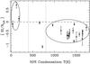 |
Fig. 7 Logarithmic abundance differences vs. 50%TC. Error bars are from Table 2. Volatile elements, C, N, O are enclosed within the ellipse on the left; refractory elements fall within the ellipse on the right. The intermediate volatiles, Zn and S, are between the dashed vertical lines. The decided outlier, Zn, is discussed in the text. |
Neither Vega nor HD 101412 would qualify as a λ Boo star, as they do not meet the 1 dex iron-peak deficiency of Paunzen (2004) for the λ Boo stars. Our average deficiency for the elements with 50%TC > 900 K is about 0.5 dex, half the depletion for classical λ Boo stars. Nor is there an obvious trend within these refractory elements with 50%TC.
Our suggestion that the abundance pattern resembles that of the λ Boo stars rests on average abundances for the elements with volatility extremes. The centroids of the ellipses in Fig. 7 are significantly displaced from one another, indicating the most volatile elements are not depleted while the most refractory elements are.
7.1. Outliers
The abundance pattern of Fig. 7 cannot be explained in terms of condensation temperature alone.
7.1.1. Nitrogen
The high nitrogen abundance may be partially due to NLTE. Kamp et al. (2001) find nitrogen quite variable among λ Boo stars, and subject to NLTE. For example, the LTE abundance excess of N for HD 75654 was +0.65 dex. The NLTE calculation reduced this value to +0.30 dex.
7.1.2. Sodium
Sodium (50%TC = 953 K), might be considered an intermediate volatile. We find its depletion in HD 101412 to be only 0.14 dex. However, Paunzen et al. (2002) reported sodium variations from −1.3 to +1.2 dex with respect to the sun. Kamp et al. (2008) discuss this further, and note mechanisms beyond equilibrium condensation that might account for the scatter.
7.1.3. Zinc
Paunzen (2004) listed zinc among the elements expected to be deficient in the λ Boo stars. To the extent that we suggest the abundances in HD 101412 resemble those of the λ Boo stars, our finding of an depletion of 1.06 dex ceases to indicate an outlier, and supports the assertion. At the same time, it complicates an interpretation based on volatility. Surely factors other than equilibrium condensation affect the stellar abundances of zinc as well as sodium.
8. Conclusions
The atmospheric structure of HD 101412 deviates from a classical model (e.g. ATLAS9). But the deeper photosphere, as probed by weaker lines, has a line spectrum well produced by the theoretical model with Teff = 8300 K, log (g) = 3.8. Elements with lines from the first and second spectra yield abundances in good or satisfactory agreement. In the worst case, silicon, Si i and Si ii disagree by 0.38 dex, only a factor of 2.4.
The atomic lines are also in general agreement with a mean excitation temperature in the range 7200 to 7750 K. An excitation temperature in this range is expected from a model with the adopted parameters.
Strong lines show an anomalous saturation, which we have attributed to maximum line depths, r0, less than that predicted by the ATLAS9 model. Similar information comes from curves of growth, where even the observed depths of the Mg ii λ4481 doublet (0.53) would lead to a imaginary value for the microturbulence.
Atomic emission features show departures of the upper atmosphere from classical. In addition to emissions seen in the low Balmer members, broad, generally weak emissions appear, for example, in [O i] λ6300, Na i D1 and D2, and the O i, triplet λλ7772, 7774, and 7775. The widths of these features are readily measured. The wavelength spread from the violet wing to the red wing, of atomic emissions correspond to velocities of 100 to 200 km s-1. We suggest the upper atmosphere is heated by infalling material from a primordial disk, and that this heating is probably responsible for the anomalous saturation.
Most abundances are less than 1 dex from solar values. With the notable exception of zinc, there is a suggestion that refractory elements are depleted. The volatiles are normal, or in the case of nitrogen, enhanced.
Acknowledgments
We are especially grateful to Z. Mikulášek for communicating the results of his photometric period in advance of publication and for an exchange of ideas concerning its interpretation. It is a pleasure to thank J. R. Fuhr J. Reader, and W. Wiese of NIST for advice on atomic data and processes. This research has made use of the SIMBAD database, operated at CDS, Strasbourg, France. Our calculations have made extensive use of the VALD atomic data base (Kupka et al. 1999). C.R.C. is grateful for advice and helpful conversations with many of his Michigan colleagues, and to Jesús Hernández for useful comments and suggestions. S. J. Adelman and A. F. Gulliver graciously shared some results of their forthcoming Vega abundance study.
References
- Acke, B., & Waelkens, C. 2004, A&A, 427, 1009 [NASA ADS] [CrossRef] [EDP Sciences] [Google Scholar]
- Aldenius, M., Lundberg, H., & Blackwell-Whitehead, R. 2009, A&A, 502, 989 [NASA ADS] [CrossRef] [EDP Sciences] [Google Scholar]
- Aller, L. H. 1963, Astrophysics, The Atmospheres of the Sun and Stars, 2nd edn. (New York: Ronald Press Co.) [Google Scholar]
- Asplund, M., Grevesse, N., Sauval, A. J., & Scott, P. 2009, ARA&A, 47, 481 [NASA ADS] [CrossRef] [Google Scholar]
- Castelli, F. 2010, wwwuser.oat.ts.astro.it/castelli/grids.html [Google Scholar]
- Castelli, F., & Hubrig, S. 2004, A&A, 421, L1 [NASA ADS] [CrossRef] [EDP Sciences] [Google Scholar]
- Castelli, F., & Kurucz, R. L. 2003, in Modelling of Stellar Atmospheres, ed. N. Piskunov, W. W. Weiss, & D. F. Gray, IAU Symp., 210, 424 [Google Scholar]
- Cowley, C. R., & Cowley, A. P. 1964, ApJ, 140, 713 [NASA ADS] [CrossRef] [Google Scholar]
- Cox, A. N. 2000, Allen’s Astrophysical Quantities, 4th edn. (Berlin: Springer) [Google Scholar]
- Fedele, D., van den Ancker, M. E., Acke, B., et al. 2008, A&A, 491, 809 [NASA ADS] [CrossRef] [EDP Sciences] [MathSciNet] [Google Scholar]
- Gray, R. O., & Corbally, C. J. 1998, AJ, 116, 2530 [NASA ADS] [CrossRef] [Google Scholar]
- Guimarães, M. M., Alencar, S. H. P., Corradi, W. J. B., & Vieira, S. L. A. 2006, A&A, 457, 581 [NASA ADS] [CrossRef] [EDP Sciences] [Google Scholar]
- Hartmann, L. 2009, Accretion Processes in Star Formation, 2nd edn. (Cambridge: University Press) [Google Scholar]
- Hernández, J., Calvet, N., Hartmann, L., et al. 2005, AJ, 129, 856 [NASA ADS] [CrossRef] [Google Scholar]
- Hobbs, L. M. 2005, MNRAS, 359, 1356 (see Sect. 2.2 and Fig. 1) [NASA ADS] [CrossRef] [Google Scholar]
- Houk, N., & Cowley, A. P. 1975, The University of Michigan Catalogue of Two-Dimensional Spectral Types for the HD Stars, Vol. I, Dept. of Astron: Univ. of Michigan [Google Scholar]
- Hubrig, S., Kurtz, D. W., Bagnulo, S., et al. 2004, A&A, 415, 661 [NASA ADS] [CrossRef] [EDP Sciences] [Google Scholar]
- Hubrig, S., Stelzer, B., Schöller, M., et al. 2009, A&A, 283, 2009 [Google Scholar]
- Hubrig, S., Schöller, M., Savanov, I., et al. 2010, AN, 331, 361 [Google Scholar]
- Kamp, I., Iliev, I. Kh., Paunzen, E., et al. 2001, A&A, 375, 899 [NASA ADS] [CrossRef] [EDP Sciences] [Google Scholar]
- Kamp, I., Martínez-Galarza, J. R., Paunzen, E., et al. 2008, CoSka, 38, 147 [NASA ADS] [Google Scholar]
- Kupka, F., Piskunov, N. E., Ryabchikova, T. A., Stempels, H. C., & Weiss, W. W. 1999, A&AS, 138, 119 [NASA ADS] [CrossRef] [EDP Sciences] [MathSciNet] [PubMed] [Google Scholar]
- Kurucz, R. L. 1993, ATLAS9 Stellar Atmosphere Programs and 2 km s-1 grid, CD-Rom, No. 13, Cambridge MA: Smithsonian Ap. Obs. [Google Scholar]
- Kurucz, R. L. 1994, Atomic Data for Ca–Ni, CD-Roms, Nos. 20−22, Cambridge MA: Smithsonian Ap. Obs. [Google Scholar]
- Ljung, G., Nilsson, H., Asplund, M., & Johansson, S. 2006, A&A, 456, 1181 [NASA ADS] [CrossRef] [EDP Sciences] [Google Scholar]
- Lodders, K. 2003, ApJ, 591, 1220 [NASA ADS] [CrossRef] [Google Scholar]
- Meeus, G., Waters, L. B. F. M., Bouwman, J., et al. 2001, A&A, 365, 476 [NASA ADS] [CrossRef] [EDP Sciences] [Google Scholar]
- Meléndez, J., & Barbuy, B. 2009, A&A, 497, 611 [NASA ADS] [CrossRef] [EDP Sciences] [Google Scholar]
- Mermilliod, J.-C., Hauck, B., & Mermilliod, M. 2007, General Catalogue of Photometric Data, http://www.unige.ch/sciences/astro [Google Scholar]
- Mihalas, D. 1970, Stellar Atmospheres, 1st edn. (San Francisco: W. H. Freeman), see p. 340 [Google Scholar]
- Nilsson, H., Ljung, G., Lundberg, H., & Nielson, K. E. 2006, A&A, 445, 1165 [NASA ADS] [CrossRef] [EDP Sciences] [Google Scholar]
- Paunzen, E. 2004, in The A Star Puzzle, IAU Symp., 224, 443 [Google Scholar]
- Paunzen, E., Iliev, I. Kh., Kamp, I., & Barzova, I. S. 2002, MNRAS, 336, 1030 [NASA ADS] [CrossRef] [Google Scholar]
- Pickering, J. C., Thorne, A. P., & Perez, R. 2001, ApJS, 132, 403 (Erratum: ApJS, 138, 247, 2002) [NASA ADS] [CrossRef] [Google Scholar]
- Rachford, B. L., Snow, T. P., Tumlinson, J., et al. 2001, ApJ, 555, 839 (see Figs. 4 and 5) [NASA ADS] [CrossRef] [Google Scholar]
- Ralchenko, Yu., Kramida, A. E., Reader, J., & NIST ASD Team 2010, NIST Atomic Spectra Database (version 3.1.5), [Online] Available: http://physics.nist.gov/as of [2010, Feb. 10], National Institute of Standards and Technology, Gaithersburg, MD. [Google Scholar]
- Sbordone, L., Bonifacio, P., Castelli, F., & Kurucz, R. L. 2004, Mem. S. A. It. Suppl., 5, 93 [Google Scholar]
- Sobeck, J. S., Lawler, J. E., & Sneden, C. 2007, ApJ, 667, 1267 [NASA ADS] [CrossRef] [Google Scholar]
- Spitzer, L., Jr. 1978, Physical Processes in the Interstellar Medium (New York: J. Wiley &Sons), cf. Chapt. 3 [Google Scholar]
- Takeda, Y. 2008, MNRAS, 388, 913 [NASA ADS] [CrossRef] [Google Scholar]
- van der Held, E. F. M. 1931, Zs. f. Physik, 70, 508 [Google Scholar]
- Venn, K. A., & Lambert, D. L. 1990, ApJ, 363, 234 [NASA ADS] [CrossRef] [Google Scholar]
- Vieira, S. L. A., Corradi, W. J. B., Alencar, S. H. P., et al. 2003, AJ, 126, 2971 [NASA ADS] [CrossRef] [Google Scholar]
- Wade, G. A., Drouin, D., Bagnulo, S., et al. 2005, A&A, 442, L31 [NASA ADS] [CrossRef] [EDP Sciences] [Google Scholar]
All Tables
Provisional abundances (log (Fe / Ntot)) from Fe i and Fe ii for various temperatures and surface gravities.
All Figures
|
Fig. 1 Hβ (above, top wavelength scale) and Hδ profiles (bottom wavelength scale) for Teff = 8300 K, log (g) = 3.8 and 9800 K, log (g) = 3.8. Observed profiles are in gray (red in online version) with dots. The fits for the lower temperature are as good or arguably better than at the higher temperature. The relative flux scale is correct for the lowest profile pair. Upper pairs are successively raised by 0.4 units. |
| In the text | |
|
Fig. 2 Values of Teff / 100 and log (g) yielding equal abundances for Fe i and Fe ii. |
| In the text | |
|
Fig. 3 log (Ti / Ntot) vs. log [ Wλ(mA) ] for Ti ii lines using the model with Teff = 8300 K, log (g) = 3.8. A microturbulence ξt = 0, was assumed. The downward trend of abundance with equivalent width illustrates the anomalous saturation. (Additional plots may be found at the URL given in Sect. 7.) |
| In the text | |
|
Fig. 4 Temperature distributions for the ATLAS9 model with Teff = 8300 K, log (g) = 3.8 (solid line), and a “hot top” model (dashed) which gives no anomalous saturation for ξt = 0. |
| In the text | |
|
Fig. 5 Curve of growth for Fe ii lines using oscillator strengths from Meléndez & Barbuy (2009). Unit slope is indicated by the solid gray line. Along this line, the ordinate, and the abscissa (X), are equal. SS model curves are drawn for a = γλ / (2·ΔλD) of 1, 0.1, 0.01, and 0.001 (from the top). The abscissae for the points are log (gfλ) − θ·χ. Open circles are for 2.58 ≤ χ ≤ 2.89, open squares for 3.20 ≤ χ ≤ 3.89, and filled stars for 5.51 ≤ χ ≤ 6.22 eV. The observed points have been made to coincide by adding +5.7 to the abscissa, and −0.6 to the ordinate. The latter figure is relevant for the microturbulence. This plot was made with θ = 0.7 (7200 K). |
| In the text | |
|
Fig. 6 Curve of growth for 35 Ca i lines. The resonance line, λ4227 is the open circle. Open squares are for the range 1.88 ≤ χ ≤ 1.90, triangles 2.50 ≤ χ ≤ 2.71, and filled stars (2 lines) 2.93 eV. Δx = 1.7 Δy = −0.65 and θ = 0.68 (T = 7410 K). Theoretical curves as in Fig. 5. |
| In the text | |
|
Fig. 7 Logarithmic abundance differences vs. 50%TC. Error bars are from Table 2. Volatile elements, C, N, O are enclosed within the ellipse on the left; refractory elements fall within the ellipse on the right. The intermediate volatiles, Zn and S, are between the dashed vertical lines. The decided outlier, Zn, is discussed in the text. |
| In the text | |
Current usage metrics show cumulative count of Article Views (full-text article views including HTML views, PDF and ePub downloads, according to the available data) and Abstracts Views on Vision4Press platform.
Data correspond to usage on the plateform after 2015. The current usage metrics is available 48-96 hours after online publication and is updated daily on week days.
Initial download of the metrics may take a while.