| Issue |
A&A
Volume 523, November-December 2010
|
|
|---|---|---|
| Article Number | A83 | |
| Number of page(s) | 6 | |
| Section | Cosmology (including clusters of galaxies) | |
| DOI | https://doi.org/10.1051/0004-6361/201014385 | |
| Published online | 18 November 2010 | |
The dark matter density at the Sun’s location
1
SISSA/ISAS, via Beirut 2-4,
34013
Trieste,
Italy
e-mail: This email address is being protected from spambots. You need JavaScript enabled to view it.
2
Dipartimento di Fisica, Università di Ferrara,
44100
Ferrara,
Italy
3
Institut d’Astronomie et d’Astrophysique, Université Libre de
Bruxelles, CP 226, Bvd du Triomphe, 1050 Bruxelles, Belgium,
Sterrenkundig Observatorium, Universiteit Gent, Krijgslaan 281, 9000
Gent,
Belgium
4
Universidade Federal do ABC, Rua Catequese 242, 09090-400
Santo André-São Paulo,
Brasil
Received:
8
March
2010
Accepted:
17
June
2010
Abstract
Aims. We derive the value of the dark matter density at the Sun’s location (ρ⊙) without fully modeling the mass distribution in the Galaxy.
Methods. The proposed method relies on the local equation of centrifugal equilibrium and is independent of i) the shape of the dark matter density profile, ii) knowledge of the rotation curve from the galaxy center out to the virial radius, and iii) the uncertainties and the non-uniqueness of the bulge/disk/dark halo mass decomposition.
Results. The result can be obtained in analytic form, and it explicitly includes the dependence on the relevant observational quantities and takes their uncertainties into account. By adopting the reference, state-of-the-art values for these, we find ρ⊙ = 0.43(11)(10) GeV/cm3, where the quoted uncertainties are respectively due to the uncertainty in the slope of the circular-velocity at the Sun location and the ratio between this radius and the length scale of the stellar exponential thin disk.
Conclusions. We obtained a reliable estimate of ρ⊙, that, in addition has the merit of being ready to take any future change/improvement into account in the measures of the observational quantities it depends on.
Key words: Galaxy: kinematics and dynamics / dark matter
© ESO, 2010
1. Introduction
Galaxy rotation curves (e.g. Rubin et al. 1980; Bosma et al. 1981) have unveiled a dark “mass component” in spirals. They are pillars of the paradigm of massive dark halos, composed of a still undetected kind of matter surrounding the luminous part of galaxies. The kinematics of spirals shows universal systematics (Persic & Salucci 1996; Salucci et al. 2007), which seems to be at variance with the predictions emerging from simulations performed in the Λ cold dark matter (ΛCDM) scenario, (e.g. Navarro et al. 1996), the currently preferred cosmological paradigm of galaxy formation (e.g. Gentile et al. 2004). Individual and coadded rotation curves (RCs) of spiral galaxies are also crucial to investigate frameworks alternative to the standard paradigm of cold collisionless DM in Newtonian gravity (e.g. Sanders & McGaugh 2002; Berezhiani et al. 2009,b).
At the same time, dedicated searches of DM particle candidates have seen an important boost in recent years with relevant and costly experiments being planned and executed. The so-called direct-detection experiments look for the scattering of DM particles off the nuclei inside the detectors (e.g. CDMS, XENON10, DAMA/LIBRA) by typically measuring the deposited energy or its annual modulation. Clearly in all these experiments the signal is proportional to the DM density in the Sun’s region, ρ⊙. On the other hand indirect-detection experiments (in particular Super-Kamionkande, AMANDA, IceCube and ANTARES) search for the secondary particles (neutrinos in these cases) produced by DM annihilations at the center of the Sun or Earth, where it is expected that DM accumulates after losing energy via scattering, possibly reaching a thermalized state. The expected signal in this case depends on the DM density inside these objects, which in turn is driven, via the capture mechanism, by the same halo DM density in the Sun region, ρ⊙. Therefore, in both these kinds of direct and indirect searches, an estimate of the the local density ρ⊙ is very important for a precise estimate of the signal or at least reliable bounds on the DM cross-section vs mass to be compared with limits from other searches.
What is then the value of ρ⊙? A value of  (1)is routinely quoted in hundreds of papers, but how does this number come out? In which works do we find the details of its measure? It is worth observing that in most of the cases in the literature, the above value is given with no reference (e.g. Donato et al. 2009; Savage et al. 2009). Sometimes, the reference goes to a couple of seminal papers. Among them, the Particle Data Group Review (PDG 2008) indicates the above value “within a factor of two or so” and justifies it as coming from “recent estimates based on a detailed model of our Galaxy”. However, the works cited are neither recent nor detailed and sometimes not even an independent estimation of ρ⊙.
The only exception is the work by Caldwell & Ostriker (1981) that devised what can be considered as the standard method (CO hereafter) to determine the value of ρ⊙ from observations (see below). Their resulting value,  GeV/cm3, arises however from very outdated kinematical observations and from a cored (rather than a cuspy) halo distribution, so it is not a great support for Eq. (1). Similar conclusions can be drawn by looking at other influential reviews: the papers they cite to back up the value (1) either do not estimate this quantity or use very outdated observations.
In general, it is quite simple to infer the distribution of dark matter in spiral galaxies. Spiral’s kinematics, in fact, reliably traces the underlying gravitational potential (Persic & Salucci 1996; Salucci et al. 2007). Then, from coadded and/or individual RCs, we can build suitable global models of the mass distributions that include stellar and gaseous disks along with a spherical bulge and a dark halo. More in detail, by carefully analyzing (high quality) circular velocity curves, with the help of relevant photometric and HI data, one can derive the halo density at any desired radius. The accuracy of the “measurements” is excellent and the results are at the core of the present debates on Galaxy formation (e.g. Gentile et al. 2004, 2005; DeBlok 2010).
To measure ρ⊙, instead, is far from simple, because the MW kinematics, unlike that of external galaxies, does not trace the gravitational potential straightforwardly. We do not directly measure the circular velocity of stars and gas but rather, at our best, the terminal velocity VT of the rotating HI disk, and this only inside the solar circle (e.g. McClure-Griffiths & Dichey 2007). This velocity is related to the circular velocity V(r), for r < R⊙, by means of V(r) = VT(r) + V⊙ r / R⊙, where R⊙ ≃ 8 kpc is the distance of the Sun from the Galaxy center and V⊙ the value of the circular velocity at the Sun’s position. Both quantities are known within an uncertainty of 5%−10% (e.g. McMillan & Binney 2010), which triggers a similar uncertainty in the derived magnitude and slope of the circular velocity.
As a result, and also considering other kinematical observations (see Sofue 2009), the circular velocity of the MW from 2 to 8 kpc can be only derived within non negligible uncertainties: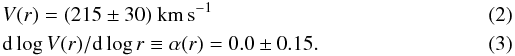 \arraycolsep1.75ptNote that the range of circular velocities in Eq. (2) is created by a mix of a) observational errors; b) uncertainties in the values of R⊙ and V⊙; and c) actual radial variations of V. The first two trigger also part of the range of the velocity slope (3). We stress that data show that the radial variations of α(r) are small and likely caused by the uncertainties just discussed: in either case we have dα(r) / dr ≃ 0 ± 0.03 / kpc ≃ 0. In other words, in this region the RC can be approximated by a straight line, whose slope is known however only within a degree of uncertainty.
The outer (out to 60 kpc) MW “effective” circular velocity V(r) = (GM(r) / r)1 / 2 is, instead, much more uncertain and depends on the assumptions made on dynamical and structural properties of its estimators. It appears to decline with radius, with quite an uncertain slope (Battaglia 2005; Xue et al. 2008; Brown et al. 2010)  (4)These uncertainties, combined with the intrinsic “flatness” of the RC in the region specified above (that complicates the mass modeling even in the case of a high-quality, RC, Tonini & Salucci 2004), make it very difficult to obtain a reliable bulge/disk/halo mass model and consequently an accurate estimate of ρ⊙.
To overcome these serious difficulties Caldwell & Ostriker (1981) developed a method in which other observational data, linked in various ways to the gravitational potential, help with the mass modeling. These include the l.o.s. dispersion velocities of bright tracers at known distances from the Sun (e.g. OB stars) and the total Galaxy mass. This extra information allows a determination of ρ⊙, though it turns out to be uncertain within a factor 2 (Caldwell & Ostriker 1981), or somewhat less when more constraints from the z motions of disk stars are added (e.g. Olling & Merrifield 2001; Weber & de Boer 2010; Sofue 2009)1.
By averaging the results from different determinations obtained so far, one finds ρ⊙ = (0.3 ± 0.2) GeV / cm3, where the uncertainty in the result is triggered in an unspecified way from observational and fitting uncertainties, as from biases arising from the various assumptions taken by the method, not the least the assumed DM density profile.
Recently, by applying the CO method with a refined statistical analysis to a large set of observational data, Catena & Ullio (2010) claimed a measure with a very small uncertainty: ρ⊙ = (0.389 ± 0.025) GeV/cm3. While this result would be noticeable, it has not been confirmed by a subsequent work (Weber & de Boer 2010) and it seems unlikely, in view of Eqs. (2) and (3), reflecting the state of art of our (lack of) knowledge.
The aim of this work is to derive ρ⊙ by following a more direct route than mass modeling the whole Galaxy and dynamically modeling a number of galactic components and a series of galactic potential tracers. This will be done by means of a specifically devised method and by using some recent results obtained for external galaxies (Salucci et al. 2007). The idea is to resort to the equation of centrifugal equilibrium, holding in spiral galaxies (see Fall & Efstathiou 1980, for details) 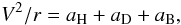 (5)where aH, aD, and aB are the radial accelerations generated by the halo, stellar disk, and bulge mass distributions. Taking first the (quite good) approximation of spherical DM halo, we have
 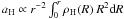 . A similar relation holds for the bulge. Therefore, by differentiating Eq. (5), we obtain the DM density at any radius in terms of the local angular velocity ω(r) = V / r, the RC slope α(r), the disk-to-dynamical mass ratio β(r) (see later), and the bulge mass density:
 ![Mathematical equation: \begin{equation} \label{eq:rhoDM1} \rho_{\rm H} (r) = \omega(r)^2 \left[F_{\rm tot}(\alpha(r)) - F_{\rm D} (\beta(r)\right]-\rho_{\rm B}(r). \end{equation}](/articles/aa/full_html/2010/15/aa14385-10/aa14385-10-eq34.png) (6)with Ftot and FD known functions.
(6)with Ftot and FD known functions.
In spirals, Eq. (6) is not useful for determining the DM density at any radius because 1) it virtually collapses for r < RD where Ftot ≃ FD, and the bulge density can also become dominating, ρB ≫ ρH; 2) the radial variations of α(r) have non-negligible observational uncertainty that further complicates the effect discussed in the previous point; 3) the quantity ω is known with less accuracy than V, the observational quantity entering the traditional mass modeling.
Instead, in estimating ρ⊙, i.e. the density of the MW DM halo at a specific radius (the Sun position), the above drawbacks disappear: 1) since R⊙ > 3RD we have Ftot(R⊙) ≫ FD(R⊙), Eq. (6) does not collapse and, as a bonus, the most uncertain term of the rhs of (6) is also the smaller one; 2) ω⊙ is very precisely measured; 3) dα / dr | R⊙ ≃ 0; and 4) at the Sun’s position the bulge density ρB(R⊙) is totally negligible, < ρH / 50 (e.g. Sofue et al. 2009). Thus, this method is very powerful for determining the value of the DM density at R⊙. The DM density at any radii is obviously left to the standard mass modeling.
The method is obviously simpler for a spherically symmetric DM halo, and can be further simplified by considering an infinitesimally thin disk for the distribution of stars in the Galaxy. However, below we also include the effects of a possible halo oblateness and disk thickness. Here, we anticipate that these effects, constrained by observations, are rather weak, of the order of a few percent, and are therefore irrelevant for this work. As a result, we obtain a reliable and model-independent determination of the local DM halo density, as well as of its intrinsic uncertainty.
In the next section we describe the method in detail and derive ρ⊙ and its uncertainty as a function of the relevant observables. In the last section we discuss the results and draw the conclusions. In the Appendices, we explicitly describe the effect of the halo oblateness and disk thickness, and we comment on the inherent problems in the traditional determination of ρ⊙.
2. A model-independent method
We model the Galaxy as composed by a stellar exponential thin disk (Freeman 1970), plus an unspecified spherical DM halo with density profile ρH(r). For the present work we can neglect the HI disk because its surface density, between 2 kpc and R⊙, is 100 to 5 times smaller than the stellar surface density (Nakanishi & Sofue 2003). Similarly, we neglect the stellar bulge because, as mentioned above, its spatial density at R⊙ is virtually zero (e.g. Sofue et al. 2009). The standard method and its variants cannot take these very simplifying assumptions because modeling the mass distribution of the Galaxy involves these mass components in a crucial way.
As discussed in the introduction we can rewrite the equation of centrifugal equilibrium by subtracting the disk component from the total acceleration. From its radial derivative we then find ![Mathematical equation: \begin{equation} \rho_{\rm H}(r) = \frac{X_q}{4 \pi G r^2}\, \frac{{\rm d}}{{\rm d}r} \left[r^2\left(\frac{V^2(r)}{r} - a_{\rm D}(r)\right)\right], \label{eq:rhohalo} \end{equation}](/articles/aa/full_html/2010/15/aa14385-10/aa14385-10-eq50.png) (7)where Xq is a factor correcting the spherical Gauss law used above in case of oblateness q of the DM halo.
(7)where Xq is a factor correcting the spherical Gauss law used above in case of oblateness q of the DM halo.
We describe the factor Xq in Appendix A. Since the observational evidence for an oblateness of the Galactic DM halo is still quite uncertain and at the same time the mean value of q, as measured in a very large sample of external spirals, is very near to 1 (see e.g. O’Brien et al. 2010, for a recent review of this issue), we consider q = 0.95 ± 0.05 here as the reference value and compute Xq accordingly (see Appendix A). We thus find that from present observations Xq boils down to a correction of less than 5% to ρ⊙, Xq ≃ 1.00−1.05. Let us stress that by means of Eq. (A.1) one may also take into account a value of q, emerging from future improved observations, outside the range considered here.
The disk component can be reliably modeled as a Freeman stellar exponential thin disk of length scale (Picaud & Robin 2004; Jurić et al. 2008; Robin et al. 2008; Reylé 2009) RD = (2.5 ± 0.2) kpc. The stellar surface density is then:  . Also, the disk can be considered infinitesimally thin. In fact, its thickness z0 is small, z0 ~ 250 pc (Jurić et al. 2008) and moreover z0 ≪ RD < R⊙, so that its effect on the derivative of the acceleration, and in turn on our measure, is very limited. For the sake of completeness, we compute it explicitly in Appendix B and show that it implies a reduction of less than 5% of the aD term as computed for an infinitesimally thin disk. We can thus write
  , where In and Kn are the modified Bessel functions computed at r / 2RD, and Xz0 ≃ 0.95 accounts for the nonzero disk thickness (See Appendix B).
Since only the first derivative of the circular velocity V(r) enters in (7) and in any case this function in the solar neighborhood is almost linear, we can write ![Mathematical equation: \begin{equation} V(r) = V_{\odot} \left[1 + \alpha_\odot\, \left(r-R_\odot\right)/R_\odot\right], \end{equation}](/articles/aa/full_html/2010/15/aa14385-10/aa14385-10-eq65.png) (8)where α⊙ = α(R⊙) is the velocity slope at the Sun’s radius. Then Eq. (7) becomes
(8)where α⊙ = α(R⊙) is the velocity slope at the Sun’s radius. Then Eq. (7) becomes ![Mathematical equation: \begin{equation} \label{rhoh} \rho_{\rm H}(r) = \frac{X_q}{4 \pi G}\left[\frac{V^2(r)}{r^2} \left(1+2 {\alpha_\odot}\right) - \frac{GM_{\rm D}}{R_{\rm D}^3} H\left(r/R_{\rm D}\right)\,X_{z_0}\right], \end{equation}](/articles/aa/full_html/2010/15/aa14385-10/aa14385-10-eq67.png) (9)with 2H(r / RD) = (3I0K0 − I1K1) + (r / RD)(I1K0 − I0K1). Equation (9) holds at any radius outside the bulge region and measures ρH(R⊙) ≡ ρ⊙ by subtracting the “effective” density of the stellar component from the one of all the gravitating matter.
(9)with 2H(r / RD) = (3I0K0 − I1K1) + (r / RD)(I1K0 − I0K1). Equation (9) holds at any radius outside the bulge region and measures ρH(R⊙) ≡ ρ⊙ by subtracting the “effective” density of the stellar component from the one of all the gravitating matter.
The disk mass can be parametrized (Persic & Salucci 1990b) by  , with
  , i.e. the fraction of the disc contribution to the circular velocity at the Sun.
Finally, by exploiting the fact that the quantity V / R | R⊙ ≡ ω = (30.3 ± 0.3) kms-1 / kpc is measured with very high accuracy and much better than V⊙ and R⊙ separately (McMillan & Binney 2010; Reid 2009), and after defining r⊙D ≡ R⊙ / RD, we obtain ![Mathematical equation: \begin{eqnarray} \label{rhoodot} \rho_\odot &=& 1.2 \times 10^{-27} {\rm \frac{g}{cm^3}}\left(\frac{\omega}{{\rm km\,s^{-1}\,kpc}}\right)^2 X_q\big[ \left(1 + 2{\alpha_\odot}\right)\nonumber\\ && - 1.1 \,\beta \, f\left(r_{\odot {\rm D}}\right)\, X_{z_0} \big], \end{eqnarray}](/articles/aa/full_html/2010/15/aa14385-10/aa14385-10-eq74.png) (10)where
(10)where  .
.
It is now possible to observe the advantages of the proposed method: a) it does not require assuming a particular DM halo density profile, or the dynamical status of some distant tracers of the gravitational field; b) it is independent of the (poorly known) values of V⊙ and of the RC slope at different radii; c) it does not depend on the structural properties of the bulge, which in the mass modeling creates a degeneration with the stellar disk and DM halo. d) it only mildly depends on the ratio r⊙D, as well as on the disk mass parameter β; finally, e) the method depends on the RC slope at the Sun α⊙, although in a specified way. In all points a) − e) the method brings an evident improvement over the CO one.
To proceed further we discuss the parameters appearing in Eq. (10). Our determination does not depend on the value of R⊙ and RD separately, but only on their ratio r⊙D. For this we adopt the reference value and uncertainty r⊙D = 3.4 ± 0.52, as suggested by the values of RD given above and by the average of values of R⊙ obtained in recent works R⊙ = 8.2 ± 0.5 kpc (Ghez et al. 2008; Gillessen et al. 2008; Bovy et al. 2009). This leads to f(r⊙D) ≃ 0.42 ± 0.20, whose uncertainty propagates only mildly into the determination of ρ⊙, because the second term of the rhs of Eq. (10) is only one third of the value of the first. (And it can only reach one half by stretching all other uncertainties.)
Present data constrain the slope of the circular velocity at the Sun to a central value of α⊙ = 0 and within a fairly narrow range −0.075 ≤ α⊙ ≤ 0.075. The uncertainty of α⊙ is the main source of the uncertainty of the present determination of ρ⊙, and let us recall that also values outside our adopted range may be used in the present analytic determination, for instance, a value belonging to a wider range allowed for α⊙ claimed by (Olling & Merrifield 2001).
In Eq. (10), β is the only quantity that is not observed and therefore intrinsically uncertain. We can, however, constrain it by computing the maximum value βM for which the disk contribution at 2.2RD (where it has its maximum) totally accounts for the circular velocity. With no assumption on the halo density profile one gets βM = 0.85, independently of V⊙ and R⊙ (Persic & Salucci 1990b). However, this is really an absolute maximal value and it corresponds, out to R⊙, to a solid body halo profile: Vh ∝ Rαh with αh = 1. Instead, all mass modeling performed so far for the MW and for external galaxies have found a lower value αh(3RD) ≤ 0.8, which yields βM = 0.77. We can also set a lower limit for the disk mass, i.e. βm: first, the microlensing optical depth to Baade’s Window constrains the baryonic matter within the solar circle to be greater than 3.9 × 10¹⁰ M⊙ (McMillan & Binney 2010). Moreover, the MW disk B-band luminosity LB = 2 × 10¹⁰ L⊙ coupled with the very reasonable value MD / LB = 2 again implies MD ≃ 4 × 10¹⁰ M⊙. All this implies βm = βM / 1.3 ≃ 0.653. We thus take  as reference range.
Using the reference values, we get ![Mathematical equation: \begin{eqnarray} \rho_{\odot} &=& 0.43 {\rm \frac{GeV}{cm^3}}\bigg[1 + 2.9\,{\alpha_\odot} -0.64\, \left(\beta-0.72\right) + 0.45\left(r_{\odot {\rm D}}-3.4\right) \nonumber\\ && - 0.1\left(\frac{z_0}{{\rm kpc}}-0.25\right)+ 0.10 \left(q-0.95\right)\nonumber\\ && + 0.07\left(\frac{\omega}{\rm km\,s^{-1}\,kpc}-30.3\right)\bigg]. \label{eq:10bis} \end{eqnarray}](/articles/aa/full_html/2010/15/aa14385-10/aa14385-10-eq102.png) (11)This equation, which is the main result of our paper, estimates the DM density at the Sun’s location in an analytic way, in terms of the involved observational quantities at their present status of knowledge. The equation is written in a form such that, for the present reference values of these quantities, the term in the square brackets on the rhs equals 1, so that the central result is ρ⊙ = 0.43 GeV/cm3. As such, the determination is ready to account for future changes, improved measurement or any choice of α⊙, β, z0, ω, r⊙D, q different from the reference values adopted here, by simply inserting them in the rhs of Eq. (11).
(11)This equation, which is the main result of our paper, estimates the DM density at the Sun’s location in an analytic way, in terms of the involved observational quantities at their present status of knowledge. The equation is written in a form such that, for the present reference values of these quantities, the term in the square brackets on the rhs equals 1, so that the central result is ρ⊙ = 0.43 GeV/cm3. As such, the determination is ready to account for future changes, improved measurement or any choice of α⊙, β, z0, ω, r⊙D, q different from the reference values adopted here, by simply inserting them in the rhs of Eq. (11).
The next step is to estimate the uncertainty in the present determination of ρ⊙, which is triggered entirely by the uncertainties of the quantities entering the determination. From Eq. (11) and the allowed range of values discussed above, we see that the main sources of uncertainty are α⊙, β and r⊙D, which appear in the first line. The other parameters give at most variations of 2−3%, and can be neglected in the following.
Then, first, it is illustrative to consider α⊙, β and r⊙D as independent quantities. We thus have: 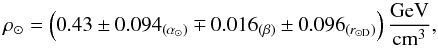 (12)where A(x) means that A is the total effect due to the possible span of the quantity x.
At this point, we can go one step further, assuming that the MW is a typical spiral, and using recent results for the distribution of matter in external galaxies, namely that DM halos around spirals are self similar (Salucci et al. 2007) and that the fractional amount of stellar matter β shapes the rotation curve slope α⊙ (Persic & Salucci 1990b):  (13)Using this relation in Eq. (11) we find (neglecting the irrelevant q and z0 terms)
 ![Mathematical equation: \begin{eqnarray} \label{eq:11bis} \rho_{\odot} &=& 0.43 {\rm \frac{GeV}{cm^3}}\bigg[1 + 3.5\,{\alpha_\odot} + 0.45\left(r_{\odot {\rm D}}-3.4\right) \nonumber\\ && + 0.07\left(\frac{\omega}{\rm km\,s^{-1}\,kpc}-30.3\right)\bigg]. \end{eqnarray}](/articles/aa/full_html/2010/15/aa14385-10/aa14385-10-eq110.png) (14)From the current known uncertainties, with the estimated range of α⊙, we find
(14)From the current known uncertainties, with the estimated range of α⊙, we find  (15)This is our final estimate, which is somewhat higher than previous determinations. Its uncertainty mainly reflects our poor knowledge of the velocity slope α⊙ and the uncertainty in the galactocentric Sun distance.
3. Discussion and conclusion
In this work we have provided a model-independent kinematical determination of ρ⊙. The method proposed here derives ρ⊙ directly from the solution of the equation of centrifugal equilibrium, by estimating the difference between the “total” density and that of the stellar component.
The method leads to an optimal kinematical determination of ρ⊙, avoiding model-dependent and dubious tasks mandatory with the standard method, i.e., a) to assume a particular DM density profile and a specific dynamical status for the tracers of the gravitational potential; b) to deal with the non-negligible uncertainties of the global MW kinematics; c) to uniquely disentangle the flattish RC into the different bulge/disk/halo components.
While the measure of ρ⊙ can be performed in an ingenious way, it cannot escape the fact that it ultimately depends at least on three local quantities, the slope of the circular velocity at the Sun, the fraction of its amplitude due to the DM, and the ratio between the Sun galactocentric distance and the disk scale-length, whose uncertainty unavoidably propagates in the result.
Two of these three quantities can be related by noting that the MW is a typical Spiral and using the relations available for these kind of galaxies (Salucci et al. 2007), so that the final uncertainty can be slightly reduced.
We found that some oblateness of the DM halo and the small finite thickness of the stellar disk play a limited role in the measure. However, we took them into account by the simple correction terms described.
The resulting local DM density that we find, ρ⊙ = (0.43 ± 0.11(α⊙) ± 0.10(r⊙D)) GeV / cm3, is still consistent with previous determinations, or slightly higher. However, the determination is free from theoretical assumptions and can be easily updated by means of Eq. (11) as the relevant quantities will become better known4.
A final comment is in order. The values of ρ⊙ found in previous studies by means of the traditional methods (e.g. Sofue et al. 2009; Weber & de Boer 2010) differ among themselves and also from the present value only by a small factor. This relatively good agreement in the values does not imply a concordance in the underlying mass models, in the various assumptions taken or in the data set employed, but is mainly due to the fact that ω or equivalently A − B (the well known combination of Oort constants) is measured with good precision. In fact, from  we have
  (16)where ω ≃ 30 km s-1/kpc, k2 is the fraction of the halo contribution to the circular velocity at R⊙ and αH ≡ dlog VH / dlog R is its unknown slope at the same radius. The quantities k2 and αH are experimentally unknown. One can use different assumptions, mass modeling and data to get them, but he/she will always find that they range from 0.3 (max disk, Persic & Salucci 1990b) to 0.7, and from 0.2 to 0.8 (max disk). These are very large variations in terms of structural properties of spirals, but only mild ones in the determination of ρ⊙, which is dominated by the term ω2: for any reasonable value of αH and k, the density will be in the range 0.25 GeV < ρ⊙ < 0.70 GeV. An increase in precision beyond this scale estimate would require an accurate determination of k and of the relative mass modeling, of difficult realization by means of traditional methods as discussed in the introduction. The present method will be able to determine very precisely ρ⊙ through Eq. (14) if improved/new measures of the relevant observational quantities also emerge.
We thus believe that the value given in Eq. (15) reflects the present state-of-the-art knowledge of ρ⊙ and of its uncertainty, and may result in being very useful in deriving reliable future bounds on the DM cross sections involved in direct and indirect DM searches.
We anticipate that ρ⊙ is determined here for any reasonable value of r⊙D independently of the values taken today for RD and R⊙.
While these constraints of the disk mass reduce the uncertainty in the present determination of ρ⊙, they improve the performance of the traditional method very little, where the uncertainties in the disk mass value do not trigger the most serious uncertainties of the mass modeling, as discussed in the Introduction.
Again, in the traditional method most of the uncertainty in the measure of ρ⊙ discussed in the Introduction cannot be overcome by having more and better data.
Acknowledgments
G.G. is a postdoctoral researcher of the FWO-Vlaanderen (Belgium). C.F.M. is a postdoctoral researcher of the FAPESP (Brasil). F.N. thanks ICTP for hospitality, where this work was completed.
References
- Amsler, C., Doser, M., Antonelli, M., et al. 2008, PLB, 667, 1 [Google Scholar]
- Battaglia, G., Helmi, A., Morrison, H., et al. 2005, MNRAS, 364, 433 [NASA ADS] [CrossRef] [Google Scholar]
- Berezhiani, Z., Nesti, F., Pilo, L., & Rossi, N. 2009, JHEP, 0907, 083 [Google Scholar]
- Berezhiani, Z., Pilo, L., & Rossi, N. 2010, EPJ C, in press [arXiv:0902.0146] [Google Scholar]
- Bosma, A. 1981, AJ, 86, 1825 [NASA ADS] [CrossRef] [Google Scholar]
- Bovy, J., Hogg, D. W., & Rix, H. W. 2009, ApJ, 704, 1704 [NASA ADS] [CrossRef] [Google Scholar]
- Brown, W. R., Geller, M. J., Kenyon, S. J., & Diaferio, A. 2010, AJ, 139, 59 [NASA ADS] [CrossRef] [Google Scholar]
- Caldwell, J. A. R., & Ostriker, J. P. 1981, ApJ, 251, 61 [NASA ADS] [CrossRef] [Google Scholar]
- Catena, R., & Ullio, P. 2010, JCAP, 08, 004 [Google Scholar]
- de Blok, W. J. G. 2010, Adv. Astron., 1 [Google Scholar]
- Donato, F., Maurin, D., Brun, P., Delahaye, T., & Salati, P. 2009, PRL, 102, 071301 [Google Scholar]
- Ellis, J., Olive, K. A., & Savage, C. 2008, PRD, 77, 065026 [Google Scholar]
- Fall, S. M., & Efstathiou, G. 1980, MNRAS, 193, 189 [NASA ADS] [CrossRef] [Google Scholar]
- Freudenreich, H. T. 1998, ApJ, 492, 495 [NASA ADS] [CrossRef] [Google Scholar]
- Freeman, K. C. 1970, ApJ, 160, 811 [NASA ADS] [CrossRef] [Google Scholar]
- Gentile, G., Salucci, P., Klein, U., Vergani, D., & Kalberla, P. 2004, MNRAS, 351, 903 [NASA ADS] [CrossRef] [MathSciNet] [Google Scholar]
- Gentile, G., Burkert, A., Salucci, P., Klein, U., & Walter, F. 2005, ApJ, 634, L145 [NASA ADS] [CrossRef] [Google Scholar]
- Ghez, A. M., Salim, S., Weinberg, N. N., et al. 2008, ApJ, 689, 1044 [NASA ADS] [CrossRef] [Google Scholar]
- Gillessen, S., Eisenhauer, F., Trippe, S., et al. 2009, ApJ, 692, 1075 [NASA ADS] [CrossRef] [Google Scholar]
- Jurić, M., Ivezić, Ž., Brooks, A., et al. 2008, ApJ, 673, 864 [NASA ADS] [CrossRef] [MathSciNet] [Google Scholar]
- Jurić, M., et al. [SDSS Collaboration] 2008, ApJ, 673, 864 [Google Scholar]
- Klypin, A., Zhao, H., & Somerville, R. S. 2002, ApJ, 573, 597 [Google Scholar]
- Malhotra, S. 1995, ApJ, 448, 138 [NASA ADS] [CrossRef] [Google Scholar]
- McClure-Griffiths, N. M., & Dickey, J. M. 2007, ApJ, 671, 427 [NASA ADS] [CrossRef] [Google Scholar]
- McMillan, P. J., & Binney, J. J. 2010, MNRAS, 402, 934 [NASA ADS] [CrossRef] [Google Scholar]
- Nakanishi, H., & Sofue, Y. 2003, PASJ, 55, 191 [Google Scholar]
- Navarro, J. F., Frenk, C. S., & White, S. D. M. 1996, AJ, 462, 563 [Google Scholar]
- O’Brien, J. C., Freeman, K. C., & van der Kruit, P. C. 2010, A&A, 515, A63 [NASA ADS] [CrossRef] [EDP Sciences] [Google Scholar]
- Olling, R., & Merrifield, M. 2001, MNRAS, 164, 326 [Google Scholar]
- Persic, M., & Salucci, P. 1990a, MNRAS, 245, 577 [NASA ADS] [Google Scholar]
- Persic, M., & Salucci, P. 1990b, MNRAS, 247, 349 [NASA ADS] [Google Scholar]
- Persic, M., Salucci, P., & Stel, F. 1996, MNRAS, 281, 27 [NASA ADS] [CrossRef] [Google Scholar]
- Picaud, S., & Robin, A. C. 2004, A&A, 428, 891 [NASA ADS] [CrossRef] [EDP Sciences] [Google Scholar]
- Reid, M. J., Menten, K. M., Zheng, X. W., et al. 2009, ApJ, 700, 137 [NASA ADS] [CrossRef] [Google Scholar]
- Reylé, C., Marshall, D. J., Robin, A. C., & Schultheis, M. 2009, A&A, 495, 819 [NASA ADS] [CrossRef] [EDP Sciences] [Google Scholar]
- Robin, A. C., Reylé, C., & Marshall, D. J. 2008, AN, 329, 1012 [NASA ADS] [Google Scholar]
- Rubin, V. C., Ford Jr., W. K., & Thonnard, N. 1980, ApJ, 238, 471 [NASA ADS] [CrossRef] [Google Scholar]
- Salucci, P., Lapi, A., Tonini, C., et al. 2007, MNRAS, 378, 41 [NASA ADS] [CrossRef] [Google Scholar]
- Sanders, R. H., & McGaugh, S. S. 2002, ARA&A, 40, 263 [NASA ADS] [CrossRef] [Google Scholar]
- Savage, C., Freese, K., Gondolo, P., & Spolyar, D. 2009, J. Cosm. Astro-Particle Phys., 9, 36 [NASA ADS] [CrossRef] [Google Scholar]
- Sofue, Y. 2009, PASJ, 61, 153 [NASA ADS] [Google Scholar]
- Sofue, Y., Honma, M., & Omodaka, T. 2009, PASJ, 61, 229 [Google Scholar]
- Tonini, C., & Salucci, P. 2004, bdmh.conf, 89T [Google Scholar]
- Weber, M., & de Boer, W. 2010, A&A, 509, A25 [NASA ADS] [CrossRef] [EDP Sciences] [Google Scholar]
- Xue, X. X., Rix, H. W., Zhao, G., et al. 2008, ApJ, 684, 1143 [NASA ADS] [CrossRef] [Google Scholar]
- Saha, K., Levine, E. S., Jog, C. J., & Blitz, L. 2009, ApJ, 697, 2015 [NASA ADS] [CrossRef] [Google Scholar]
- Banerjee, A., Matthews, L. D., & Jog, C. J. 2010, New Astron., 15, 89 [NASA ADS] [CrossRef] [Google Scholar]
Appendix A: Effect of DM halo oblateness
In this Appendix we describe the effects of the possible DM halo oblateness on our determination of the local DM density. We first observe that, while extremal situations (like e.g. a Dark Disk) are at odds with observations, a mild oblateness of the DM halo is not excluded (see e.g. O’Brien et al. 2010, for a recent review).
The effect of a halo oblateness on our method is described by the ratio Xq (included in Eq. (7)) between the true local density of a halo with oblateness q with the one reconstructed via the radial derivative  :
: 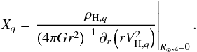 (A.1)where VH,q is the circular velocity produced by an oblate halo ρH,q. (Detailed formulae can be found e.g. in Banerjee et al. 2009.) Clearly Xq reduces to 1 for a spherical halo q = 1, for which the spherical Gauss law can be used. In Fig. A.1 we have plotted Xq as a function of q. As one can see the effect is rather weak, of the order of 5%, given a limited oblateness of 0.9−1, near the upper end.
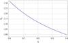 |
Fig. A.1 Effect of the DM halo oblateness q. |
It is worth stressing that even a halo oblateness outside this reference range can be straightforwardly taken into account by the quantity Xq. This is another advantage of the proposed method with respect to the traditional one. It is in fact much easier to introduce a constant factor of order one in Eq. (7), than to consider the effect of the halo oblateness in fitting a global mass model, where it triggers an additional non-uniqueness in the structural parameters.
Appendix B: Effect of finite disk thickness
For the sake of completeness here we also discuss the effect of the finite disk thickness. By neglecting it one would slightly overestimate the acceleration produced by a given disk mass. This can be noted from Fig. B.1, where we plot a correction factor for the “disk” part appearing on the rhs of Eq. (7):
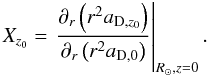 As one can see, given that the disk thickness is measured fairly well, z0 = 0.240−0.250 kpc (Jurić et al. 2008) the effect is very weak, of the order of 5% (with an uncertainty < 1%). Since this is much less than the uncertainty on the disk mass, we neglected it in the text, but it may be readily included in the ad term on the rhs of Eq. (7).
 |
Fig. B.1 Effect of the disk thickness z0. |
Appendix C: Issues in global approaches
The standard CO method reproduces by a maximum likelihood analysis a heterogeneous set of data (among them terminal and dispersion velocities, z-motions etc.) with an even more heterogeneous, large set of free parameters (among them R⊙, the disk and halo masses, the anisotropy in the motions of tracers of the gravitational field etc.), after which a number of crucial assumptions are taken. In this way it also obtains ρ⊙, as a byproduct. This strategy does not guarantee that the global MW model obtained is physically meaningful, even at the central best fit value of the parameters. For instance, the global model produces three independent and different estimates of V(r): 1) from the HI terminal velocities VT(r) (via V(r) = VT(r) + V⊙ r / R⊙); 2) from the halo stars dispersion velocities (via the Jeans equation); and 3) from the gravitational potential produced by the MW mass distribution. Clearly, by physical consistency, these three estimates of V(r) must agree, but in the strategy commonly employed there is nothing forcing this to happen.
In fact, let us look at the Galaxy global model obtained recently by this method by Catena & Ullio (2010). The above 3 different estimates of V(r) are obtained by using the best fit model parameters as given in their Tables 2 and 3. We find (Fig. C.1) that they disagree by 10% in amplitude and 0.3 in slope, quantities more than allowed by the observational errors. This implies that this method has an intrinsic uncertainty that may lead to a biased measure of ρ⊙ and of its uncertainty.
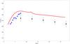 |
Fig. C.1 Different estimates of the circular velocity of the Milky Way, resulting from the global mass model of Catena & Ullio (2010). These are obtained from the gravitational potential (solid line), the HI terminal velocities (Malhotra 1995) (blue points), and velocity dispersions (Xue et al. 2008) (black points). |
All Figures
|
Fig. A.1 Effect of the DM halo oblateness q. |
| In the text | |
|
Fig. B.1 Effect of the disk thickness z0. |
| In the text | |
|
Fig. C.1 Different estimates of the circular velocity of the Milky Way, resulting from the global mass model of Catena & Ullio (2010). These are obtained from the gravitational potential (solid line), the HI terminal velocities (Malhotra 1995) (blue points), and velocity dispersions (Xue et al. 2008) (black points). |
| In the text | |
Current usage metrics show cumulative count of Article Views (full-text article views including HTML views, PDF and ePub downloads, according to the available data) and Abstracts Views on Vision4Press platform.
Data correspond to usage on the plateform after 2015. The current usage metrics is available 48-96 hours after online publication and is updated daily on week days.
Initial download of the metrics may take a while.