| Issue |
A&A
Volume 523, November-December 2010
|
|
|---|---|---|
| Article Number | A68 | |
| Number of page(s) | 6 | |
| Section | Cosmology (including clusters of galaxies) | |
| DOI | https://doi.org/10.1051/0004-6361/201014360 | |
| Published online | 18 November 2010 | |
Gravitational fluctuations of the galaxy distribution
1
Enrico Fermi Center, Piazza del Viminale 1, 00184
Rome,
Italy
2
Istituto dei Sistemi
Complessi CNR, via dei Taurini
19, 00185
Rome, Italy
e-mail: This email address is being protected from spambots. You need JavaScript enabled to view it.
Received:
5
March
2010
Accepted:
12
July
2010
Abstract
Aims. We study the statistical properties of the gravitational field generated by galaxy distribution observed by the Sloan Digital Sky Survey (DR7). We characterize the probability density function (PDF) of gravitational force fluctuations and relate its limiting behaviors to the correlation properties of the underlying density field. In addition, we study whether the PDF converges to an asymptotic shape within sample volumes.
Methods. We consider several volume-limited samples of the Sloan Digital Sky Survey and we compute the gravitational force probability density function (PDF). The gravitational force is computed in spheres of varying radius as is its PDF.
Results. We find that (i) the PDF of the force displays features that can be understood in terms of galaxy two-point correlations and (ii) density fluctuations on the largest scales probed, i.e. r ≈ 100 Mpc h-1, still contribute significantly to the amplitude of the gravitational force.
Conclusions. Our main conclusion is that fluctuations in the gravitational force field generated by galaxy structures are also relevant on scales ~100 Mpc h-1. By assuming that the gravitational fluctuations in the galaxy distribution reflect those in the whole matter distribution, and that peculiar velocities and accelerations are simply correlated, we may conclude that large-scale fluctuations in the galaxy density field may be the source of the large-scale flows recently observed.
Key words: cosmology: observations / large-scale structure of Universe
© ESO, 2010
1. Introduction
One of the main problems in studying the dynamics of a system of point masses concerns the analysis of the force acting on a test particle. This analysis can be achieved by determining of the statistical properties of the (Newtonian) gravitational field generated by the given point-mass distribution. From this study in general one can derive several useful pieces of information about the statistical and dynamical properties of the given point-mass distribution (Chandrasekhar 1943; Antonuccio-Delogu & Atrio-Barandela 1992; Gabrielli et al. 19991, 2004; Gabrielli 2005; Gabrielli et al. 2006, 2005). It has been known since the pioneering article of Chandrasekhar (1943) that, when particles are distributed without correlations (i.e., a Poisson distribution), the second moment of the gravitational force diverges. Certain spatial correlations between particles may cause the divergence, for instance, of the first moment (Gabrielli et al. 19991). For this reason, instead of computing the moments of the gravitational force, it is more appropriate to determine its probability density function (PDF). In particular, to understand the relevant features of the gravitational force fluctuations, it is interesting to study the limiting behaviors of the PDF in both strong and weak fields. It can be shown (see below) that the former is closely related to the small scale two-point correlation properties of the distribution. On the other hand, the weak field behavior is determined, in a non-trivial way, by how rapidly the distribution becomes isotropic on large scales. Therefore, this latter behavior is connected to the higher order correlation properties of the distribution (Gabrielli et al. 19991, 2005, 2006).
Our first aim, in this paper, is to consider the determination of the PDF of the gravitational force generated by the observed spatial distribution of galaxies. Given that the galaxy distribution is described as a stochastic point process, the statistical properties of the gravitational field on an arbitrary point is itself a stochastic quantity. The properties of these two stochastic processes are closely related. In particular, the force PDF can be simply regarded as a particular statistical characterization of the galaxy distribution containing some useful statistical information about higher order galaxy correlations.
To connect the force PDF of the galaxies with that of the whole mass distribution, we have to make an hypothesis about the relation between luminous and dark matter. The most simple assumption is that the galaxies trace the peaks of the underlying matter density field, i.e., that the galaxy density field is linearly biased with respect to the dark matter density field. If this is so, then the fluctuations in the gravitational force in the galaxy distribution also reflect those in the full matter distribution.
This is actually the standard hypothesis that is usually assumed in studies that compare of the dipole induced by the gravitational influence of structures in our local Universe with the observed CMB dipole1. Nowadays, several groups have shown that structures responsible for the dipole must be located on scales larger than ~150 Mpc h-1 (Maller et al. 2003). However, because of the sparseness of data at very large distances and the incompleteness of galaxy surveys, there is still no consensus about the depth of the convergence for the CMB dipole (Lavaux et al. 2008).
The actual dipole caused by structures around us corresponds to a determination of the force around a single point of the galaxy distribution (our galaxy). On the other hand, the PDF is determined by computing the gravitational force on each galaxy contained in a given catalog, and by repeating this measurement for all measured galaxies. With respect to the single determination, the PDF has several advantages: (i) it considers complete samples extracted from galaxy redshift surveys (i.e., volume-limited samples) without making any additional assumption about the incompleteness of the catalogs; (ii) we do not have to consider the sky regions where observations were not done and use weighting schemes to correct for this incompleteness. We indeed compute the force only in spherical volumes fully contained in our samples; (iii) by considering each galaxy as a center, we determine the force generated by all galaxies contained in a spherical volume around it. We can therefore evaluate the statistical significance that the determination of the force from a single point (i.e., the dipole) is (or is not) found to converge to an asymptotic value within a certain distance.
It is then interesting to consider the relation between the gravitational force field g and the peculiar velocity field v. In the linear regime of low-amplitude density fluctuations, it is well-known that the velocity is proportional to the gravitational acceleration (Peebles 1980). As our observations are limited to a range of scales in which galaxy fluctuations are still large, we can only speculate about the relation between the gravitational force and the peculiar velocity fields by assuming that there is a direct proportionality even in the non-linear regime. In this respect we note that when fluctuations are large and the universe is curvature-dominated (i.e., with negligible matter content) one still finds that v ∝ g (Joyce et al. 2000). The relation between g and v has acquired interest because of the increasing number of observations of peculiar velocities on large scales.
Peculiar velocities provide important dynamical information because they are related to the large-scale matter distribution. By studying their local amplitudes and directions, these velocities allow us, in principle, to probe deeper, or hidden, parts of the Universe. The peculiar velocities are indeed directly sensitive to the total matter content, inferred from its gravitational effects, and not only to the luminous matter distribution. However, their direct observation by means of distance measurements remains a difficult task. There have been observations of large-scale galaxy coherent motions that are at odds with standard cosmological models. For instance, Watkins et al. (2009) measured in a Gaussian window of diameter 100 Mpc h-1, a coherent bulk motion of 407 ± 81 km s-1, which conflicts with the prediction of ≈ 200 km s-1 at the 2σ level of LCDM. Other independent results confirm the presence of unexpectedly large bulk motions (Lavaux et al. 2008; Kashlinsky et al. 2008, 2010). In particular, Kashlinsky et al. (2008) measured peculiar velocities of galaxy clusters by studying, in a large statistical sample of clusters, the fluctuations in the cosmic microwave background (CMB) generated by the kinematic Sunyaev-Zeldovich (KSZ) effect, i.e., caused by the scattering of microwave photons by the hot X-ray emitting gas inside clusters. They measured a bulk flow of 600–1000 km s-1 on scales > 300 Mpc h-1 (the limit of the considered clusters catalog) which is more than 10 times larger than expected by the LCDM model. In addition, they concluded that the coherence length of the measured bulk flow shows no signs of convergences out to the largest probed scales. Kashlinsky et al. (2010), by applying the KSZ method to a larger cluster sample, showed that the flow is consistent with approximately constant velocity out to at least ≃ 800 Mpc h-1. Although these results remain controversial (Keisler 2009), measurements of peculiar velocities have very interesting potentials and future surveys are expected to provide more precise data of bulk flow motion on large scales (Smith et al. 2004; Frieman et al. 2008). Our aim here is to verify whether, based on the assumption that v ∝ g, fluctuations in the force distribution should be compatible with the large-scale bulk flows observed. If this were so, this would indicate that local galaxy structures may represent an important contribution to the peculiar velocities that could avoid us having to invoke exotic physics, as the effect of far-away pre-inflationary inhomogeneities, to explain the large-scale bulk flows (Kashlinsky et al. 2008).
In this paper, we focus on the following two questions: (i) what is the shape of the force PDF and how is this connected to the underlying fluctuations in the galaxy density field? (ii) Is there a convergence of the PDF to an asymptotic shape that is independent of the size of the volume (i.e., the sphere radius r) in which this is computed. Based on the assumption that light traces mass, we are unable to determine the direction and amplitude of the dipole around us, thus verify whether this is the same as the CMB dipole. However, we can characterize the properties of gravitational fluctuations generated by galaxy structures in a complete statistical way (up to the maximum scale Rs allowed by the geometry of available samples); in particular, we can determine whether in the volumes considered the gravitational force has reached, from a statistical point of view, saturation on scales rf < Rs. In this case, fluctuations on scales larger than rf do not contribute anymore, statistically, to the amplitude of the gravitational force. That is, large-scale contributions to the force from different directions tend to compensate each other. The scale rf would thus be the scale beyond which large scale flows would start to decay in amplitude. On the other hand, if we were able to place only a lower limit on the scale rf, i.e. if rf > Rs without a convergence of PDF to a stable shape within the sample volume, this would corroborate the conjecture that large-scale flows can be sourced by fluctuations in the density field that statistically break spherical symmetry. In this case, larger and larger volumes would continue to contribute to the gravitational force on an average galaxy. Therefore, if the measurements of large-scale bulk flows are unaffected by major statistical and systematical effects, but are generated instead by galaxy density inhomogeneities, we would expect not to see a convergence of the PDF to a stable shape inside the considered samples because we are limited to a volume of radius Rs ≈ 100 Mpc h-1. As discussed above, while the information on the force PDF of galaxies can be derived in a straightforward way from the data, its relation to the peculiar velocity field is based on a series of assumptions. Nevertheless, it is interesting to consider whether when galaxies trace mass and peculiar velocities are parallel to accelerations, it is possible to learn something about the relation between the force and peculiar velocity fields.
The paper is organized as follows. In Sect. 2, we briefly review some basic properties of the gravitational force field in stochastic point distributions. We then describe the selection of the galaxy samples in Sect. 3 and the methods (Sect. 4) used to estimate the relevant statistical quantities in the data. In Sect. 5, we discuss our main results and in Sect. 6 we consider the PDF of the gravitational force in mock galaxy catalogs generated from cosmological N-body simulations. We finally draw our main conclusions in Sect. 7.
2. Gravitational force from stochastic point distributions
The value of the gravitational force acting on a particle belonging to a given point distribution is determined by both the immediate neighborhood of the particle itself and the large-scale properties of the system. This situation reflects two peculiar features of the gravitational force, that it is divergent at small separations and is slowly, i.e., in accordance with a power-law, decaying at large distances. The stochastic nature of a given point distribution generates a certain PDF P(F) of the gravitational force F. In general, one would like to calculate P(F) from the statistical properties of the underlying particle distribution. There are a few examples of particle distributions with analytically calculable P(F). Chandrasekhar (1943) was the first to compute the PDF of the gravitational force for an uncorrelated distribution of points, i.e. the Poisson distribution. In this situation, the PDF of the force is found to be given exactly by the Holtzmark distribution (HD), which is a three-dimensional fat (or heavy) tailed Lévy distribution. Approximated generalizations of this approach can be found for more complex particle systems obtained by perturbing a Poisson distribution (Gabrielli et al. 2004) or perturbing a perfect cubic lattice of particles (Gabrielli et al. 2006). Vald (1994) developed a functional integral approach for evaluating the stochastic properties of vectorial additive random fields generated by a variable number of point sources obeying inhomogeneous Poisson statistics. In this way he derived the generalized Holtzmark distribution (GHD), which we discuss in more detail below.
The gravitational force for unit mass due to the N particles contained in a sphere C(r,xi) of radius r centered on the ith particle of a given distribution is  (1)where G is the gravitational constant, mj is the jth particle mass, and N is the number of particles in a given volume V. In what follows, we take G = 1 and we consider particles with the same mass, so that we assume that mi = 1∀i.
If the particle distribution is statistically stationary, i.e. it is invariant under space rotations and translations, the direction of F has equal probability in each direction, i.e. P(F) depends only on the force modulus F = | F | . For this reason, we can consider the PDF W(F) of the force modulus F, which is simply related to the three dimensional PDF by W(F) = 4πF2P(F).
The statistical properties of a density field can be characterized by measuring the average conditional density defined as (Sylos Labini et al. 2009a)  (2)where ni(r) is the density measured in a sphere of radius r centered on the ith particle, and the second equality holds only for the case in which there are power-law correlations in a certain range of scales. In Eq. (2), the constant A is related to the average nearest neighbor (NN) distance Λ ≈ A − 1 / D and γ = 3 − D is the correlation exponent2. When there are power-law correlations on small scales one can readily derive an expression for the force PDF due only to a NN particle by using the identity (Gabrielli et al. 2005)
  (3)where
  (4)is the NN PDF for a particle system obeying to Eq. (2)3. For D = 3, Eq. (4) reduces to the well-known expression for the Poisson NN PDF (Chandrasekhar 1943). Thus, from Eqs. (3, 4) we can derive the NN force PDF
 ![Mathematical equation: \begin{equation} \label{eqWnnD1} W_{nn}(F;D) = \frac{D}{2} F_\Lambda^{D/2} F^{-\frac{D+2}{2}} \exp\left[ - \left(\frac{F_\Lambda}{F}\right)^{D/2} \right], \end{equation}](/articles/aa/full_html/2010/15/aa14360-10/aa14360-10-eq43.png) (5)where
(5)where  For D = 3, Eq. (5) reduces to the Poisson case (Chandrasekhar 1943). The asymptotic behavior in the strong field limit is
  (6)It is simple to show that the average force diverges for D > 2 and that the average square force diverges ∀D ≤ 3. For this reason, as mentioned in the introduction, we do not directly consider the study of these moments, while we focus on the shape of the PDF.
Vald (1994) derived a simple expression for the GHD, which holds when there are only power-law two-point correlations as in Eq. (2) and no higher order ones (see also the discussion in Gabrielli et al. 19991). The GHD can be written as  (7)where β = F / F0,
  (8)the constant F0 is given by
  (9)and the symbol ΓE represents the Euler Gamma function. For D = 3, Eqs. (7–9) reduces to the HD. It is easy to show that in the strong field limit W(F;D) → Wnn(F;D), so that the fat tail is always present and due to NN correlations.
The PDF of the vector F, i.e. P(F), must be symmetrical about zero, because the distribution is isotropic and the average of the vector force must be zero. Thus P(0) = const., so that we have 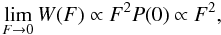 (10)which is indeed the case for both the HD and the GHD. Hence the limiting behaviors of the GHD (and of the HD for D = 3) are
 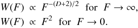 (11)The strong field limit is determined by the small-scale correlation properties, while the weak field limit is very general and related to the stationarity of the distribution. We focus on these tails in the analysis of the galaxy samples.
We emphasize that Eq. (2) may describe an highly inhomogeneous structure characterized by large fluctuations and non-trivial higher order correlations (Gabrielli et al. 2005). In this a situation neglecting higher order correlations is a very crude approximation. However, only in this limit is one able to calculate the force PDF. By taking into account higher order correlations, one may compute only few moments of the force (Gabrielli et al. 19991, 2005). This means that, while the limiting behaviors given by Eq. (11) are expected to be satisfied as long as Eq. (2) holds and the particle distribution is stationary, the exact location of the peak, marking the transition from W(F) ∝ F − (D + 2) / 2 to W(F) ∝ F2, is poorly constrained from a theoretical point of view.
We note that Eq. (2) may also describe a structure that has varying correlations as a function of scale. In this case, D = D(r) ≤ 3 where D = 3 when the distribution becomes spatially uniform and the average conditional density coincides with the unconditional density, modulo small-amplitude correlations described by the reduced correlation function ξ(r) (Gabrielli et al. 2005). Only in this situation may one describe the properties of the force PDF in terms of either the ξ(r) function or its Fourier transform, the power spectrum (Gabrielli et al. 2004, 2006, 2005; Joyce 2007).
3. The data
We extracted a volume-limited (VL) sample constructed from the data release 7 (DR7) (Abazajian et al. 2009) of the SDSS (see Sylos Labini et al. 2009a; Antal et al. 2009, for details). To compute the metric distance, we used the standard cosmological parameters ΩM = 0.3 and ΩΛ = 0.7. We considered a contiguous sky area with almost uniform coverage and we applied K-corrections to calculate absolute magnitude Mr in the r band (corrected for Galactic absorption) as in Sylos Labini et al. (2009a).
Main properties of the obtained VL samples with K-corrections and without E-corrections.
We selected three samples (see Table 1). The sample VL1, containing about one fifth of all galaxies in DR7, has relatively large spatial extensions and small spread in galaxy luminosity. On the other hand, the sample VL2 contains fainter galaxies and covers a smaller volume, while VL3 contains brighter galaxies and is more extended in radial distance.
In Table 1 we also report the average distance between nearest neighboring galaxies: this provides a lower cut-off for the computation of real-space statistical properties. It is also directly related to the large-field tail of the PDF of the force. The fainter the galaxies, clearly, the smaller the value of Λ (Gabrielli et al. 2005).
We do not apply any correction for redshift distortion,thus our results are given in redshift space. We expect the peculiar velocities to affect the small-scale properties, where their redshift distortions are relatively important, of the statistical quantities we measured but to leave conclusions on large scales unchanged.
4. Methods
The average conditional density in Eq. (2) is computed by evaluating, on the scale r, the average of the N(r) density determinations over the sample points whose minimal distance from sample boundaries is smaller than r. The force F (Eq. (1)) is computed in a sphere of radius r centered on a galaxy with the same constraint as above, so that only complete spheres are considered. This implies that the number of determinations depends on the scale r (Sylos Labini et al. 2009a). We limit the analysis to N(r) ≥ 104. We note that the force PDF we compute here is intrinsically defined for a discrete and stochastic point distribution. As long as these points (galaxies) display non-trivial spatial correlations, the force PDF deviates from the Holtzmark distribution.
5. Results
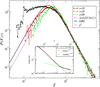 |
Fig. 1 PDF of the force for the VL1 computed one different scales r. The solid line is Eq. (7) with the parameters from Eq. (12). In the inset panel, the behavior of the average conditional density is plotted in addition to its best fits for r < 20 Mpc h-1 and for 20 < r < 80 Mpc h-1. |
We find that the average conditional density for the VL1 sample (see Fig. 1, inset panel) behaves for r < 20 Mpc h-1 as 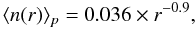 (12)while for 20 < r < 80 Mpc h-1 we get ⟨ n(r) ⟩ p = 0.0058 × r-0.26 (Antal et al. 2009)4. This behavior implies that a crossover toward homogeneity not being found up to ~80 Mpc h-1. This implies that fluctuations are still large when filtered on scales ~80 Mpc h-1 and that the standard two-point correlation function ξ(r) results, which are biased by major systematic effects in these samples, may underestimate the amplitude of fluctuations on scales > 10 Mpc h-1 (see the discussion in Sylos Labini et al. 2009a,d).
In other two samples considered, VL2 and VL3, we found similar behaviors (see Figs. 2, 3): (i) the PDF of the force does not converge to an asymptotic shape up to ~100 Mpc h-1 and (ii) the conditional density correspondingly does not exhibit a well defined trend toward homogenization.
In Fig. 1, the PDF of the force for the SDSS-VL1 is shown at different scales r. We note that the large field tail is stable for all sphere radii considered. It is characterized by a power-law behavior of the type W(F) ~ F − α with α = −2.1. From Eq. (5), we infer that D = 2.2, thus in agreement with the value found for the conditional density on small scales (i.e., Eq. (12)). Thus the validity of the approximation at large F values can be simply explained by very small-scale considerations. For r = 30 Mpc h-1, the GHD obtained from Eqs. (7–9) with the values of A,D measured from the best fit of the conditional density for r < 20 Mpc h-1, fits the data extremely well. (i.e. Eq. (12)). In this case, there are no free parameters to be adjusted. In addition, we note that the weak force tail is proportional to F2, in agreement with Eq. (11).
For r = 90 Mpc h-1, the same fit with the GHD, for small F values, is not as good as for the previous case, while it behaves again as F2 in agreement with Eq. (11). This is because the contribution to the gravitational field from the largest scales in this sample are non-negligible, and in addition the average conditional density displays a different slope for r > 20 Mpc h-1 than for r < 20 Mpc h-1. This implies that the GHD distribution is only an approximation to the real PDF. It is indeed clear that the simplifying assumptions used to derive Eqs. (7–9), and in particular the hypothesis that there are no n-point correlations, are too naive with respect to the complexity of the true galaxy structure. The value of the field at which the turnover of the PDF occurs, depends on the sphere radius r determining the cut-off to the force calculation in the data. This implies that up to the largest sphere radius considered we do not find a convergence of the force PDF to an asymptotic behavior. The PDF peak instead shifts toward stronger field values at larger r, implying that greater and greater contributions are given by the large scale fluctuations. We note that there is a factor of three between the PDF peak location at r = 10 Mpc h-1 and at r = 90 Mpc h-1 while the peak of the PDF increases by 20% from r = 50 Mpc h-1 to r = 90 Mpc h-1. It is surely smaller than from r = 10 Mpc h-1 to r = 50 Mpc h-1 but this implies that a non-negligible contribution to the force field is caused by large-scale fluctuations.
6. Comparison with mock galaxy catalogs
To compare the results obtained in the data with the theoretical predictions, we considered a semi-analytic galaxy catalog constructed from the Millennium LCDM N-body simulation (Springel et al. 2005). To construct mock samples corresponding to SDSS VL samples, we used the full version of the catalog in the ugriz filter system. The catalog contains about 9 million galaxies in a 500 Mpc h-1 cube (Croton et al. 2006)5. We use the absolute magnitudes in r filter used in the SDSS case, to construct the mock samples with the same limits in absolute magnitude as for the SDSS VL samples with K-corrections. As for the real data, we considered the redshift-space distribution (more details on the construction of mock samples can be found in Sylos Labini et al. 2009a). The average distance between the nearest points in the mock galaxy sample for which we present results is Λ ~ 1.6 Mpc h-1, i.e. about that of the sample VL1 of SDSS. We note however that in other mock samples we found very similar results to the ones discussed here.
The main features of the considered statistics in the mock galaxy samples are (see Fig. 4) (i) beyond a few tens of Mpc the PDF stabilizes to an asymptotic (sample-independent) shape and (ii) the conditional density exhibit a well-defined flattening on large enough scales. Both these behaviors differ from those found in the real data.
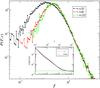 |
Fig. 4 PDF of the force for the mock sample computed on different scales r. In the inset panel, we plot the behavior of the average conditional density. |
To conclude this section, we note that in LCDM models, on large enough scales, one expects the force PDF to be sample-size independent. In general, if the variance of the force is finite, the force PDF is necessarily well defined. From the definition of the force, and after transforming into Fourier space we find that (Joyce 2007)
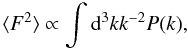 where P(k) is the power spectrum of the density field. Therefore, a sufficient condition for the force to be defined in the usual thermodynamic limit is just that k-2P(k) be integrable (Joyce 2007). Since we are interested here in only the possible divergences in this quantity caused by the long distance behavior of the fluctuations, it is therefore sufficient that we assume that limk → 0kP(k) = 0. Thus it follows that the force is well defined in the infinite volume limit if P(k) diverges more slowly at small k than k-1. This condition is satisfied by standard cosmological density fields for which P(k) ~ k on large enough scales, i.e. r > 100 Mpc h-1 (Sylos Labini and Vasilyev 2008).
7. Conclusions
The gravitational force probability density (PDF) in finite volumes represents an interesting characterization of the statistical properties of a given point distribution which is directly related to the statistical properties of density fluctuations and their dynamical effects on large scales. By analyzing only the statistical properties of the force PDF we have found that this PDF is in general related to two-point and higher order correlations. We have measured the PDF in several galaxy samples of the SDSS finding that (i) its limiting behaviors can be simply inferred from the galaxy correlation properties and that (ii) the PDF does not achieve an asymptotic, sample-size-independent, shape within the volumes considered, i.e. ~100 Mpc h-1. These results agree with the studies of the local dipole due to structures, and in particular those that do not find a convergence up to ~100 Mpc h-1.
The relation between the force PDF and the dynamics, i.e. between gravitational acceleration and peculiar velocity fields requires several comments. First, we have to assume that galaxies trace the underlying matter density field, at least on large enough scales (i.e., that biasing is linear). This is a reasonable assumption usually employed in the studies of the dipole due to structures (Maller et al. 2003; Lavaux et al. 2008). It is then necessary to assume that peculiar velocities are parallel to gravitational accelerations. This can be verified by linear perturbation theory (Peebles 1980) or when fluctuations are large but the universe is in a curvature-dominated phase (Joyce et al. 2000). By using these assumptions, we conclude that the observed
values of the bulk flows are compatible with the gravitational force fluctuation field from galaxy structures.
In other words, these results support the conjecture that large-scale structures may be the source of the observed large-scale flows, which are unexpected in the standard LCDM scenario. We note that even the correlation properties of the galaxy density field in the SDSS samples are also at odds with the standard LCDM predictions (Sylos Labini et al. 2009a,b,c,d,e).
The results of this paper corroborate that the observed large-scale flows are due to large-scale fluctuations in the galaxy density field. A more quantitative conclusion must consider the dynamical history of structure formation and is beyond the scope of this paper.
This shows that our Local Group moves with a velocity of 627 ± 22 km s-1 towards the direction l = 276° and b = 306° in Galactic coordinates.
Note that D is not the space dimension, but it can be interpreted as the fractal dimension of the object (Gabrielli et al. 2005).
More precisely, Eq. (4) is found when higher order correlations are neglected.
The relation between the conditional density and the standard two-point correlation function, and in particular the relation between their respective exponents in a finite sample is discussed in Gabrielli et al. (2005, see pp. 240–242).
See http://www.mpa-garching.mpg.de/galform/agnpaper/ for semi-analytic galaxy data files and description, and see http://www.mpa-garching.mpg.de/millennium/ for information on Millennium LCDM N-body simulation.
Acknowledgments
I am grateful to Yuri V. Baryshev, Andrea Gabrielli, Michael Joyce and Nickolay L. Vasilyev for useful discussions and collaborations. I acknowledge the use of the Sloan Digital Sky Survey data (http://www.sdss.org), of the NYU Value-Added Galaxy Catalog (http://ssds.physics.nyu.edu/) and of the Millennium run semi-analytic galaxy catalog (http://www.mpa-garching.mpg.de/galform/agnpaper/).
References
- Abazajian, K. N., Adelman-McCarthy, J. K., Agüeros, M. A., et al. 2009, ApJS, 182, 543 [NASA ADS] [CrossRef] [Google Scholar]
- Antal, T., Sylos Labini, F., Vasilyev, N. L., & Baryshev, Yu. V. 2009, Europhys. Lett., 88, 59001 [NASA ADS] [CrossRef] [Google Scholar]
- Antonuccio-Delogu, V., & Atrio-Barandela, F. 1992, ApJ, 392, 403 [NASA ADS] [CrossRef] [Google Scholar]
- Chandrasekhar, A. 1943, Rev. Mod. Phys., 15, 1 [NASA ADS] [CrossRef] [Google Scholar]
- Croton, D. J., Springel, V., White, S. D. M., et al. 2006, MNRAS, 365, 11 [NASA ADS] [CrossRef] [Google Scholar]
- Gabrielli, A. 2005, Phys. Rev. E, 72, 066113 [NASA ADS] [CrossRef] [Google Scholar]
- Gabrielli, A., Sylos Labini, F., & Pellegrini, S. 1999, Europhys. Lett., 46, 127 [NASA ADS] [CrossRef] [Google Scholar]
- Gabrielli, A., Masucci, P. A., & Sylos Labini, F. 2004, Phys. Rev. E, 69, 031110 [NASA ADS] [CrossRef] [Google Scholar]
- Gabrielli, A., Sylos Labini, F., Joyce, M., & Pietronero L. 2005, Statistical Physics for Cosmic Structures (Berlin: Springer Verlag) [Google Scholar]
- Gabrielli, A., Joyce, M., Marcos, B., Sylos Labini, F., & Baertschiger, T. 2006, Phys. Rev. E, 74, 021110 [NASA ADS] [CrossRef] [MathSciNet] [Google Scholar]
- Frieman, J. A., et al. 2008, A&A, 479, 9 [Google Scholar]
- Kashlinsky, A., Atrio-Barandela, F., Kocevski, D., & Ebeling, H. 2008, ApJ, 686, L49 [NASA ADS] [CrossRef] [Google Scholar]
- Kashlinsky, A., Atrio-Barandela, F., Ebeling, H., Edge, A., & Kocevski, D. 2010, ApJ, 712, L81 [NASA ADS] [CrossRef] [Google Scholar]
- Keisler, R. 2009, ApJ, 707, L42 [NASA ADS] [CrossRef] [Google Scholar]
- Joyce, M. 2008, AIP Conf. proc., 970, 237 [NASA ADS] [CrossRef] [Google Scholar]
- Joyce, M., Anderson, P. W., Montuori, M., Pietronero, L., & Sylos Labini, F. 2000, Europhys. Lett., 50, 416 [NASA ADS] [CrossRef] [EDP Sciences] [Google Scholar]
- Lavaux, G., Tully, R. B., Mohayaee, R., & Colombi, S. 2010, ApJ, 709, 483 [NASA ADS] [CrossRef] [Google Scholar]
- Maller, A. H., McIntosh, D. H., Katz, N., & Weinberg, M. D. 2003, ApJ, 598, L1 [NASA ADS] [CrossRef] [Google Scholar]
- Peebles, P. J. E. 1980, Large Scale Structure of the Universe (Princeton, New Jersey: Princeton University Press) [Google Scholar]
- Smith, R. J., Hudson, M. J., Nelan, J. E., et al. 2004, AJ, 128, 1558 [NASA ADS] [CrossRef] [Google Scholar]
- Springel, V., White, S. D. M., Jenkins, A., et al. 2005, Nature, 435, 629 [NASA ADS] [CrossRef] [PubMed] [Google Scholar]
- Sylos Labini, F., & Vasilyev, N. L. 2008, A&A, 477, 381 [NASA ADS] [CrossRef] [EDP Sciences] [Google Scholar]
- Sylos Labini, F., Vasilyev, N. L., & Baryshev, Y. V. 2009a, A&A, 508, 17 [NASA ADS] [CrossRef] [EDP Sciences] [Google Scholar]
- Sylos Labini, F., Vasilyev, N. L., Pietronero, L., & Baryshev, Y. V. 2009b, Europhys. Lett., 86, 49001 [NASA ADS] [CrossRef] [Google Scholar]
- Sylos Labini, F., Vasilyev, N. L., & Baryshev, Y. V. 2009c, Europhys. Lett., 85, 29002 [NASA ADS] [CrossRef] [EDP Sciences] [Google Scholar]
- Sylos Labini, F., Vasilyev, N. L., & Baryshev, Y. V. 2009d, A&A, 496, 7 [NASA ADS] [CrossRef] [EDP Sciences] [Google Scholar]
- Sylos Labini, F., Vasilyev, N. L., Baryshev, Y. V., & López-Corredoira, M. 2009e, A&A, 505, 981 [NASA ADS] [CrossRef] [EDP Sciences] [Google Scholar]
- Vlad, M. O. 1994, Astrophys. Space. Sci., 218, 159 [NASA ADS] [CrossRef] [Google Scholar]
- Watkins, R., Feldman, H. A., & Hudson, M. J. 2009, MNRAS, 392, 743 [NASA ADS] [CrossRef] [Google Scholar]
All Tables
Main properties of the obtained VL samples with K-corrections and without E-corrections.
All Figures
|
Fig. 1 PDF of the force for the VL1 computed one different scales r. The solid line is Eq. (7) with the parameters from Eq. (12). In the inset panel, the behavior of the average conditional density is plotted in addition to its best fits for r < 20 Mpc h-1 and for 20 < r < 80 Mpc h-1. |
| In the text | |
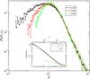 |
Fig. 2 The same of Fig. 1 but for the sample VL2. |
| In the text | |
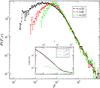 |
Fig. 3 The same of Fig. 1 but for the sample VL3. |
| In the text | |
|
Fig. 4 PDF of the force for the mock sample computed on different scales r. In the inset panel, we plot the behavior of the average conditional density. |
| In the text | |
Current usage metrics show cumulative count of Article Views (full-text article views including HTML views, PDF and ePub downloads, according to the available data) and Abstracts Views on Vision4Press platform.
Data correspond to usage on the plateform after 2015. The current usage metrics is available 48-96 hours after online publication and is updated daily on week days.
Initial download of the metrics may take a while.