| Issue |
A&A
Volume 522, November 2010
|
|
|---|---|---|
| Article Number | A41 | |
| Number of page(s) | 6 | |
| Section | The Sun | |
| DOI | https://doi.org/10.1051/0004-6361/201015167 | |
| Published online | 29 October 2010 | |
Spectral line polarization with angle-dependent partial frequency redistribution
I. A Stokes parameters decomposition for Rayleigh scattering
UNS, CNRS, OCA, Laboratoire Cassiopée,
BP 4229,
06304
Nice Cedex 4,
France
e-mail: This email address is being protected from spambots. You need JavaScript enabled to view it.
Received:
7
June
2010
Accepted:
30
July
2010
Abstract
Context. The linear polarization of a strong resonance lines observed near the solar limb is created by a multiple-scattering process. Partial frequency redistribution (PRD) effects must be accounted for to explain the polarization profiles. The redistribution matrix describing the scattering process is a sum of terms, each containing a PRD function multiplied by a Rayleigh type phase matrix. A standard approximation made in calculating the polarization is to average the PRD functions over all the scattering angles, because the numerical work needed to take the angle-dependence of the PRD functions into account is large and not always needed for reasonable evaluations of the polarization.
Aims. This paper describes a Stokes parameters decomposition method, that is applicable in plane-parallel cylindrically symmetrical media, which aims at simplifying the numerical work needed to overcome the angle-average approximation.
Methods. The decomposition method relies on an azimuthal Fourier
expansion of the PRD functions associated to a decomposition of the phase matrices in
terms of the Landi Degl’Innocenti irreducible spherical tensors for polarimetry
 (i Stokes parameter index,
Ω ray direction). The terms that depend on the azimuth of the
scattering angle are retained in the phase matrices.
(i Stokes parameter index,
Ω ray direction). The terms that depend on the azimuth of the
scattering angle are retained in the phase matrices.
Results. It is shown that the Stokes parameters I and
Q, which have the same cylindrical symmetry as the medium, can be
expressed in terms of four cylindrically symmetrical components  (K = Q = 0, K = 2,
Q = 0,1,2). The components with
Q = 1,2 are created by the angular dependence of the
PRD functions. They go to zero at disk center, ensuring that Stokes Q
also goes to zero. Each component is a
solution to a standard radiative transfer equation. The source term
(K = Q = 0, K = 2,
Q = 0,1,2). The components with
Q = 1,2 are created by the angular dependence of the
PRD functions. They go to zero at disk center, ensuring that Stokes Q
also goes to zero. Each component is a
solution to a standard radiative transfer equation. The source term
 are
significantly simpler than the source terms corresponding to I and
Q. They satisfy a set of integral equations that can be solved by an
accelerated lambda iteration (ALI) method.
are
significantly simpler than the source terms corresponding to I and
Q. They satisfy a set of integral equations that can be solved by an
accelerated lambda iteration (ALI) method.
Key words: line: formation / polarization / radiative transfer
© ESO, 2010
1. Introduction
The solar spectrum shows some strong resonance lines such as Ca ii H and K, Mg ii h and k, and Ca i 4227 Å . They are formed in the upper layers of the photosphere and lower chromosphere. The main mechanism presiding over their formation is radiative excitation of the lower level of the transition followed by spontaneous radiative deexcitation of the upper level. One of the difficulties that appears when investigating these lines is that the frequencies of the incoming and scattered beams are partially correlated, a phenomenon known as partial frequency redistribution (PRD). It is quite conspicuous in the wings of the intensity profiles and in the linear polarization profiles. Created by the scattering of the photospheric radiation, this linear polarization is known as resonance polarization or Rayleigh scattering in the classical physics description (Chandrasekhar 1950). It is at a maximum in the uppermost layers of the solar atmosphere where the anisotropy of the radiation field takes its highest values. It is thus mainly observed near the solar limb. Since Ivanov (1991) coined the term, it has often been referred to as the second solar spectrum. A high spectral resolution atlas of the second solar spectrum from 3160 Å to 6995 Å has been recorded by Gandorfer (2000, 2002, 2005).
Some spectral lines like Ca I 4227 Å can be modeled, at least for the purposes of polarization, by a two-level atom with unpolarized ground level. Each scattering event is characterized by a redistribution matrix that describes the coupling between frequencies, directions, and polarization of the incoming and scattered beams. The redistribution matrix proposed in Bommier (1997a) is the last and the most sophisticated of the expressions established to describe resonance polarization with partial frequency redistribution (PRD) effects. Starting from the non-LTE semi-classical theory of Stenflo (1976), continuous progress has been made in the direction of a better description of the PRD mechanism and of the role of elastic collisions. This was made possible by the use of the density matrix approach of Omont et al. (1972), which leads to a fully quantum mechanical description of the polarized radiation field and atomic structure. In the absence of a magnetic field, as shown by Bommier (1997a) (see also Domke & Hubeny 1988), the redistribution matrix is a sum of terms, each the product of a scalar redistribution function r(ν,ν′,Θ) by a polarization matrix P(Ω,Ω′) (see Eq. (20)). Here ν′ and ν are the frequencies of the incoming and scattered beams and Θ the scattering angle between the directions Ω′ and Ω of the beams (see Fig. 1). The scalar redistribution functions are of the rII or rIII type (Hummer 1962). They describe frequency coherent and frequency incoherent scattering in the atomic frame, respectively. Frequency coherent scattering plays an important role in the line wings. The dependence on the scattering angle appearing in the laboratory frame redistribution functions comes from the Doppler shifts created by the thermal velocities of the atoms. Since 1997, great progress has been made to properly include the Hanle and Zeeman effects (see e.g. Bommier 1997b; Sampoorna et al. 2007). Systematic theories for multi-level atoms incorporating PRD effects are still under development.
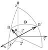 |
Fig. 1 Atmospheric reference system. The directions Ω and Ω′ are defined by their polar angles (θ,χ) and (θ′,χ′) and Θ is the scattering angle. The Z-axis is along the outside normal to the atmosphere. |
One of the difficulties with PRD from a numerical point of view is that the dependence on
the directions Ω and Ω′ appears
in the polarization matrices and in the scalar redistribution functions. For this reason the
angle-dependent redistribution functions
rII,III(ν,ν′,Θ)
are often replaced by their angle-averaged version  , with the averaging over
all the scattering angles. The expression proposed by Rees
& Saliba (1982) and the angle-averaged versions of Domke & Hubeny (1988) and Bommier
(1997a) have been used quite extensively, on the whole rather successfully (see e.g
Faurobert-Scholl 1996). For intensity profiles, this
approximation, which is based on the isotropy of the radiation field inside the atmosphere,
is indeed quite reasonable. It is definitely more questionable when one is interested in the
linear polarization that is directly controlled by the anisotropy of the intensity field. A
correct evaluation of the linear polarization is very important because it is a starting
point for quantitative determinations of micro-turbulent magnetic fields in the solar
atmosphere by the Hanle effect (e.g. Stenflo 1982;
Faurobert-Scholl 1996; Trujillo Bueno et al. 2004). Comparisons between
Q/I profiles calculated with
angle-dependent and angle-averaged PRD can be found in Faurobert (1987, 1988) and in Nagendra et al. (2002). For strong lines (total optical
thickness at line center around 104) differences shown in Faurobert (1988) for the ratio
Q / I appear to be large enough to be
measurable, but in Nagendra et al. (2002) they are
essentially negligible. These two articles use a rather different numerical approach. In
Faurobert (1988) it is tailored for Rayleigh
scattering, and in Nagendra et al. (2002) for the
Hanle effect.
, with the averaging over
all the scattering angles. The expression proposed by Rees
& Saliba (1982) and the angle-averaged versions of Domke & Hubeny (1988) and Bommier
(1997a) have been used quite extensively, on the whole rather successfully (see e.g
Faurobert-Scholl 1996). For intensity profiles, this
approximation, which is based on the isotropy of the radiation field inside the atmosphere,
is indeed quite reasonable. It is definitely more questionable when one is interested in the
linear polarization that is directly controlled by the anisotropy of the intensity field. A
correct evaluation of the linear polarization is very important because it is a starting
point for quantitative determinations of micro-turbulent magnetic fields in the solar
atmosphere by the Hanle effect (e.g. Stenflo 1982;
Faurobert-Scholl 1996; Trujillo Bueno et al. 2004). Comparisons between
Q/I profiles calculated with
angle-dependent and angle-averaged PRD can be found in Faurobert (1987, 1988) and in Nagendra et al. (2002). For strong lines (total optical
thickness at line center around 104) differences shown in Faurobert (1988) for the ratio
Q / I appear to be large enough to be
measurable, but in Nagendra et al. (2002) they are
essentially negligible. These two articles use a rather different numerical approach. In
Faurobert (1988) it is tailored for Rayleigh
scattering, and in Nagendra et al. (2002) for the
Hanle effect.
In this paper we describe a new method for calculating of the linear polarization when the
angle-dependence of the PRD is retained. The method is developed for a plane-parallel
atmosphere. It makes use of an azimuthal Fourier decomposition of the PRD functions and of
the decomposition of the elements of the polarization phase matrix in terms of the spherical
tensors for polarimetry  introduced by Landi Degl’Innocenti (1984) (see also Landi
Degl’Innocenti & Landolfi 2004, henceforth LL04). Here i
is a Stokes parameter index
(i = 0,...,3), and
K and Q are integer numbers
(K = 0,1,2 and
− K ≤ Q ≤ +K for each value of
K). The approach is somewhat similar to a method used in Frisch (2007, henceforth HF07) and Frisch (2009, henceforth HF09) for the weak-field Hanle effect.
introduced by Landi Degl’Innocenti (1984) (see also Landi
Degl’Innocenti & Landolfi 2004, henceforth LL04). Here i
is a Stokes parameter index
(i = 0,...,3), and
K and Q are integer numbers
(K = 0,1,2 and
− K ≤ Q ≤ +K for each value of
K). The approach is somewhat similar to a method used in Frisch (2007, henceforth HF07) and Frisch (2009, henceforth HF09) for the weak-field Hanle effect.
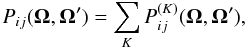
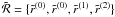
For simplicity, the decomposition method is presented for a redistribution matrix of the
form  (1)where
PR is the Rayleigh phase matrix (see e.g. Chandrasekhar 1950; Stenflo 1994) (see also LL04 p. 202 or the Appendix). In Sect. 5 we show how to extend the results obtained with
Eq. (1) to the redistribution matrix given
in Eq. (20) proposed by Bommier (1997a, henceforth VB matrix)1. The scattering problem considered here is simpler than the Hanle
effect problem investigated in HF09, but more explicit results are obtained. Our results can
be applied to pure resonance scattering, but also to the Hanle effect, if the magnetic field
is microturbulent.
(1)where
PR is the Rayleigh phase matrix (see e.g. Chandrasekhar 1950; Stenflo 1994) (see also LL04 p. 202 or the Appendix). In Sect. 5 we show how to extend the results obtained with
Eq. (1) to the redistribution matrix given
in Eq. (20) proposed by Bommier (1997a, henceforth VB matrix)1. The scattering problem considered here is simpler than the Hanle
effect problem investigated in HF09, but more explicit results are obtained. Our results can
be applied to pure resonance scattering, but also to the Hanle effect, if the magnetic field
is microturbulent.
The organization of the paper is as follows. In Sect. 2 we show how to express the Rayleigh phase matrix elements in terms of
irreducible tensors , simply related to the  . In Sect. 3 we show how to decompose the Stokes parameters
I and Q into four irreducible components
(K = Q = 0,
K = 2,Q = 0,1,2). The
components with Q = 1,2 come from the angle-dependence of
the PRD function
r(ν,ν′,Θ).
A transfer equation for the components is
established in Sect. 4. In Sect. 5 we generalize the results established in the preceding sections to the
full VB matrix and to the Hanle effect with a microturbulent magnetic field. We propose in
Sect. 6 an approximation of the single scattering
type for the polarization. Some concluding remarks on numerical aspects are presented in
Sect. 7. An Appendix contains some technical details.
. In Sect. 3 we show how to decompose the Stokes parameters
I and Q into four irreducible components
(K = Q = 0,
K = 2,Q = 0,1,2). The
components with Q = 1,2 come from the angle-dependence of
the PRD function
r(ν,ν′,Θ).
A transfer equation for the components is
established in Sect. 4. In Sect. 5 we generalize the results established in the preceding sections to the
full VB matrix and to the Hanle effect with a microturbulent magnetic field. We propose in
Sect. 6 an approximation of the single scattering
type for the polarization. Some concluding remarks on numerical aspects are presented in
Sect. 7. An Appendix contains some technical details.
2. Representation of the Rayleigh phase matrix elements
We consider a plane-parallel atmosphere, cylindrically symmetrical along the normal to the surface. No incident beam or deterministic magnetic field is there to break the symmetry. The primary source of photons is unpolarized. Since there is no magnetic field, Stokes V is zero. The polarized radiation field is cylindrically symmetrical (i.e. independent of the azimuthal angle χ of the ray direction) and can be described by the two Stokes parameters I and Q2, if the direction chosen for the measure of the linear polarization is parallel or perpendicular to the solar limb. In the Rayleigh phase matrix (see e.g. the Appendix) we retain the elements that are not cylindrically symmetrical because the redistribution function depends on the scattering angle Θ. In contrast, when dealing with monochromatic scattering, complete frequency redistribution, and angle-averaged PRD, these terms are needed only if the medium is not cylindrically symmetrical (Chandrasekhar 1950).
The elements of the full 4 × 4 Rayleigh phase matrix
PR(Ω,Ω′)
can be written as (see e.g. Bommier 1997a; LL04)
 (2)where
  (3)The notation
∗ stands for complex
conjugate. Explicit expressions of the tensors
(3)The notation
∗ stands for complex
conjugate. Explicit expressions of the tensors  can be found in LL04 (p. 211).
They satisfy the conjugation property
can be found in LL04 (p. 211).
They satisfy the conjugation property 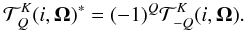 (4)They can be written as
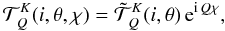 (5)where θ
and χ are the polar angles of the direction Ω. We
stress that
(5)where θ
and χ are the polar angles of the direction Ω. We
stress that  is in general a complex number. It depends on
θ and i but also on the reference angle
γ, which determines the reference direction for the measure of
Q. Here we use γ = 0. For a given point on the solar
disk, this choice corresponds to positive Stokes Q in the direction
perpendicular to the solar disk at the nearest point on the limb.
is in general a complex number. It depends on
θ and i but also on the reference angle
γ, which determines the reference direction for the measure of
Q. Here we use γ = 0. For a given point on the solar
disk, this choice corresponds to positive Stokes Q in the direction
perpendicular to the solar disk at the nearest point on the limb.
As U and V are zero for the problem at hand,
i takes only the values 0 and 1 and K the values 0 and
2. When in addition γ = 0, the tensors are real. It is then easy to check that
 (6)Inserting Eq. (5) into Eq. (2) and using the property that the are real, we can rewrite
  (7)Regrouping
the two terms with the same value of |Q| (for Q ≠ 0)
and making use of Eq. (6), we obtain
(7)Regrouping
the two terms with the same value of |Q| (for Q ≠ 0)
and making use of Eq. (6), we obtain
![Mathematical equation: \begin{equation} P_{ij}(\bm \Omega,\bm \Omega')= \sum_{K, Q\ge 0}c_{Q} {\tilde{\mathcal T}}^K_Q(i,\theta){\tilde{\mathcal T}}^K_Q(j,\theta')\cos [Q(\chi-\chi')], \label{new_matrix} \end{equation}](/articles/aa/full_html/2010/14/aa15167-10/aa15167-10-eq58.png) (8)where
cQ = 2 − δ0Q.
Here δ0Q is the Kronecker symbol equal to 0
when Q ≠ 0 and to 1 when Q = 0. We have four terms in the
summation over K and Q corresponding to
K = Q = 0, K = 2,
Q = 0,1,2. In the Appendix we give the
usual expressions of the Rayleigh phase matrix elements and the expressions of the . It is
easy to check that the Rayleigh matrix elements can indeed be written as shown in Eq. (8).
(8)where
cQ = 2 − δ0Q.
Here δ0Q is the Kronecker symbol equal to 0
when Q ≠ 0 and to 1 when Q = 0. We have four terms in the
summation over K and Q corresponding to
K = Q = 0, K = 2,
Q = 0,1,2. In the Appendix we give the
usual expressions of the Rayleigh phase matrix elements and the expressions of the . It is
easy to check that the Rayleigh matrix elements can indeed be written as shown in Eq. (8).
3. Decomposition of the Stokes parameters
As the radiation field is cylindrically symmetrical, the Stokes parameters only depend on
the inclination θ with respect to the Z-axis. The
polarized transfer equation for I = I0 and
Q = I1 can be written in component form as
![Mathematical equation: \begin{equation} \mu{\partial I_i\over \partial \tau} =\varphi(x)\bigl[I_i(\tau,x,\mu) - S_i(\tau,x,\mu)\bigr],\quad i=0,1, \label{transfer_eq} \end{equation}](/articles/aa/full_html/2010/14/aa15167-10/aa15167-10-eq66.png) (9)with
μ = cosθ. Here, τ is the line optical
depth defined by
dτ = −kldz,
where kl is the frequency-averaged line
absorption coefficient and ϕ(x) the normalized line
absorption coefficient. Henceforth, frequencies x are measured in Doppler
width units with zero at line center. The Doppler broadening is assumed to be
depth-independent. Here for simplicity we ignore the continuum absorption, emission, and
polarization. The source term is given by
(9)with
μ = cosθ. Here, τ is the line optical
depth defined by
dτ = −kldz,
where kl is the frequency-averaged line
absorption coefficient and ϕ(x) the normalized line
absorption coefficient. Henceforth, frequencies x are measured in Doppler
width units with zero at line center. The Doppler broadening is assumed to be
depth-independent. Here for simplicity we ignore the continuum absorption, emission, and
polarization. The source term is given by  (10)with
dΩ′ = sinθ′dθ′dχ′.
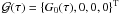
To avoid unnecessary complications we assume that the primary source is unpolarized; i.e.,
only the component G0(τ) is non zero. The
handling of a polarized primary source is described in HF07. We recall that
(10)with
dΩ′ = sinθ′dθ′dχ′.
To avoid unnecessary complications we assume that the primary source is unpolarized; i.e.,
only the component G0(τ) is non zero. The
handling of a polarized primary source is described in HF07. We recall that  (11)Introducing Eq. (8) into Eq. (10), we observe that the components
Si can be written as
(11)Introducing Eq. (8) into Eq. (10), we observe that the components
Si can be written as 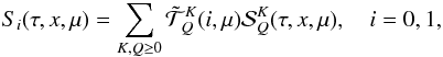 (12)with
 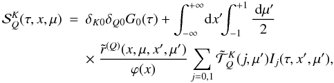 (13)and
![Mathematical equation: \begin{eqnarray} \tilde r^{(Q)}(x,\mu,x',\mu')= \frac{c_Q}{2\pi}\int_0^{2\pi}\!\!\!r(x,\mu,x',\mu',\chi-\chi') \cos [Q(\chi-\chi')]{\md}(\chi-\chi'). \label{fourier_coeff} \end{eqnarray}](/articles/aa/full_html/2010/14/aa15167-10/aa15167-10-eq80.png) (14)The
functions
(14)The
functions  are the azimuthal
Fourier coefficients of order 0, 1, and 2 of the PRD function
r(x,x′,Θ).
Plots of
are the azimuthal
Fourier coefficients of order 0, 1, and 2 of the PRD function
r(x,x′,Θ).
Plots of  versus x can be found in Domke & Hubeny (1988) for some choices of
μ, x′, μ′, and
Q. The numerical method introduced in Faurobert (1987) also employs three azimuthal averages of
r(x,x′,Θ),
but the weighting factors for Q = 1,2 are different.
Expansions of the redistribution functions rII and
rIII in Legendre polynomials have also been employed for
calculating Stokes I and Stokes Q (Mckenna 1985), although the frequency dependence of the Fourier expansion
coefficients have better numerical properties than the Legendre expansion coefficients,
which have sharp cusps and discontinuities in their derivatives (Domke & Hubeny 1988; see also in Milkey et al. 1975 the remark by
D. Hummer).
versus x can be found in Domke & Hubeny (1988) for some choices of
μ, x′, μ′, and
Q. The numerical method introduced in Faurobert (1987) also employs three azimuthal averages of
r(x,x′,Θ),
but the weighting factors for Q = 1,2 are different.
Expansions of the redistribution functions rII and
rIII in Legendre polynomials have also been employed for
calculating Stokes I and Stokes Q (Mckenna 1985), although the frequency dependence of the Fourier expansion
coefficients have better numerical properties than the Legendre expansion coefficients,
which have sharp cusps and discontinuities in their derivatives (Domke & Hubeny 1988; see also in Milkey et al. 1975 the remark by
D. Hummer).
At disk center the heliocentric angle θ is zero, therefore cosΘ is independent of the azimuth of the scattering angle (see Eq. (11)), r(x,x′,Θ) is cylindrically symmetrical, and the azimuthal Fourier components r(Q) with Q = 1,2 are zero.
The formal solution of Eq. (9) shows that
the components Ii(τ,x,μ) have
a decomposition similar to Eq. (12) (for
details see HF07), which can be written as 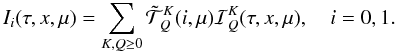 (15)Using the
expressions of the
(15)Using the
expressions of the  given in
Eq. (A.6), one finds
given in
Eq. (A.6), one finds 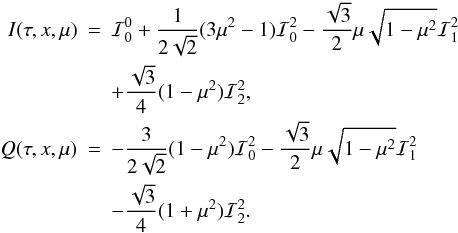 (16)The
same expansion holds for the source terms S0 and
S1 (see Eq. (12)). All the and
are
functions of τ, x, and μ. We show below
how to calculate them. We already note here that the components
(16)The
same expansion holds for the source terms S0 and
S1 (see Eq. (12)). All the and
are
functions of τ, x, and μ. We show below
how to calculate them. We already note here that the components  and
and  ,
Q = 1,2 are zero for μ = 1. This
implies that Stokes Q is zero at disk center.
,
Q = 1,2 are zero for μ = 1. This
implies that Stokes Q is zero at disk center.
4. Radiative transfer equations for the irreducible components
By introducing the decompositions of Si and
Ii (see Eqs. (12) and (15)) into
Eq. (9), we see that the components
 satisfy a transfer equation
similar to Eq. (9) with a source term
satisfy a transfer equation
similar to Eq. (9) with a source term
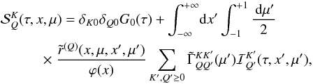 (17)where
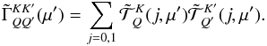 (18)The coefficients
 are given in the Appendix. Some of them are identical to the modulus of the multipole
coupling coefficients
ΓKQ,K′Q′
in LL04 (Appendix A.20), but differences occur because here the summation is over
j = 0,1. The dependence of
are given in the Appendix. Some of them are identical to the modulus of the multipole
coupling coefficients
ΓKQ,K′Q′
in LL04 (Appendix A.20), but differences occur because here the summation is over
j = 0,1. The dependence of  on μ only comes
from azimuthal Fourier coefficients of the redistribution function.
on μ only comes
from azimuthal Fourier coefficients of the redistribution function.
It is convenient to regroup the components into a 4-component vector
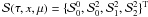 . When combining the formal solution
of the transfer equation for the with
Eq. (17), we obtain for the vector
. When combining the formal solution
of the transfer equation for the with
Eq. (17), we obtain for the vector
 an integral equation which may be
written as
an integral equation which may be
written as 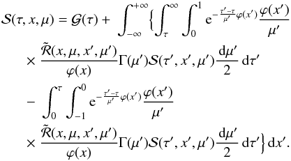 (19)For
simplicity we have assumed that we are dealing with a semi-infinite medium. Here
(19)For
simplicity we have assumed that we are dealing with a semi-infinite medium. Here
 is the primary source term,
 a diagonal matrix,
 , and Γ a full 4 × 4 matrix with elements
 . For symmetry it has only 10
different elements (see the Appendix).
. For symmetry it has only 10
different elements (see the Appendix).
When the frequency redistribution function is of the form
r(x,x′) (complete frequency
redistribution or angle-averaged PRD), only  and
and  are non zero. Moreover, they are
independent of μ. One recovers a standard decomposition in which the source
vector is described by a 2-component vector depending only on optical depth and, for PRD,
also on frequency. In Rees (1978) or Faurobert (1987), the starting point of the decomposition
is a factorization of the Rayleigh phase matrix of the form
PR(μ,μ′) = A(μ)AT(μ′),
where T stands for transpose. This type of factorization was first proposed by Sekara (1963). The choice of the matrix
A is not unique (see e.g. Van de Hulst 1980; Ivanov 1995). For
complete frequency redistribution, Omont et al.
(1973) (also Dumont et al. 1973) use an
expansion of the source term in irreducible components with
K = 0,2 and Q = 0.
are non zero. Moreover, they are
independent of μ. One recovers a standard decomposition in which the source
vector is described by a 2-component vector depending only on optical depth and, for PRD,
also on frequency. In Rees (1978) or Faurobert (1987), the starting point of the decomposition
is a factorization of the Rayleigh phase matrix of the form
PR(μ,μ′) = A(μ)AT(μ′),
where T stands for transpose. This type of factorization was first proposed by Sekara (1963). The choice of the matrix
A is not unique (see e.g. Van de Hulst 1980; Ivanov 1995). For
complete frequency redistribution, Omont et al.
(1973) (also Dumont et al. 1973) use an
expansion of the source term in irreducible components with
K = 0,2 and Q = 0.
In the direction μ = 1, the Fourier azimuthal components
 and
and
 are zero, as pointed
out above. Therefore only the components ,
are zero, as pointed
out above. Therefore only the components ,  and ,
and ,  are non zero. Setting
μ = 1 in Eq. (16), one
recovers Stokes Q = 0 at disk center, in agreement with the cylindrical
symmetry of the problem. Equation (16) shows
also that the contributions of
are non zero. Setting
μ = 1 in Eq. (16), one
recovers Stokes Q = 0 at disk center, in agreement with the cylindrical
symmetry of the problem. Equation (16) shows
also that the contributions of  to Stokes
I and Q go to zero when approaching the limb.
to Stokes
I and Q go to zero when approaching the limb.
5. General PRD polarization matrix
The elements of the VB redistribution matrix for a two-level atom with unpolarized ground
level, may be written as ![Mathematical equation: \begin{eqnarray} & &\hspace*{-2.2mm} R_{ij}(x,x',\Theta)=\sum_{K=0,2}\bigl[\alpha r_{\rm II}(x,x',\Theta)\nonumber\\ \label{redmat_gene} & &\hspace*{6mm} +~ [\beta^{(K)}-\alpha]r_{\rm III}(x,x',\Theta)\bigr]W_K P^{(K)}_{ij}({\bm \Omega},{\bm \Omega'}),\ i,j=0,1. \end{eqnarray}](/articles/aa/full_html/2010/14/aa15167-10/aa15167-10-eq125.png) (20)The
(20)The
 are defined in
Eq. (3) and given in the Appendix. For
K = 0,
are defined in
Eq. (3) and given in the Appendix. For
K = 0,  and the other elements are
zero. The coefficient W0 is equal to one and
W2 is an atomic depolarization factor depending on the angular
momenta Jl and Ju of the lower and
upper levels of the transition. It is equal to one for a normal Zeeman triplet
(Jl = 0, Ju = 1). Otherwise, it is
smaller than unity. Values of W2 for different values of
Jl and Ju can be found in LL04
(p. 515). The coefficients α and
β(K) are branching ratios:
and the other elements are
zero. The coefficient W0 is equal to one and
W2 is an atomic depolarization factor depending on the angular
momenta Jl and Ju of the lower and
upper levels of the transition. It is equal to one for a normal Zeeman triplet
(Jl = 0, Ju = 1). Otherwise, it is
smaller than unity. Values of W2 for different values of
Jl and Ju can be found in LL04
(p. 515). The coefficients α and
β(K) are branching ratios: 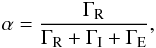 (21)and
 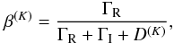 (22)with ΓR the
upper level spontaneous deexcitation radiative rate, ΓI and ΓE
inelastic and elastic collisions rates and D(K)
a collisional depolarization rate such that D(0) = 0. For more
detail see Bommier (1997a).
(22)with ΓR the
upper level spontaneous deexcitation radiative rate, ΓI and ΓE
inelastic and elastic collisions rates and D(K)
a collisional depolarization rate such that D(0) = 0. For more
detail see Bommier (1997a).
When a microturbulent magnetic field is present in the medium, the elements of the scattering phase matrix may be written as in Eq. (20) with WK replaced by WKμK (see e.g. LL04, p. 215). The coefficient μ0 is equal to one. The coefficient μ2 depends on the magnetic field vector probability density function. Expressions of μ2 for a magnetic field with a single field strength value, an isotropic, or horizontal angular distribution can be found in Stenflo (1994) (see also LL04).
We easily see that the decomposition presented in the preceding sections is still valid.
The matrix  in Eq. (19) remains a diagonal matrix. Its four elements
 may
be written as
may
be written as ![Mathematical equation: \begin{eqnarray} \tilde{\mathcal R}^0_0& = &\alpha \tilde r^{(0)}_{\rm II} + (\beta ^{(0)} -\alpha)\tilde r^{(0)}_{\rm III},\\ \label{matrix_rgene} \tilde{\mathcal R}^2_Q& = &W_2\mu_2\left[\alpha \tilde r^{(Q)}_{\rm II} + (\beta ^{(2)} -\alpha)\tilde r^{(Q)}_{\rm III}\right] , \quad Q=0,1,2. \end{eqnarray}](/articles/aa/full_html/2010/14/aa15167-10/aa15167-10-eq150.png) Since
the Hanle effect only acts at line center, the coefficient μ2
should be set to unity outside the line core.
Since
the Hanle effect only acts at line center, the coefficient μ2
should be set to unity outside the line core.
6. Approximate expressions for the irreducible components
The linear polarization observed in the second solar spectrum is never more than a few
percent. This implies that the components ,
Q = 0,1,2 are significantly smaller
than the component , the
dominant term of Stokes I (see Eq. (16)). The same behavior holds for the components
.
Neglecting the components
(Q = 0,1,2) in Eq. (17), we obtain for each component
 the approximate expression
 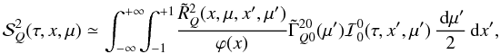 (25)where
is the solution of a non-LTE, but
non-polarized, radiative transfer equation with partial frequency redistribution. For
consistency, one should use
(25)where
is the solution of a non-LTE, but
non-polarized, radiative transfer equation with partial frequency redistribution. For
consistency, one should use  for
the redistribution function. The expression proposed in Eq. (25) is of the last scattering approximation type (see e.g. Faurobert 1987, 1988; Frisch et al. 2009; Anusha et al. 2010). The functions
for
the redistribution function. The expression proposed in Eq. (25) is of the last scattering approximation type (see e.g. Faurobert 1987, 1988; Frisch et al. 2009; Anusha et al. 2010). The functions
 are defined in Eq. (24), and the coefficients
 can be found in the
Appendix. The approximate expressions of
can be found in the
Appendix. The approximate expressions of  can then be used to calculate
approximate values of the components by solving
a simple transfer equation. An Eddington-Barbier approximation may give the right order of
magnitude for the , provided
the have a
variation with optical depth that is not too far from linear. For PRD, this condition may be
far from being satisfied, in particular near line center.
can then be used to calculate
approximate values of the components by solving
a simple transfer equation. An Eddington-Barbier approximation may give the right order of
magnitude for the , provided
the have a
variation with optical depth that is not too far from linear. For PRD, this condition may be
far from being satisfied, in particular near line center.
7. Concluding remarks
In this paper we consider Rayleigh scattering with angle-dependent PRD effects in a
cylindrically symmetrical medium. Because of this symmetry the Stokes parameters
I and Q are also cylindrically symmetrical. That
frequency redistribution depends on the scattering angle does not modify this property. We
show that I and Q can be decomposed into four components
(K = Q = 0,
K = 2,Q = 0,1,2),
which are also cylindrically symmetrical. They satisfy a transfer equation similar to the
transfer equation for I and Q. In both equations the
source terms depend on the ray inclination θ, so one may wonder what has
been gained in this decomposition.
First, as shown in Eq. (16), this decomposition allows one to separate the contributions with Q = 0 coming from the cylindrically symmetric part of the redistribution function from the contributions corresponding to Q ≠ 0, which are created by the departure from cylindrical symmetry. These components go to zero at disk center, but they contribute to the polarization near the limb. One can thus easily evaluate errors that are made when departures from cylindrical symmetry in the redistribution matrix are ignored.
Another interesting property of the decomposition in irreducible components is that the
source term in the transfer equations for
has a much simpler form than the
source terms SI and SQ for the
Stokes parameters I and Q. There is no integration over
the azimuthal angle of the incident radiation, and the dependence on the inclination angle
θ of the scattered radiation comes from the azimuthal Fourier
coefficients  only and not from both the
frequency redistribution functions and scattering phase matrix. A consequence of this
simplification is that the set of integral equations for the four components
can be
solved by an ALI (accelerated lambda iteration) method as will be shown in a forthcoming
paper. Of course, compared to angle-averaged PRD, the dependence on the inclination angle
θ introduces an additional numerical complexity since a fairly large
number of values of the inclination angles of the incident and scattered beams are needed
for a correct description of the azimuthal Fourier coefficients
only and not from both the
frequency redistribution functions and scattering phase matrix. A consequence of this
simplification is that the set of integral equations for the four components
can be
solved by an ALI (accelerated lambda iteration) method as will be shown in a forthcoming
paper. Of course, compared to angle-averaged PRD, the dependence on the inclination angle
θ introduces an additional numerical complexity since a fairly large
number of values of the inclination angles of the incident and scattered beams are needed
for a correct description of the azimuthal Fourier coefficients  and
and  . We recall that ALI methods,
which are of the operator splitting type, are quite efficient in solving polarized transfer
equations. They have been developed in the past 25 years, first for complete frequency
redistribution, but have then been extended to PRD problems with angle-averaged
redistribution functions. They have been employed for Rayleigh scattering, but also for the
Hanle effect (see the review by Nagendra & Sampoorna
2009). With the decomposition proposed in the present paper (see also HF09), it
becomes possible to generalize ALI methods to angle-dependent PRD. Preliminary numerical
results confirm that, for Rayleigh scattering, angle-dependent and angle-averaged PRD give
essentially the same value of Stokes I. For Stokes Q there
are some differences, but they seem to remain small (15% at most for the ratio
Q/I). In contrast, for the Hanle
effect the angle-averaged and angle-dependent PRD functions yield significantly different
Stokes Q profiles (Nagendra et al.
2002).
. We recall that ALI methods,
which are of the operator splitting type, are quite efficient in solving polarized transfer
equations. They have been developed in the past 25 years, first for complete frequency
redistribution, but have then been extended to PRD problems with angle-averaged
redistribution functions. They have been employed for Rayleigh scattering, but also for the
Hanle effect (see the review by Nagendra & Sampoorna
2009). With the decomposition proposed in the present paper (see also HF09), it
becomes possible to generalize ALI methods to angle-dependent PRD. Preliminary numerical
results confirm that, for Rayleigh scattering, angle-dependent and angle-averaged PRD give
essentially the same value of Stokes I. For Stokes Q there
are some differences, but they seem to remain small (15% at most for the ratio
Q/I). In contrast, for the Hanle
effect the angle-averaged and angle-dependent PRD functions yield significantly different
Stokes Q profiles (Nagendra et al.
2002).
The cylindrical symmetry of I and Q can be proven for an angle-dependent partial frequency redistribution by expanding the solution of the integral equation for the Stokes parameters source vector in a Neumann series.
Acknowledgments
The author is grateful to K. N. Nagendra, M. Sampoorna and J. O. Stenflo for helpful remarks and to an anonymous referee for constructive comments.
References
- Anusha, L. S., Nagendra, K. N., Stenflo, J. O., et al. 2010, ApJ, 718, 988 [NASA ADS] [CrossRef] [Google Scholar]
- Bommier, V. 1997a, A&A, 328, 706 [NASA ADS] [Google Scholar]
- Bommier, V. 1997b, A&A, 328, 726 [NASA ADS] [Google Scholar]
- Chandrasekhar, S. 1950, Radiative Transfer (Dover) [Google Scholar]
- Domke, H., & Hubeny, I. 1988, ApJ, 213, 296 [Google Scholar]
- Dumont, S., Omont, A., & Pecker, J.-C. 1973, Sol. Phys., 28, 271 [NASA ADS] [CrossRef] [Google Scholar]
- Faurobert, M. 1987, A&A, 178, 269 [NASA ADS] [Google Scholar]
- Faurobert, M. 1988, A&A, 194, 268 [NASA ADS] [Google Scholar]
- Faurobert-Scholl, M. 1996, Sol. Phys., 164, 79 [NASA ADS] [CrossRef] [Google Scholar]
- Frisch, H. 2007, A&A, 476, 665 (HF07) [NASA ADS] [CrossRef] [EDP Sciences] [Google Scholar]
- Frisch, H. 2009, in Solar Polarization V, ed. S. V. Berdyugina, K. N. Nagendra, & R. Ramelli (San Francisco: ASP), ASP Conf. Ser., 405, 87 (HF09) [Google Scholar]
- Frisch, H., Anusha, L. S., Sampoorna, M., & Nagendra, K. N. 2009, A&A, 501, 335 [NASA ADS] [CrossRef] [EDP Sciences] [Google Scholar]
- Gandorfer, A. 2000, The Second Solar Spectrum, Vol. I: 4625 Å to 6995 Å (Zurich:VdF), ISBN No. 3 7281 2764 7 [Google Scholar]
- Gandorfer, A. 2002, The Second Solar Spectrum, Vol. II: 3910 Å to 4630 Å (Zurich:VdF), ISBN No. 3 7281 2844 4 [Google Scholar]
- Gandorfer, A. 2005, The Second Solar Spectrum, Vol. III: 3160 Å to 3915 Å (Zurich:VdF), ISBN No. 3 7281 3018 4 [Google Scholar]
- Hummer, D. 1962, MNRAS, 125, 21 [NASA ADS] [CrossRef] [Google Scholar]
- Ivanov, V. V. 1991, in Stellar Atmospheres: Beyond Classical Models, NATO ASI Series C 341, ed. L. Crivellari, I. Hubeny, & D. G. Hummer (Dordrecht: Kluwer), 81 [Google Scholar]
- Ivanov, V. V. 1995, A&A, 303, 609 [NASA ADS] [Google Scholar]
- Landi Degl’Innocenti, E. 1984, Sol. Phys., 91, 1 [NASA ADS] [CrossRef] [Google Scholar]
- Landi Degl’Innocenti, E., & Landolfi, M. 2004, Polarization in Spectral Lines (Kluwer Academic Publishers) (LL04) [Google Scholar]
- McKenna, S. J. 1985, Ap&SS, 108, 31 [NASA ADS] [CrossRef] [Google Scholar]
- Milkey, R. W., Shine, R. A., & Mihalas, D. 1975, ApJ, 202, 250 [NASA ADS] [CrossRef] [Google Scholar]
- Nagendra, K. N., & Sampoorna, M. 2009, in Solar Polarization V, ed. S. V. Berdyugina, K. N. Nagendra, & R. Ramelli (San Francisco: ASP), ASP Conf. Ser., 405, 261 [Google Scholar]
- Nagendra, K. N., Frisch, H., & Faurobert, M. 2002, A&A, 395, 305 [NASA ADS] [CrossRef] [EDP Sciences] [Google Scholar]
- Omont, A., Smith, E. W., & Cooper, J. 1972, ApJ, 175, 185 [Google Scholar]
- Omont, A., Smith, E. W., & Cooper, J. 1973, ApJ, 182, 283 [NASA ADS] [CrossRef] [Google Scholar]
- Rees, D. E. 1978, Publ. Astr. Soc. Japan, 30, 455 [NASA ADS] [Google Scholar]
- Rees, D. E., & Saliba, G. J. 1982, A&A, 115, 1 [NASA ADS] [Google Scholar]
- Sampoorna, M., Nagendra, K. N., & Stenflo, J. O. 2007, ApJ, 670, 1485 [NASA ADS] [CrossRef] [Google Scholar]
- Sekara, Z. 1963, Rand Corporation Memo. R-413-PR [Google Scholar]
- Stenflo, J. O. 1976, A&A, 46, 61 [NASA ADS] [Google Scholar]
- Stenflo, J. O. 1982, Sol. Phys., 80, 209 [NASA ADS] [CrossRef] [Google Scholar]
- Stenflo, J. O. 1994, Solar Magnetic Fields (Kluwer Academic Publishers) [Google Scholar]
- Trujillo Bueno, J., Shchukina N., & Asensio Ramos, A. 2004, Nature, 430, 326 [Google Scholar]
- Van de Hulst, H. C. 1980, Multiple light scattering, Tables, Formulas and Applications (Academic Press) [Google Scholar]
Appendix A: Rayleigh phase matrix, spherical tensors, and coefficients 
The Rayleigh phase matrix can be written as (Stenflo
1994; see also LL04) 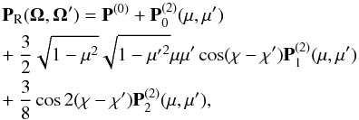 (A.1)where
![Mathematical equation: \appendix \setcounter{section}{1} \begin{eqnarray} {\bf P}^{(0)}=\left[ \begin{array}{cc} 1&0\\ 0&0 \end{array}\right], \label{pisotrope} \end{eqnarray}](/articles/aa/full_html/2010/14/aa15167-10/aa15167-10-eq164.png) (A.2)
(A.2)![Mathematical equation: \appendix \setcounter{section}{1} \begin{eqnarray} {\bf P}^{(2)}_0=\frac{1}{8}\left[ \begin{array}{cc} (1-3\mu ^2)(1-3{\mu'}^2)&3(1-3\mu ^2)(1-{\mu'}^2)\\ 3(1-\mu ^2)(1-3{\mu'}^2)&9(1-\mu ^2)(1-{\mu'}^2) \end{array}\right], \label{p20} \end{eqnarray}](/articles/aa/full_html/2010/14/aa15167-10/aa15167-10-eq165.png) (A.3)
(A.3)![Mathematical equation: \appendix \setcounter{section}{1} \begin{eqnarray} {\bf P}^{(2)}_1=\left[ \begin{array}{cc} 1&1\\ 1&1 \end{array}\right], \label{p21} \end{eqnarray}](/articles/aa/full_html/2010/14/aa15167-10/aa15167-10-eq166.png) (A.4)
(A.4)![Mathematical equation: \appendix \setcounter{section}{1} \begin{eqnarray} {\bf P}^{(2)}_2=\left[ \begin{array}{cc} (1-\mu ^2)(1-{\mu'}^{2})& -(1-\mu ^2)(1+{\mu'}^{2})\\ -(1+\mu ^2)(1-{\mu'}^{2})&(1+\mu ^2)(1+{\mu'}^{2}) \end{array}\right]. \label{p22} \end{eqnarray}](/articles/aa/full_html/2010/14/aa15167-10/aa15167-10-eq167.png) (A.5)For
i = 0,1 and the reference angle
γ = 0, the
(A.5)For
i = 0,1 and the reference angle
γ = 0, the  introduced in Sect. 2 of the text are given by the modulus of the spherical tensors
 given in LL04 (p. 211).
They may be written as
given in LL04 (p. 211).
They may be written as 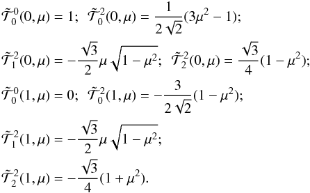 (A.6)The
coefficients
(A.6)The
coefficients  introduced in the text
are defined by
introduced in the text
are defined by 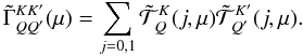 (A.7)They satisfy the
symmetry
(A.7)They satisfy the
symmetry  , so only 10 of them are
different. They are
, so only 10 of them are
different. They are 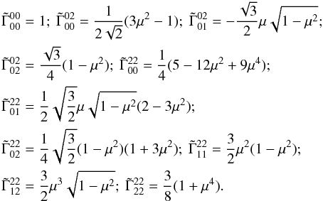 (A.8)
(A.8)
All Figures
|
Fig. 1 Atmospheric reference system. The directions Ω and Ω′ are defined by their polar angles (θ,χ) and (θ′,χ′) and Θ is the scattering angle. The Z-axis is along the outside normal to the atmosphere. |
| In the text | |
Current usage metrics show cumulative count of Article Views (full-text article views including HTML views, PDF and ePub downloads, according to the available data) and Abstracts Views on Vision4Press platform.
Data correspond to usage on the plateform after 2015. The current usage metrics is available 48-96 hours after online publication and is updated daily on week days.
Initial download of the metrics may take a while.