| Issue |
A&A
Volume 522, November 2010
|
|
|---|---|---|
| Article Number | A42 | |
| Number of page(s) | 12 | |
| Section | Interstellar and circumstellar matter | |
| DOI | https://doi.org/10.1051/0004-6361/201015149 | |
| Published online | 29 October 2010 | |
Research Note
Chemistry in disks⋆
IV. Benchmarking gas-grain chemical models with surface reactions
1
Max Planck Institute for Astronomy,
Königstuhl 17,
69117
Heidelberg,
Germany
e-mail: semenov@mpia.de
2
Université de Bordeaux, Observatoire Aquitain des Sciences de
l’Univers, 2 rue de l’Observatoire, BP 89, 33271
Floirac Cedex,
France
3
CNRS, UMR 5804, Laboratoire d’Astrophysique de Bordeaux, 2 rue de
l’Observatoire, BP
89, 33271
Floirac Cedex,
France
4
Max-Planck-Institut für Radioastronomie,
Auf dem Hügel 69,
53121
Bonn,
Germany
5
IRAM, 300 rue de la piscine, 38406
Saint Martin d’Hères,
France
6
Astrophysikalisches Institut und Universitäts-Sternwarte,
Schillergässchen
2–3, 07745
Jena,
Germany
Received: 4 June 2010
Accepted: 24 June 2010
Context. We describe and benchmark two sophisticated chemical models developed by the Heidelberg and Bordeaux astrochemistry groups.
Aims. The main goal of this study is to elaborate on a few well-described tests for state-of-the-art astrochemical codes covering a range of physical conditions and chemical processes, in particular those aimed at constraining current and future interferometric observations of protoplanetary disks.
Methods. We considered three physical models: a cold molecular cloud core, a hot core, and an outer region of a T Tauri disk. Our chemical network (for both models) is based on the original gas-phase osu_03_2008 ratefile and includes gas-grain interactions and a set of surface reactions for the H-, O-, C-, S-, and N-bearing molecules. The benchmarking was performed with the increasing complexity of the considered processes: (1) the pure gas-phase chemistry, (2) the gas-phase chemistry with accretion and desorption, and (3) the full gas-grain model with surface reactions. The chemical evolution is modeled within 109 years using atomic initial abundances with heavily depleted metals and hydrogen in its molecular form.
Results. The time-dependent abundances calculated with the two chemical models are essentially the same for all considered physical cases and for all species, including the most complex polyatomic ions and organic molecules. This result, however, required a lot of effort to make all necessary details consistent through the model runs, e.g., definition of the gas particle density, density of grain surface sites, or the strength and shape of the UV radiation field.
Conclusions. The reference models and the benchmark setup, along with the two chemical codes and resulting time-dependent abundances are made publicly available on the internet. This will facilitate and ease the development of other astrochemical models and provide nonspecialists with a detailed description of the model ingredients and requirements to analyze the cosmic chemistry as studied, e.g., by (sub-) millimeter observations of molecular lines.
Key words: astrochemistry / molecular processes / molecular data / methods: numerical / ISM: molecules / protoplanetary disks
Figures 1–5 and Tables 1–3 are only available in electronic form at http://www.aanda.org
© ESO, 2010
1. Introduction
Astrochemistry plays an important role in our understanding of the star- and planet-formation processes across the Universe (e.g., Bergin et al. 2007; Kennicutt 1998; Solomon & Vanden Bout 2005; van Dishoeck & Blake 1998). Molecules serve as unique probes of physical conditions, evolutionary stage, kinematics, and chemical complexity. In astrophysical objects, molecular concentrations are usually hard to predict analytically as it involves a multitude of chemical processes that almost never reach a chemical steady-state. Consequently, to calculate molecular concentrations, one has to specify initial conditions and abundances and to solve a set of chemical kinetics equations.
Since the first seminal studies on chemical modeling of the interstellar medium (ISM) by Bates & Spitzer (1951), Herbst & Klemperer (1973), and Watson & Salpeter (1972), numerous chemical models of molecular clouds (e.g., Hasegawa et al. 1992), protoplanetary disks (e.g., Aikawa et al. 2002), shells around late-type stars (e.g., Agúndez & Cernicharo 2006), AGN tori (e.g., Meijerink et al. 2007), and planetary atmospheres (e.g., Gladstone et al. 1996) have been developed. These models are mainly based on three widely applied ratefiles: the UDFA (Umist Database For Astrochemistry1) (Millar et al. 1997; Le Teuff et al. 2000; Woodall et al. 2007), the OSU database (Ohio State University2) (Smith et al. 2004), and a network incorporated in the “Photo-Dissociation Region” code from Meudon3 (Le Petit et al. 2006). Recently another database of chemical reactions for the interstellar medium and planetary atmospheres, KIDA4, has been opened to the astrochemical community. The main aim of KIDA is to group all kinetic data to model the chemistry of these environments and to allow physico-chemists to upload their data onto the database and astrochemists to present their models. Several compilations of surface reactions have also been presented (e.g., Allen & Robinson 1977; Tielens & Hagen 1982; Hasegawa et al. 1992; Hasegawa & Herbst 1993; Garrod & Herbst 2006). The detailed physics and chemistry processes incorporated in the modern theoretical models allow predicting and, at last, fitting to the observational interferometric data, such as molecular line maps of protoplanetary disks and molecular clouds (e.g., Semenov et al. 2005; Dutrey et al. 2007; Goicoechea et al. 2009; Panić & Hogerheijde 2009; Henning et al. 2010). However, with the advent of forthcoming high-sensitivity, high-resolution instruments like ALMA, ELT, and JWST, the degree of complexity of these models will have to be increased and their foundations be critically re-evaluated to match the quality of the data (e.g., Asensio Ramos et al. 2007; Lellouch 2008; Semenov et al. 2008).
There are other difficulties with cosmochemical models. Apart from often poorly known physical properties of the object, its chemical modeling suffers from uncertainties in the reaction rates, of which only ≲ 10% have been accurately determined (see, e.g., Herbst 1980; Wakelam et al. 2006; Vasyunin et al. 2008). In contrast to these internal uncertainties, another major source of ambiguity is the lack of detailed description of chemical models that often incorporate different astrochemical ratefiles, initial abundances, dust grain properties, etc., thus making results hard to interpret and compare. It is thus essential to perform consistent benchmarking of various advanced chemical models under a variety of realistic physical conditions, in particular those encountered in protoplanetary disks. To the best of our knowledge, the only important benchmarking study attempted so far has focused on several PDR physico-chemical codes (Röllig et al. 2007).
The ultimate goal of present work is i) to provide a detailed description of our time-dependent sophisticated chemical codes; and ii) to establish a set of reference models covering a wide range of physical conditions, from a cold molecular cloud core to a hot corino and an outer region of a protoplanetary disk. In comparison with the PDR benchmark, our study is based on a more extended set of gas-grain and surface reactions. All the relevant software, figures, reaction network, and calculated abundances are available on the internet5.
The organization of the paper is the following. In Sect. 2, the two codes and the chemical network are presented in detail, along with our approach to calculating the reaction rates. In Sect. 3, we describe various benchmarking models, the physical conditions, and the initial chemical abundances. The benchmarking runs and their results are presented and compared in Sect. 4. Final conclusions are drawn in Sect. 5.
2. Chemical models
2.1. Heidelberg and Bordeaux chemical codes
In this study, we compare two chemical codes, “ALCHEMIC” and “NAUTILUS”, developed independently over the past several years by the Heidelberg and Bordeaux astrochemistry groups. Both codes have been intensively utilized in various studies of molecular cloud and protoplanetary disk chemistry, e.g. the influence of the reaction rate uncertainties on the results of chemical modeling of cores (Vasyunin et al. 2004; Wakelam et al. 2005, 2006) and disks (Vasyunin et al. 2008), modeling of the disk chemical evolution with turbulent diffusion (Semenov et al. 2006; Hersant et al. 2009), interpretation of interferometric data (Semenov et al. 2005; Dutrey et al. 2007; Schreyer et al. 2008; Henning et al. 2010), and predictions for ALMA (Semenov et al. 2008). Both codes are optimized to model time-dependent evolution of a large set of gas-phase and surface species linked through thousands of gas-phase, gas-grain, and surface processes. We find that both these codes have comparable performance, accuracy, and fast convergence speed thanks to advanced ODE and sparse matrix linear system solvers.
The Heidelberg “ALCHEMIC” code is written in Fortran 77 and based on the publicly available DVODPK (Differential Variable-coefficient Ordinary Differential equation solver with the Preconditioned Krylov method GMRES for the solution of linear systems) ODE package6. The full Jacobi matrix is generated automatically from the supplied chemical network to be used as a lefthand preconditioner. For astrochemical models dominated by reactions involving hydrogen, the Jacobi matrix is sparse (having ≲ 1% of non-zero elements); therefore, to solve the corresponding linearized system of equations, a high-performance sparse unsymmetric MA28 solver from the Harwell Mathematical Software Library7 is used. As ratefiles, both the recent OSU 06 and osu.2008 and the RATE 06 networks can be utilized. A typical run with relative and absolute accuracies of 10-5 and 10-15 for the full gas-grain network with surface chemistry (~650 species, ~7000 reactions) and 5 Myr of evolution takes only a few seconds of CPU time on the Xeon 2.8 GHz PC (with gfortran 4.3 compiler).
The Bordeaux “NAUTILUS” code is written in Fortran 90 and uses the LSODES (Livermore Solver for Ordinary Differential Equations with general Sparse Jacobian matrix) solver, part of ODEPACK8 (Hindmarsh 1983). “NAUTILUS” is adapted from the original gas-grain model of Hasegawa & Herbst (1993) and its subsequent evolutions made over the years at Ohio State University. The main differences with the OSU model rely on the numerical scheme and optimization (“NAUTILUS” is about 20 times faster), the possibility of computing 1D structures with diffusive transport, and the adaptation to disk physics and chemistry. The full Jacobian is computed from the chemical network without preconditioning. For historical reasons, only the OSU rate files are being used, although minor adjustments could permit extending this model to other networks. Similar performances with “ALCHEMIC” are achieved, where the same typical run of the full gas-grain network takes a few seconds on a standard desktop computer.
Below we explain how we model various gas-phase and surface reactions.
2.2. Modeling of chemical processes
Chemical codes numerically solve the equations of chemical kinetics describing the formation and destruction of molecules:  (1)
(1) (2)where ni and
  are the gas-phase and surface concentrations of the ith species (cm-3), klm and kl are the gas-phase reaction rates (in units of s-1 for the first-order kinetics and cm3 s-1 for the second-order kinetics),
  and
and  denote the accretion and desorption rates (s-1), and
  and
and  are surface reaction rates (cm3 s-1).
2.2.1. Gas-phase reactions
For the benchmarking, we utilize a recent osu_03_2008 gas-phase ratefile9. It incorporates the data for the 456 atomic, ionic, and molecular species involved in the 4389 gas-phase reactions. The corresponding reaction rates are calculated as follows, using the standard Arrhenius representation: 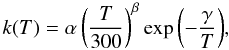 (3)where α is the value of the reaction rate at the room temperature of 300 K, the parameter β characterizes the temperature dependence of the rate, and γ is the activation barrier (in Kelvin). We utilize this expression for all gas-phase two-body processes, e.g. ion-molecular and neutral-neutral reactions.
For the cosmic ray and FUV ionization and dissociation the following prescriptions have been used.
Cosmic ray (CR) ionization & dissociation.
To calculate ionization and dissociation rates of chemical species by the cosmic ray particles, we utilize the following standard scaling expression:  (4)where ζCR = 1.3 × 10⁻¹⁷ s-1 is the adopted CR ionization rate. In all benchmarking models, any additional sources of ionization such as the X-ray stellar radiation and the decay of short-lived radionucleides (e.g., 26Al and 40K) are not considered. This small set of reactions includes ionization of relevant atoms and dissociation of molecular hydrogen. The same expression is used to compute photodissociation and ionization by the CR-induced FUV photons. Also, the CR- and UV-driven dissociation of surface species is calculated by the Eq. (4) (616 processes).
FUV photodissociation and ionization.
To calculate photoreaction rates through the environment, we adopt precomputed fits of van Dishoeck (1988) for a 1D plane-parallel slab, using the Draine FUV IS radiation field. Unlike in the PDR benchmarking study, the self-and mutual-shielding of CO and H2 against UV photodissociation are not taken into account for simplicity. The corresponding rate is calculated as  (5)where AV is the visual extinction (mag) and χ the unattenuated FUV flux expressed in units of the FUV interstellar radiation field χ0 of Draine (1978). We do not take the Lyα radiation into account as it requires sophisticated modeling of the radiation transport – a full-scale benchmarking study by itself (e.g., Pascucci et al. 2004; Röllig et al. 2007).
2.3. Gas-grain interactions
For simplicity, we assume that the dust grains are uniform spherical particles, with a radius of ag = 0.1μm, made of amorphous olivine, with density of ρd = 3 g cm-3 and a dust-to-gas mass ratio md / g = 0.01. The surface density of sites is Ns = 1.5 × 10¹⁵ sites cm-2, and the total number of sites per each grain is S = 1.885 × 10⁶. The dust and gas temperatures are assumed to be the same.
Gas-grain interactions start with the accretion of neutral molecules onto dust surfaces with a sticking efficiency of 100% (195 processes). Molecules are assumed to only physisorb on the grain surface (by van der Waals force) rather than by forming a chemical bond with the lattice (chemisorption). The rate of accretion of a gas-phase species i (cm-3 s-1) is given by  (6)where n(i) is the density of gas-phase species i (cm-3), and kacc(i) = σd ⟨ v(i) ⟩ nd the accretion rate. Here
  is the geometrical cross section of the grain with the radius ag, nd is the density of grains (cm-3) and ⟨ v(i) ⟩ is the thermal velocity of species i (cm s-1). The latter quantity is expressed as
  , with T being the gas temperature (K), mp = 1.66054 × 10⁻²⁴ g is the proton’s mass, μ(i) is the reduced mass of the molecule i (in atomic mass units), and kB = 1.38054 × 10⁻¹⁶ erg K-1 is the Boltzmann’s constant. All constants are summarized in Table 2.
In addition, electrons can stick to neutral grains, producing negatively charged grains. Atomic ions radiatively recombine on these negatively charged grains, leading to grain neutralization (13 reactions in total). The corresponding two-body reaction rate is calculated as  (7)where nH is the total hydrogen nucleus density (cm-3). This quantity is calculated by the expression
  (8)where ρ is the gas mass density (g cm-3), and μ = 1.43 the mean mass per hydrogen nucleus. Consequently, the density of grains nd is expressed as
  (9)We consider neither interactions of molecular ions with grains nor the photoelectric effect leading to positively charged grains.
In our simplified model used for benchmarking purposes, the surface molecules can leave the grain by only two mechanisms. First, they can desorb back into the gas phase when a grain is hit by a relativistic iron nucleus and heated for a short while up to several tens of Kelvin (160 reactions, cosmic-ray induced desorption). Second, in sufficiently warm regions, thermal desorption becomes efficient. The thermal desorption for the ith surface molecule is calculated by the Polanyi-Wigner equation:  (10)Here,
  is the characteristic vibrational frequency of the ith species, Edes its desorption energy (Kelvin), m the mass of the species, and Td the grain temperature. Desorption energies Edes are taken from Garrod & Herbst (2006). We do not distinguish between various thermal evaporation scenarios for different molecules, e.g. via “volcanic” or multilayer desorption (Collings et al. 2004).
The cosmic ray desorption rate is computed as suggested by Eq. (15) in Hasegawa & Herbst (1993). It is based on the assumption that a cosmic ray particle (usually an iron nucleus) deposits on average 0.4 MeV into a dust grain of the adopted radius, impulsively heating it to a peak temperature Tcrp = 70 K (see also Leger et al. 1985). The resulting rate is  (11)where kcrd is the thermal evaporation rate at 70 K times the fraction of the time the grain temperature stays close to 70 K. The fraction f is a ratio of a grain cooling timescale via desorption of molecules to the timescale of subsequent heating events (e.g., for a 0.1 μm silicate particle and the standard CR ionization rate 1.3 × 10⁻¹⁷ s-1 these timescales are ~10-5 s and ~3 × 10¹³ s, respectively). Other nonthermal desorption mechanisms (e.g., photodesorption) that can play important roles in chemistry of protoplanetary disks are not considered.
2.4. Surface reactions
Surface reactions (532 in the network) are treated in the standard rate approximation, assuming only Langmuir-Hinshelwood formation mechanism, as described, e.g., in Hasegawa et al. (1992). Surface species are only allowed to move from one surface site to another by thermal hopping. When two surface species find each other, they can recombine. We assume that the products do not leave the surface as the excess of energy produced by such a reaction will be immediately absorbed by the grain lattice, i.e. we did not include the desorption process proposed by Garrod et al. (2007).
Rate coefficients for surface reactions between species i and j are expressed as  (12)Here P is the probability for the reaction to occur. This parameter is 1 for an exothermic reaction without activation energy and 1 / 2 if the two reactants are the same type. For exothermic reactions with activation energy Ea (or endothermic reactions), this probability is
  , with α the branching ratio of the reaction (α = 1 / 3 if there are three reaction channels). In some cases, tunneling effects can increase this probability10. When this is the case, P is computed through the following formula (Hasegawa et al. 1992):
 ![\begin{equation} P = \alpha \exp\left[-2 (b/\hbar)(2 k_{\rm B} \mu(i) m_p E_{\rm a})^{1/2}\right] \end{equation}](/articles/aa/full_html/2010/14/aa15149-10/aa15149-10-eq86.png) (13)with b the barrier thickness (1 Å) and ħ the Planck constant times 2π (1.05459 × 10⁻²⁷ erg s-1).
(13)with b the barrier thickness (1 Å) and ħ the Planck constant times 2π (1.05459 × 10⁻²⁷ erg s-1).
The thermal diffusion rate of species i is  (14)Here kBTdiff is the activation energy of diffusion for the ith molecule.
The diffusion and desorption energies of a limited set of molecular species have already been derived (e.g., Katz et al. 1999; Bisschop et al. 2006; Öberg et al. 2007). Moreover, these energies depend on the type of the surface lattice and its structural properties (porosity, crystallinity, e.g., Acharyya et al. 2007; Thrower et al. 2009). While diffusion energy of a species must be lower than its desorption energy, the exact ratio is not well constrained for a majority of molecules in our network (except for H2, see Katz et al. 1999). Following Ruffle & Herbst (2000), we adopted the Tdiff / Tdes ratio of 0.77 for the all relevant species in the model.
It has been proposed that light surface species like H, H2 and isotopes can also quantum tunnel through a potential well of the surface site and thus be able to quickly scan the surface, greatly increasing the efficiency of surface recombination even at very low temperatures (e.g., Duley & Williams 1986; Hasegawa et al. 1992). However, according to the theoretical interpretation of Katz et al. (1999) tunneling of atomic hydrogen on amorphous surfaces does not occur. Therefore, it is not considered in our benchmarking study.
Finally, at very low influx of reacting species having a high recombination rate, concentrations on a grain can become very low, leading to a stochastic regime. In this case, surface chemistry cannot be reliably described by the standard rate equation method, which tends to overestimate the rates. Other approaches like Monte Carlo techniques (e.g., Vasyunin et al. 2009), master equations (e.g., Green et al. 2001), and modified rate equations (e.g., Caselli et al. 1998; Garrod et al. 2009) should then be utilized. As shown by Vasyunin et al. (2009), this only happens for rather dilute, warm gas and for very small grains and when quantum tunneling of hydrogen is allowed. Thus, the standard rate equation approach to model surface chemistry is fully justified in our benchmarking study.
2.5. Initial abundances and other parameters
We use an up-to-date set of elemental abundances from Wakelam & Herbst (2008). The 12 elemental species include H, He, N, O, C, S, Si, Na, Mg, Fe, P, and Cl. Except for hydrogen, which is assumed to be entirely locked in molecular form, all elements are initially atomic. They are also ionized except for He, N, and O (see Table 3). All heavy elements are heavily depleted from the gas phase similar to the “low-metal” abundances of Lee et al. (1998). All grains are initially neutral. Since large-scale chemical models with an extended set of surface reactions rarely reach a chemical steady state, all benchmarking tests run over a long evolutionary time span of 109 years (with 60 logarithmic time steps, starting from 1 year). Both chemical codes use the same absolute and relative accuracy parameters for the solution, 10-20 and 10-6, respectively.
3. Benchmarking models
The physical conditions of the five benchmarking cases are summarized in Table 1 (see also Snow & McCall 2006; Hassel et al. 2008). These are chosen to represent a realistic astrophysical object yet be relatively simple. We decided to focus first on physical models representative of less complex astrophysical media: a cold core (“TMC1”) and a hot corino (“HOT CORE”). The “TMC1” model has a temperature of 10 K, a hydrogen nucleus density of 2 × 104 cm-3, and a visual extinction of 10 mag. The “HOT CORE” model has a temperature of 100 K, a hydrogen nucleus density of 2 × 107 cm-3, and a visual extinction of 10 mag. Both models have FUV IS RF χ = 1χ0 of Draine (1978) and ζCR = 1.3 × 10⁻¹⁷ s-1.
Protoplanetary disks are more complex objects from chemical point of view. Basically, an outer disk (r ≳ 50 − 100 AU) observable with modern radio-interferometers can be divided into three distinct parts from top to bottom. The hot and tenuous disk surface (usually called “disk atmosphere”) is located at above 4–6 gas scale heights. In this region, disk chemistry is similar to that of Hii and PDR region, with a limited set of primal ionization-recombination processes. There ionization is mainly governed by the stellar X-ray radiation and stellar and interstellar FUV radiation. Closer to the midplane, a partly X-ray and FUV-shielded region called the “warm molecular layer” is located (at about 1–3 scale heights). This mildly ionized, dense, and warm layer harbors complex chemistry, where gas-grain interactions and endothermic reactions are particularly active. There, a plethora of more complex species is formed and reside in the gas. Below is the highly dense, cold, and dark midplane, where most molecules are frozen out onto grains, enabling a variety of slow surface processes to be active.
Instead of simulating disk chemistry in the entire disk, we decided to pick up a few representative disk regions with highly distinct physical conditions, within the reach of spatial resolution of modern interferometers. We considered three representative layers taken at a radius of 98 AU (which requires a subarcsecond resolution even for nearby objects). Those are designated “DISK1” (the disk midplane), “DISK2” (the warm molecular layer), and “DISK3” (the disk atmosphere). We took physical conditions similar to those encountered in the DM Tau disk, for which a lot of high-resolution molecular data are available. In our simulations, we adopted the 1+1D steady-state irradiated disk model with a vertical temperature gradient that represents the low-mass Class II protoplanetary disk surrounding the young T Tauri star DM Tau (D’Alessio et al. 1999). The disk has a radius of 800 AU, an accretion rate Ṁ = 10-8M⊙ yr-1, a viscosity parameter α = 0.01, and a mass M ≃ 0.07M⊙ (Dutrey et al. 1997; Piétu et al. 2007). The central T Tau star has an effective temperature T∗ = 4000 K, mass M∗ = 0.5 M⊙, and radius R∗ = 2 R⊙.
We assumed that the disk is illuminated by the FUV radiation from the central star with an intensity χ = 410χ0 at a distance of 100 AU and by the interstellar UV radiation with intensity χ0 in plane-parallel geometry (Draine 1978; van Dishoeck 1988; Brittain et al. 2003; Dutrey et al. 2007). The visual extinction for stellar light at a given disk cell is calculated as  (15)where NH is the vertical column density of hydrogen nuclei between the point and the disk atmosphere. According to our definition, the unattenuated stellar FUV intensity for a fixed disk radius is highest in the midplane and gets lower for upper disk heights as the distance to the star increases.
Consequently, the “DISK1” model is located at 6.768 AU above the midplane, has a temperature of 11.4 K, a hydrogen nucleus density of 5.413 × 108 cm-3, a visual extinction toward the star of 40.35 mag, and an extinction of 37.07 mag in the vertical direction, and the FUV RF intensity of χ∗ = 428.3χ0. The “DISK2” model is located at 29.97 AU above the midplane, and has a temperature of 45.9 K, a hydrogen nucleus density of 2.588 × 107 cm-3, a visual extinction toward the star of 23.23 mag, a vertical extinction of 1.939 mag, and FUV RF intensity of χ∗ = 393.2χ0. Finally, the “DISK3” cell is located at 45.44 AU above the midplane, has a temperature of 55.2 K, a hydrogen nucleus density of 3.669 × 106 cm-3, a visual extinction toward the star of 1.608 mag, a vertical extinction of 0.217 mag, and FUV RF intensity of χ = 353.5χ0. The remaining parameters of all the models are described above. All those parameters are summarized in Table 1.
4. Benchmarking results
Using these 5 representative benchmarking models and our extended chemical network, time-dependent chemistry is calculated for the entire 109 years of evolution. A perfect agreement is achieved between the Bordeaux and Heidelberg chemical models for all considered physical conditions, all species, and all time moments. The results for assorted chemical species representing various chemical families and various degree of complexity are compared in Figs. 1–5. The good agreement is in fact not surprising when only chemistry is concerned. Both codes are based on the rate equation approach to modeling chemical processes and use well-documented and robust procedures to handle a multitude of complex physico-chemical processes (e.g., photodissociation, cosmic ray desorption, photoprocessing of ices, surface reactions).
This agreement requires all the constants, reaction rates, and parameters of the physical models between the two astrochemical codes to match perfectly. There are many important parameters not always mentioned in the description of a chemical model, and this may hamper any comparison of results. In what follows, we discuss major problems that arose during the course of our benchmarking study.
The first priority is to check that both codes have exactly the same values of fundamental constants expressed in the same physical units and additional useful constants (e.g., year in seconds, UV albedo of the dust). Second, the “standard”, well-defined physical parameters that can be defined as constants in the codes (the cosmic ray ionization rate, the FUV IS, etc.) has to be checked. Our next major obstacle was a different definition of gas particle density: one group uses pure hydrogen nucleus density, while another uses mass density of the gas (with all heavy elements included). After we began to use the same units for the FUV radiation field and the same conversion factor between NH and AV our models showed perfect agreement for a pure gas-phase chemical network.
We then added gas-grain interactions to our models. After grain properties (shape, radius, density, surface density of sites, porosity, material, etc.) are fixed, apparently the best approach is to add reactions between atomic and molecular ions with charged grains, grain recharging, and electron sticking to grains. Next, one has to adopt the value of the sticking coefficient of other gas-phase species. An unexpected issue at that stage came from the fact that “ALCHEMIC” used atomic masses including isotopes, while “NAUTILUS” used only atomic masses of major isotopes. Next, it is extremely important for chemical disk models under comparison to have similar desorption and diffusion energies of surface molecules since gas-grain interactions and build-up of thick complex icy mantles are powerful in protoplanetary disks. A substantial amount of time to reach perfect agreement between the two models was spent to properly implement desorption mechanisms. We did not consider UV photodesorption along with thermal and CRP-driven desorption because it would require proper description of the UV radiation transport through the disk model. Since we relied on the same rate equations approach for surface chemistry, the good agreement between the full models was reached soon. Here one has to be careful with treatments of homogeneous reactions (i.e., involving the same species, e.g. H + H → H2), as their rates by statistical arguments are only half of those for heterogeneous reactions. Last, but not least, for easy comparison of results, it is important to specify the output format of the simulated data in detail.
5. Conclusion and summary
We have presented the results of several detailed benchmarks of the two dedicated chemical codes for the Heidelberg and Bordeaux astrochemistry groups. Both codes are used to model the time-dependent chemical evolution of molecular clouds, hot cores, corinos, and protoplanetary disks. The codes use the recent osu_03_2008 gas-phase ratefile, supplemented with an extended list of gas-grain and surface processes. A detailed description of the codes are presented, along with the chemical processes and means to compute their rates. Five representative physical models are outlined, and their chemical evolution is simulated. The first case (“TMC1”) is relevant to the chemistry of a dense cloud core, the second case (“Hot Corino”) is similar to a warm star-forming region, e.g. an inner part of a hot core or corino. The last three models correspond to various disk layers at the radius of ≈ 100 AU, representing distinct chemistry. In all these benchmarking test runs, despite a large range of considered physical parameters like temperature of gas and dust, density, and UV intensity, we found perfect agreement between the codes. We did, however, have to compare and bring several parameters and a description of chemical processes into step-by-step agreement in “ALCHEMIC” and “NAUTILUS”. Moreover, this benchmark study allowed us to correct some minor errors and helped us to become fully confident of our chemical simulations and predictions. We hope that this study and detailed report of all components of the codes and models will be helpful for other astrochemical models. This is an essential step toward developing more sophisticated chemical models of the ISM and disks, since ALMA, the extremely powerful observational facility, will soon become operational. With this instrument, the quality of molecular interferometric maps will drastically improve, allowing observers and astrochemists to work together to investigate the chemistry of the planet-forming zones in disks (r < 30 AU) in great detail.
Online material
 |
Fig. 1 Time-dependent abundances as computed with the Heidelberg (crosses) and Bordeaux (solid line) chemical models for the “TMC1” case. The X-axes show time in years. The Y-axes are abundances relative to the total amount of hydrogen nuclei. The species names are given in each panel. The prefix “g” denotes surface molecules, “CH4O” is methanol, and “G-” stands for negatively charged grains. |
Physical models.
Constants and fixed parameters.
Initial abundances.
Acknowledgments
This research made use of NASA’s Astrophysics Data System. DS acknowledges support by the Deutsche Forschungsgemeinschaft through SPP 1385: “The first ten million years of the solar system – a planetary materials approach” (SE 1962/1-1). S.G., A.D., V.W., F.H., and V.P. are financially supported by the French Program “Physique Chimie du Milieu Interstellaire” (PCMI).
References
- Acharyya, K., Fuchs, G. W., Fraser, H. J., van Dishoeck, E. F., & Linnartz, H. 2007, A&A, 466, 1005 [NASA ADS] [CrossRef] [EDP Sciences] [Google Scholar]
- Agúndez, M., & Cernicharo, J. 2006, ApJ, 650, 374 [NASA ADS] [CrossRef] [Google Scholar]
- Aikawa, Y., van Zadelhoff, G. J., van Dishoeck, E. F., & Herbst, E. 2002, A&A, 386, 622 [NASA ADS] [CrossRef] [EDP Sciences] [Google Scholar]
- Allen, M., & Robinson, G. W. 1977, ApJ, 212, 396 [NASA ADS] [CrossRef] [Google Scholar]
- AsensioRamos, A., Ceccarelli, C., & Elitzur, M. 2007, A&A, 471, 187 [NASA ADS] [CrossRef] [EDP Sciences] [Google Scholar]
- Bates, D. R., & Spitzer, L. J. 1951, ApJ, 113, 441 [NASA ADS] [CrossRef] [Google Scholar]
- Bergin, E. A., Aikawa, Y., Blake, G. A., & van Dishoeck, E. F. 2007, in Protostars and Planets V, ed. B. Reipurth, D. Jewitt, & K. Keil, 751 [Google Scholar]
- Bisschop, S. E., Fraser, H. J., Öberg, K. I., van Dishoeck, E. F., & Schlemmer, S. 2006, A&A, 449, 1297 [NASA ADS] [CrossRef] [EDP Sciences] [Google Scholar]
- Brittain, S. D., Rettig, T. W., Simon, T., et al. 2003, ApJ, 588, 535 [NASA ADS] [CrossRef] [Google Scholar]
- Caselli, P., Hasegawa, T. I., & Herbst, E. 1998, ApJ, 495, 309 [NASA ADS] [CrossRef] [Google Scholar]
- Collings, M. P., Anderson, M. A., Chen, R., et al. 2004, MNRAS, 354, 1133 [NASA ADS] [CrossRef] [Google Scholar]
- D’Alessio, P., Calvet, N., Hartmann, L., Lizano, S., & Cantó, J. 1999, ApJ, 527, 893 [NASA ADS] [CrossRef] [Google Scholar]
- Draine, B. T. 1978, ApJS, 36, 595 [NASA ADS] [CrossRef] [Google Scholar]
- Duley, W. W., & Williams, D. A. 1986, MNRAS, 223, 177 [NASA ADS] [Google Scholar]
- Dutrey, A., Guilloteau, S., & Guelin, M. 1997, A&A, 317, L55 [NASA ADS] [Google Scholar]
- Dutrey, A., Henning, T., Guilloteau, S., et al. 2007, A&A, 464, 615 [NASA ADS] [CrossRef] [EDP Sciences] [Google Scholar]
- Garrod, R. T., & Herbst, E. 2006, A&A, 457, 927 [NASA ADS] [CrossRef] [EDP Sciences] [Google Scholar]
- Garrod, R. T., Wakelam, V., & Herbst, E. 2007, A&A, 467, 1103 [NASA ADS] [CrossRef] [EDP Sciences] [Google Scholar]
- Garrod, R. T., Vasyunin, A. I., Semenov, D. A., Wiebe, D. S., & Henning, T. 2009, ApJ, 700, L43 [Google Scholar]
- Gladstone, G. R., Allen, M., & Yung, Y. L. 1996, Icarus, 119, 1 [NASA ADS] [CrossRef] [PubMed] [Google Scholar]
- Goicoechea, J. R., Pety, J., Gerin, M., Hily-Blant, P., & LeBourlot, J. 2009, A&A, 498, 771 [NASA ADS] [CrossRef] [EDP Sciences] [Google Scholar]
- Green, N. J. B., Toniazzo, T., Pilling, M. J., et al. 2001, A&A, 375, 1111 [NASA ADS] [CrossRef] [EDP Sciences] [Google Scholar]
- Hasegawa, T. I., & Herbst, E. 1993, MNRAS, 263, 589 [NASA ADS] [CrossRef] [Google Scholar]
- Hasegawa, T. I., Herbst, E., & Leung, C. M. 1992, ApJS, 82, 167 [NASA ADS] [CrossRef] [Google Scholar]
- Hassel, G. E., Herbst, E., & Garrod, R. T. 2008, ApJ, 681, 1385 [NASA ADS] [CrossRef] [Google Scholar]
- Henning, T., Semenov, D., Guilloteau, S., et al. 2010, ApJ, 714, 1511 [NASA ADS] [CrossRef] [Google Scholar]
- Herbst, E. 1980, ApJ, 241, 197 [NASA ADS] [CrossRef] [Google Scholar]
- Herbst, E., & Klemperer, W. 1973, ApJ, 185, 505 [NASA ADS] [CrossRef] [Google Scholar]
- Hersant, F., Wakelam, V., Dutrey, A., Guilloteau, S., & Herbst, E. 2009, A&A, 493, L49 [NASA ADS] [CrossRef] [EDP Sciences] [Google Scholar]
- Hindmarsh, A. C. 1983, in IMACS Transactions on Scientific Computation, vol. 1, Scientific Computing, ed. R. S. Stepleman, 55 [Google Scholar]
- Katz, N., Furman, I., Biham, O., Pirronello, V., & Vidali, G. 1999, ApJ, 522, 305 [NASA ADS] [CrossRef] [Google Scholar]
- Kennicutt, Jr., R. C. 1998, ARA&A, 36, 189 [Google Scholar]
- Le Petit, F., Nehmé, C., Le Bourlot, J., & Roueff, E. 2006, ApJS, 164, 506 [NASA ADS] [CrossRef] [EDP Sciences] [Google Scholar]
- Le Teuff, Y. H., Millar, T. J., & Markwick, A. J. 2000, A&AS, 146, 157 [NASA ADS] [CrossRef] [EDP Sciences] [Google Scholar]
- Lee, H.-H., Roueff, E., Pineau des Forets, G., et al. 1998, A&A, 334, 1047 [NASA ADS] [Google Scholar]
- Leger, A., Jura, M., & Omont, A. 1985, A&A, 144, 147 [NASA ADS] [Google Scholar]
- Lellouch, E. 2008, Ap&SS, 313, 175 [NASA ADS] [CrossRef] [Google Scholar]
- Meijerink, R., Spaans, M., & Israel, F. P. 2007, A&A, 461, 793 [NASA ADS] [CrossRef] [EDP Sciences] [Google Scholar]
- Millar, T. J., Farquhar, P. R. A., & Willacy, K. 1997, A&AS, 121, 139 [NASA ADS] [CrossRef] [EDP Sciences] [Google Scholar]
- Öberg, K. I., Fuchs, G. W., Awad, Z., et al. 2007, ApJ, 662, L23 [NASA ADS] [CrossRef] [Google Scholar]
- Panić, O., & Hogerheijde, M. R. 2009, A&A, 508, 707 [NASA ADS] [CrossRef] [EDP Sciences] [Google Scholar]
- Pascucci, I., Wolf, S., Steinacker, J., et al. 2004, A&A, 417, 793 [Google Scholar]
- Piétu, V., Dutrey, A., & Guilloteau, S. 2007, A&A, 467, 163 [NASA ADS] [CrossRef] [EDP Sciences] [Google Scholar]
- Röllig, M., Abel, N. P., Bell, T., et al. 2007, A&A, 467, 187 [NASA ADS] [CrossRef] [EDP Sciences] [Google Scholar]
- Ruffle, D. P., & Herbst, E. 2000, MNRAS, 319, 837 [NASA ADS] [CrossRef] [Google Scholar]
- Schreyer, K., Guilloteau, S., Semenov, D., et al. 2008, A&A, 491, 821 [NASA ADS] [CrossRef] [EDP Sciences] [Google Scholar]
- Semenov, D., Pavlyuchenkov, Y., Schreyer, K., et al. 2005, ApJ, 621, 853 [NASA ADS] [CrossRef] [Google Scholar]
- Semenov, D., Wiebe, D., & Henning, T. 2006, ApJ, 647, L57 [NASA ADS] [CrossRef] [Google Scholar]
- Semenov, D., Pavlyuchenkov, Y., Henning, T., Wolf, S., & Launhardt, R. 2008, ApJ, 673, L195 [NASA ADS] [CrossRef] [Google Scholar]
- Smith, I. W. M., Herbst, E., & Chang, Q. 2004, MNRAS, 350, 323 [NASA ADS] [CrossRef] [Google Scholar]
- Snow, T. P., & McCall, B. J. 2006, ARA&A, 44, 367 [NASA ADS] [CrossRef] [Google Scholar]
- Solomon, P. M., & Van den Bout, P. A. 2005, ARA&A, 43, 677 [NASA ADS] [CrossRef] [Google Scholar]
- Thrower, J. D., Collings, M. P., Rutten, F. J. M., & McCoustra, M. R. S. 2009, MNRAS, 394, 1510 [NASA ADS] [CrossRef] [Google Scholar]
- Tielens, A. G. G. M., & Hagen, W. 1982, A&A, 114, 245 [NASA ADS] [Google Scholar]
- van Dishoeck, E. F. 1988, in Rate Coefficients in Astrochemistry, ed. T. J. Millar, & D. A. Williams, ASSL, 146, 49 [Google Scholar]
- van Dishoeck, E. F., & Blake, G. A. 1998, ARA&A, 36, 317 [NASA ADS] [CrossRef] [Google Scholar]
- Vasyunin, A., Sobolev, A. M., Wiebe, D. Z., & Semenov, D. 2004, Astron. Lett., 30, 566 [NASA ADS] [CrossRef] [Google Scholar]
- Vasyunin, A. I., Semenov, D., Henning, T., et al. 2008, ApJ, 672, 629 [NASA ADS] [CrossRef] [Google Scholar]
- Vasyunin, A. I., Semenov, D. A., Wiebe, D. S., & Henning, T. 2009, ApJ, 691, 1459 [NASA ADS] [CrossRef] [Google Scholar]
- Wakelam, V., & Herbst, E. 2008, ApJ, 680, 371 [NASA ADS] [CrossRef] [Google Scholar]
- Wakelam, V., Selsis, F., Herbst, E., & Caselli, P. 2005, A&A, 444, 883 [NASA ADS] [CrossRef] [EDP Sciences] [Google Scholar]
- Wakelam, V., Herbst, E., & Selsis, F. 2006, A&A, 451, 551 [NASA ADS] [CrossRef] [EDP Sciences] [Google Scholar]
- Watson, W. D., & Salpeter, E. E. 1972, ApJ, 174, 321 [NASA ADS] [CrossRef] [Google Scholar]
- Woodall, J., Agúndez, M., Markwick-Kemper, A. J., & Millar, T. J. 2007, A&A, 466, 1197 [NASA ADS] [CrossRef] [EDP Sciences] [Google Scholar]
All Tables
All Figures
|
Fig. 1 Time-dependent abundances as computed with the Heidelberg (crosses) and Bordeaux (solid line) chemical models for the “TMC1” case. The X-axes show time in years. The Y-axes are abundances relative to the total amount of hydrogen nuclei. The species names are given in each panel. The prefix “g” denotes surface molecules, “CH4O” is methanol, and “G-” stands for negatively charged grains. |
| In the text | |
 |
Fig. 2 The same as in Fig. 1 but for the “Hot Corino” case. |
| In the text | |
 |
Fig. 3 The same as in Fig. 1 but for the “DISK1” case (DM Tau, r = 100 AU, midplane). |
| In the text | |
 |
Fig. 4 The same as in Fig. 3 but for the “DISK2” case (DM Tau, r = 100 AU, warm molecular layer). |
| In the text | |
 |
Fig. 5 The same as in Fig. 3 but for the “DISK3” case (DM Tau, r = 100 AU, atmosphere). |
| In the text | |
Current usage metrics show cumulative count of Article Views (full-text article views including HTML views, PDF and ePub downloads, according to the available data) and Abstracts Views on Vision4Press platform.
Data correspond to usage on the plateform after 2015. The current usage metrics is available 48-96 hours after online publication and is updated daily on week days.
Initial download of the metrics may take a while.