| Issue |
A&A
Volume 522, November 2010
|
|
|---|---|---|
| Article Number | A57 | |
| Number of page(s) | 11 | |
| Section | Stellar atmospheres | |
| DOI | https://doi.org/10.1051/0004-6361/201014971 | |
| Published online | 03 November 2010 | |
Zeeman component decomposition for recovering common profiles and magnetic fields
1
Institute for Astronomy,
ETH Zurich,
8093
Zurich,
Switzerland
e-mail: csennhau@astro.phys.ethz.ch
2
Kiepenheuer Institut für Sonnenphysik,
Schöneckstr 6,
79104
Freiburg,
Germany
e-mail: sveta@kis.uni-freiburg.de
Received:
10
May
2010
Accepted:
17
July
2010
Context. High resolution spectropolarimetric data contain information about the region where atomic and/or molecular lines form. Existing multi-line techniques assuming similarities in shapes of line profiles can extract generalized Stokes signatures from noisy spectra. However, the interpretability of these signatures is limited by the commonly employed weak-field and weak-line approximations. On the other hand, inversion techniques based on realistic polarized radiative transfer can interpret complicated individual line profiles but still unable to handle the informative wealth of broad-band spectra.
Aims. We present a new method, Zeeman component decomposition (ZCD), which combines the versatility of an unconstrained line profile resulting from a multi-line analysis with the radiative transfer physics implying that one profile constitutes all Stokes parameters. We show that the ZCD is capable of inferring a common Zeeman component profile as well as a reliable magnetic field vector from noisy broad-band spectra.
Methods. We employ an analytic polarized radiative transfer solution describing formation of polarized line profiles in a Milne-Eddington atmosphere. The ZCD is built as a nonlinear inversion procedure with a number of free parameters, namely an unconstrained line profile, the line central depths, and the magnetic field parameters |B|, γ and χ. The procedure is applied to all Stokes parameters simultaneously. We carefully analyse blending of line profiles and Zeeman components and obtain practical analytical expressions. By comparing the anomalous Zeeman splitting with the commonly used triplet approximation, we obtain an estimate of the error, helping us to identify the cases where the simplification is not applicable.
Results. We demonstrate the capabilities of the ZCD by applying it to simulated Stokes I,V, and full I,Q,U,V spectra. The first test shows that the ZCD outperforms standard multi-line techniques in finding common line profiles for noisy polarization spectra and, in addition, consistently recovers the line-of-sight magnetic field. Trials with I,Q,U,V spectra demonstrate the ability of the ZCD to work with noisy linear polarization spectra and recover the magnetic field parameters in realistic scenarios.
Key words: line: formation / methods: data analysis / stars: magnetic field
© ESO, 2010
1. Introduction
Multi-line techniques assuming similar line profiles have become a standard feature of stellar astronomy for increasing the signal-to-noise ratio (SNR) of spectropolarimeteric measurements. However, their benefits are limited due to the widely-used weak field approximation (WFA), which is incompatible with a large variety of Stokes profiles emerging from local stellar and solar magnetic fields. Precise measurements of these fields would provide major constraints for both large-scale generation mechanisms such as the magnetic dynamo and for more localized phenomena such as magnetic flux emergence. Even for the Sun, recent reports on the internetwork magnetic field differ by an order of magnitude, from roughly 10 Gauss up to several hundreds of Gauss (e.g., Lites et al.2008; Orozco Suárez et al.2007). The limitations in accuracy and/or spatial resolution of current spectropolarimetric observations inhibit non-ambiguous deductions of magnetic field strengths and configurations.
The techniques commonly applied to non-solar broad-band high-resolution spectropolarimetric observations are based on various rough assumptions. First, the local profile is represented only by one single spectral line at a time, while it is indispensable to account for blends line profiles in all Stokes parameters. Second, they oversimplify the extraction of common line profiles by assuming that contributions from overlapping lines add up linearly for the continuum-normalized Stokes I (intensity), Q,U, (linear polarization) and V (circular polarization) spectra. Third, the reconstruction of the magnetic field vector from the mean polarization signal neglects both saturation effects and deviations of the Zeeman splitting patterns from a pure triplet. The latter two assumptions are only valid in the case of weak fields and weak lines, as shown in Sect. 4.
We have developed a new method of Zeeman component decomposition (ZCD), which represents an improvement over existing multi-line techniques in various aspects. We carry out precise deconvolution and account for nonlinearity in blends using the Milne-Eddington model. This makes it possible to incorporate various heavily blended profiles, such as found in cool stars and molecular bands. Further, we analyse and take into account individual saturation levels of Zeeman components. This permits us to include lines with arbitrary splitting and treat Zeeman multiplets adequately. A detailed consideration of the formation process of polarization profiles allows us to simultaneously deploy Stokes I, Q, U, and V spectra to determine a single common line profile. The latter provides a strong additional constraint to our problem and allows us to extract field strengths for each constituent absorber. The key principle of our new method is to solve for separate components in a Zeeman multiplet instead of the entire profile signature. This basically leads to the derivation from three polarization spectra Q, U, and V of no more than three parameters B,γ, and χ, i.e., the length and orientation of the magnetic field vector. This method represents an upgrade to our recent technique of nonlinear deconvolution with deblending (NDD, Sennhauser et al.2009), which accounts for the nonlinearity in blended profiles.
This paper is structured as follows. In Sect. 2, we explain the idea and operation principles of the ZCD. While discussing the used radiative transfer solution, we derive a line-adding formula in Sect. 3 for blended spectral lines. In the subsequent Sect. 4, we investigate blending of individual Zeeman components and consider the validity of an effective Landé factor geff for different types of sublevel splitting. The final expressions used for the inversions are given in Sect. 5. There we also discuss in detail deviations of the summation of Zeeman components from a linear model. Some details on the numerical implementation of the method are provided in Sect. 6. In order to test the performance of the ZCD, we apply it to simulated data in Sect. 7. Finally, in Sect. 8, we summarize our conclusions.
2. Principles of the ZCD
The main objective of the ZCD is to find a single common line pattern Z which is able to reproduce all Stokes parameters for a given full set of measurements. This pattern is the Zeeman component profile, which constitutes all four Stokes parameters simultaneously. Along with this, an orientation and a strength of a magnetic field present in the line forming region are obtained. Allowing the profile to take an arbitrary shape, our new method combines advantages of a multi-line technique with the polarized radiative transfer.
Among current multi-line techniques, the least squares deconvolution (LSD), first introduced by Semel (1989) and Semel & Li (1996) and further developed by Donati et al. (1997), and the principal component analysis (PCA, e.g. Martínez Gonzáles et al.2008) are well-established and frequently used methods. The LSD extracts a weighted mean Stokes profile, while the PCA diagonalizes a cross-product matrix of individual spectral lines to reconstruct the data with a truncated basis of eigenvectors. If only the first eigenvector (corresponding to the largest eigenvalue) is taken into account, the result is equivalent to that of the LSD. Subsequent eigenvectors contain information about individual line properties, quickly turning into pure noise of measurements. The main drawback of the LSD mean polarization profile is its reduced interpretability due to the WFA and the weak line approximation (WLA). Although Semel et al. (2009) pointed out that, being independent of the WLA, the center of gravity method applied to a mean Zeeman signature (MZS) can infer realistic field strengths up to 3kG, the shape of the MZS, chiefly in the case of Stokes I, is still distorted due to the WLA. Second, both the LSD and the PCA are applied to one Stokes parameter at a time, i.e., neglect their common origin.
In contrast to the assumptions of the LSD and the PCA, the polarized radiative transfer assembles the full Stokes vector using only one intrinsic line profile Z, which is often assumed to be the Voigt function (in the absence of the magnetooptical effect). To account for inhomogenities in the line forming regions, more sophisticated inversion codes, such as SPINOR (Frutiger et al.2000; Berdyugina et al.2003) or SIR (Ruiz Cobo & del Toro Iniesta1992), introduce multiple model atmospheres resulting in a more complex line profile.
In general, in the presence of a magnetic field B the line can be represented by three so-called Zeeman profiles denoted by σ+,π0, and σ−. For a normal Zeeman triplet, their relation to an arbitrary intrinsic profile Z is straightforward:
where geff is the effective Landé factor and
λc being the central wavelength, and λD the Doppler width.
The following equations show how the σ+,π0, and σ− profiles constitute the four Stokes parameters in the simple case of weak lines formed by pure absorption (e.g. Stenflo1994). The Stokes vector is then composed of linear combinations of the Zeeman components weighted by trigonometric functions of γ and χ, the two angles defining the orientation of the magnetic vector:
![\begin{eqnarray} \label{eq:weakbasic} I_{\lambda} &\cong& 1 - {\rm \frac{1}{2}}\,\pi_0 \sin^2\!\gamma - {\rm \frac{1}{2}}\left(1-{\rm \frac{1}{2}}\sin^2\!\gamma\right)\left(\sigma_+ + \sigma_-\right), \\ Q_{\lambda} &\cong& {\rm \frac{1}{2}}\left[\pi_0 - {\rm \frac{1}{2}}\left(\sigma_+ + \sigma_-\right)\right] \sin^2\!\gamma \cos 2\chi, \nonumber \\ U_{\lambda} &\cong& {\rm \frac{1}{2}}\left[\pi_0 - {\rm \frac{1}{2}}\left(\sigma_+ + \sigma_-\right)\right] \sin^2\!\gamma \sin 2\chi, \nonumber \\ V_{\lambda} &\cong& {\rm \frac{1}{2}}\left(\sigma_+ - \sigma_-\right) \cos\gamma. \nonumber \end{eqnarray}](/articles/aa/full_html/2010/14/aa14971-10/aa14971-10-eq22.png)
Knowing the value of the line central depth dc, the maximum of Z can be rescaled to unity1. In an idealized case, when absorption takes place only in a thin, homogeneous layer of the star, the common Zeeman component profile turns out to be a Voigt-function. In general, however, the emerging line profile has contributions from different layers, and its shape is a priori unknown. In addition, spatially unresolved structures on the stellar/solar surface further complicate the issue. In spite of that, the ZCD is able to solve for the magnetic vector and an arbitrary Zeeman component profile Z, containing information on atmospheric inhomogenities.
Note that Eqs. (3) are shown here only for illustrating the basic principle of the ZCD. In practice, we use the analytic solutions of the polarized radiative transfer problem first found by Unno (1956) and Rachkovsky (1962b,a). Their capability will be discussed in detail in the subsequent sections. Most important is that they are not confined to weak magnetic fields. As long as the Zeeman splitting is much smaller than the fine-structure splitting (LS-coupling), the Zeeman shift is given as in Eq. (1). In order to also allow for stronger fields, i.e., in the Paschen-Back regime, we modify the displacement term. For instance, Berdyugina et al. (2005) introduced new, individual effective Landé factors g+, g0, and g− for the σ+,π0, and σ− components, respectively, which can be used to derive the corresponding Zeeman shifts. Thus, our approach allows us to combine spectral lines of any magnetic sensitivity forming in various magnetic environments.
3. Nonmagnetic line blending
Solving for the Zeeman components of individual lines requires first of all the disentanglement of blended line profiles. Standard cross-correlation techniques treat a given spectrum as a convolution of the common line profile with a linemask containing the strength (depth) and positions of all contributing lines in the spectrum. This implies that contributions from different lines add up linearly. Such an assumption is invalid in all cases but for a very limited amount of extremely weak lines. In fact, the line masks used in LSD even exclude weak lines where the WLA would apply, because they introduce an unreasonable amount of noise.
In this section we investigate blending of unsplit lines (B = 0) and derive an explicit formula for nonlinear adding spectral lines. Similar to Sennhauser et al. (2009), this enables us to disentangle a blended line profile into individual profiles, useful in many applications where the separate contributions into a blend have to be known.
3.1. Blended line profile and opacity
In the Milne-Eddington model, the wavelength dependent ratio of the line opacity in the
transition  ,
κif, to the absorption coefficient in the
continuum, κc, is independent of (optical) depth:
,
κif, to the absorption coefficient in the
continuum, κc, is independent of (optical) depth:
If we assume the line
to be formed by absorption under the local thermodynamical equilibrium (LTE), and if we
adopt also the source (Planck) function to be linear in optical depth
 , the
flux in the line can be computed as (Mihalas1978)
, the
flux in the line can be computed as (Mihalas1978)
which contains the
Eddington-Barbier relation that the emergent flux in the continuum
(ηλ = 0) is the source function at the
optical depth 2/3,  . For the residual depth
Rλ = 1 − Iλ = Fλ/Fc
we obtain
. For the residual depth
Rλ = 1 − Iλ = Fλ/Fc
we obtain
where R0 is the central depth of a theoretical line for which ηλ → ∞. This parameter is also called saturation depth of the line.
The problem of disentangling a profile of two blended lines is equivalent to forming a total depth Rtot consisting of two individual absorption depths R1 and R2 at a given wavelength. For weak lines, where the line opacity is small compared to the absorption in the continuum (ηλ ≪ 1),
For two separate absorbers, the total opacity is just the sum of the two individual opacities,
and therefore for optically thin lines we obtain

Equation (7) does not hold for optically thick lines, where κif/κc ≳ 1. However, as stated above, the quantity ηλ is linear in all terms responsible for the absorption in the line, e.g. transition probability or number density. Adding another line (i.e. increasing the absorption) is therefore equivalent to increasing one of those numbers. For a blended line profile consisting of n lines we thus write as a generalization of Eq. (6):
To find ηλ,i as a function of Rλ,i, following Sennhauser et al. (2009), we rearrange Eq. (6) for ηλ, yielding
In combination, Eqs. (10) and (11) provide a powerfull tool to find the total absorption depth if the individual line depths are known, or, on the other hand, to disentangle a blended profile into separate contributions.
While Eq. (8) is not limited to assumptions of LTE or the Milne-Eddington model, one may argue that Eq. (5) depends on the choice of ai, bi, i.e., on the optical depth scale τi of a given transition i. However, the validity to express the residual depth directly in terms of ηλ does not depend on the actual values of ai, bi. They only affect R0, a parameter which we tabulate employing the code STOPRO (Solanki1987; Frutiger et al.2000; Berdyugina et al.2003), solving the polarized radiative transfer equations for a large number of wavelengths, atmospheric models, elements and ions. Therefore, the only requirement for this model is that the source function is linear, whereas the actual behaviour (offset, steepness) is irrelevant.
3.2. The scaling function
As an interesting side result from our previous discussion, we can find a wavelength dependent scaling function fλ that transforms a given line profile Rλ with strength η into one with relative strength s. The latter can be a measure of the oscillator strength, or level population, or element abundance. Using Eq. (6), we can write
Applying Eq. (11) then yields
where
The development of a line profile with initial central depth dc and saturation level R0 depending on s is illustrated in Fig. 1.
 |
Fig. 1 Behaviour of a given line Rλ (thick line) with a varying strength. The scaling function fλ is given by Eq. (14). |
4. Zeeman component blending
The line adding algorithm derived in the previous section neglects polarization caused by the presence of a magnetic field in the medium interacting with the incident radiation. Therefore, it is only valid for unsplit lines (B = 0). In this section, we discuss how the Zeeman splitting affects the observed profile, and, in particular, the way the Unno-Rachkovsky solution handles blending of individual Zeeman components originating from one or multiple spectral lines. Understanding the mechanism of blending different Zeeman (sub-)components is important for interpreting the results of the ZCD. To clarify the underlying idea, in Sect. 4.1 we present an example illustrating the difference in blending of Zeeman components of the same kind and those of orthogonal polarization. This difference is essential for accounting for blending in the case of the anomalous Zeeman effect, which we discuss in Sect. 4.2. There we also further assess deviations from linear multi-line techniques. The final explicit solutions for all Stokes parameters are provided in Sect. 5.
4.1. An illustrative example
We start by characterizing individual Zeeman components as different absorbers. In the classical picture, the Zeeman components σ+,σ− and π0 are described as three linear oscillators ox, oy and oz, where ẑ is the direction of the magnetic field vector2. In the general case, when all three components are visible, the observed motions (projected on the plane perpendicular to the LOS) of the oscillators are not linearly independent, and their effect on the respective Stokes vector is subject to the angle γ between ẑ and the LOS.
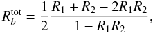
However, for γ = 0, only ox and oy are visible and orthogonal. Thus, in this case, we can identify σ+ and σ− with two indepenently absorbing media, i.e., light absorbed by σ+ does not affect σ−, and vice versa. This can be illustrated by two equal boxes, which can be filled with different absorbing materials of amounts m1 and m2, having however an identical central wavelength and line broadening. The boxes are evenly illuminated by a plane-parallel light source of total intensity Ic, while the emerging light is gathered at a detector with no spatial resolution (Fig. 2). For a plane-parallel atmosphere perpendicular to the LOS and containing only oscillators ox and oy, the content of the box 1 represents the amount of σ+ absorbers, and the content of the other box that of σ−. An empty box implies an absence of oscillators in that direction.
First, let the box 1 contain either m1 or
m2 amount of absorbers while the box 2 remain empty (this
most simple case is not illustrated in the figure). Then the corresponding observed
spectra  are obviously given by
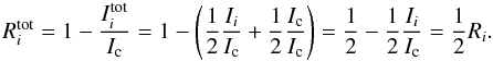
So, we observe exactly half the amount of the absorption as compared to the profiles Ii/Ic that would emerge directly from the box 1, because we also observe Ic passing through the other, empty box.
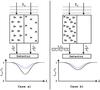 |
Fig. 2 Incident plane-parallel light Ic (dotted lines) is passing through two boxes, that can be filled with (identical) absorbing material (trianges, squares) and is detected by a spectrometer. The observed spectrum is plotted as solid line at the bottom of each panel. Left panel: the total line profile is the sum of the two individual profiles caused by only material 1 (I1/Ic, dashed line) and 2 (I2/Ic, dot-dashed line), respectively. Right panel: if box 1 contains both absorbing materials, the residual depth is calculated using Eqs. (10), (11), and cannot exceed a value 0.5, since half of Ic always passes through box 2. Saturation effects are visible in the center of the line. |
Now, if the box 1 is filled with m1 absorbers and the box 2 with m2, further referred to as case a), the total residual absorption depth is simply the sum of the individual values (Fig. 2, left panel):
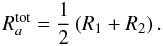
In the case b), the box 1 contains both m1 and m2 while the box 2 is again empty (Fig. 2, right panel). The contributing profiles form a total residual depth Rtot according to Eqs. (10) and (11), yielding
where for simplicity we assumed the saturation depths R0,i to be equal 1.
When we assume m1 + m2 of ox, such as in case b), the atmosphere is transparent for light with the electric field vector along ŷ. For an unpolarized light source Ic, this means that only half the amount of light will be subject to absorption, with the other half simply transmitted. In case a), our model atmosphere contained the same total amount of oscillators as in case b), but divided among ox, oy with multiplicity m1, m2. Absorption now takes place “independently” in two different media, resulting in a different residual depth, as seen in Eqs. (17), (16).
The above experiment shows that it is essential to distinguish between the cases of combining components of the same type and of different types. Explicit formulae for calculating the total residual depth as function of γ and the three components will be given in Sect. 5.
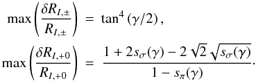
4.2. Anomalous splitting versus triplet approximation
So far we assumed that all spectral lines are Zeeman triplets, i.e., a transition splits into three magnetic components in the presence of a magnetic field. This is true for transitions J: 0 → 1, where J is the total angular momentum quantum number, and this case is called normal Zeeman effect. More often, for J > 1, transitions consist of multiple Zeeman subcomponents, and this case is called anomalous Zeeman effect. In principle, the latter can be approximated by the triplet case when the energy shifts within one kind of Zeeman components are replaced by a corresponding center of gravity. Here we assess the difference in Stokes profiles arising due to the triplet approximation as compared to the true transition splitting taking into account blending of the Zeeman subcomponents. We show that substantial errors can be made even for field strengths ≲1kG, depending on the line splitting. Therefore we further require our ZCD technique to be able to handle arbitrary Zeeman patterns, where we assume that the subcomponent profiles of each line are equal (hypothesis of complete redistribution, e.g. Landi Degl’Innocenti1976).
We will proceed by recalling the anomalous Zeeman effect and deriving an analytical expression for the location of the maximum Stokes V as a function of splitting and the line broadening parameter a in the case of a Voigt profile. Knowing the location of the maximum, we then compare the Stokes V amplitudes in the triplet and anomalous cases at this position for three different Zeeman patterns.
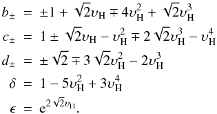
In the case of the anomalous Zeeman effect, the (2J + 1)-fold degenerate energy levels in the presence of a magnetic field split onto magnetic sublevels corresponding to M = −J,...,J. The selection rules (conditions for which the overlap integral does not vanish) require ΔJ = 0, ± 1, where J:0 → 0 is forbidden, and ΔM = 0, ± 1. For a given transition, the ensembles of subtransitions with ΔM = ∓ 1 are denoted as σ±, while those with ΔM = 0 are referred to as π0. In the Zeeman regime, both the splitting pattern and the individual strengths Sn of the subcomponents are symmetric around the central wavelength and depend on ΔJ and M as well as on the electron spin and orbital momentum (see, e.g., for atoms Sobelman1972; and for molecules Berdyugina & Solanki2002). In this case, the usual renormalization for the strengths Sn within each ΔM subset is

A mean energy shift of the σ-components is characterized by the effective Landé factor geff, i.e., the mean splitting weighted with the corresponding strengths. This is a way to describe arbitrary splittings in terms of a normal triplet. In the Paschen-Back regime, the symmetry around the central wavelength vanishes, and the sums of strengths for each ΔM are no longer equal (e.g., Berdyugina et al.2005). Here the line profile can be approximated by a triplet with the three different Landé factors g+, g0, and g−. Also, the violation of the selection rule ΔJ = 0, ± 1 has to be taken into account.
In stellar spectropolarimetry it is common to assume that the maximum Stokes V amplitude of a spectral line increases linearly with the product of the line of sight magnetic field component and geff of the line (WFA). Here we evaluate when this assumption loses its validity due to noticeable splitting. We partially adopt the notation of Stenflo (1994). For the magnetic quantum numbers Ml, Mu and the Landé factors gl, gu of the upper and lower levels, respectively, the individual Zeeman shifts for q = 1 (Ml = Mu + 1,andMn = Mu) are given by

with ωL = eB/2me the Larmor frequency, and the anomalous splitting in units of the Doppler broadening
To investigate the
deviations from the anomalous to the normal Zeeman effect, let us assume here that the
line profile is given by a Voigt function
H(a,υ) with
a = Γ/4πΔνD,
and a line central depth dc, instead of our unconstrained
profile  , yielding
In Eq. (21), we made use of the symmetry of the splitting pattern for the σ components. Note that we use dc in contrast to the usual definition using the line-to-continuum opacity ratio η. For the Zeeman triplet case (Eq. (1)), we define in accordance with Eq. (20) the Zeeman splitting in units of the Doppler broadening
To be able to assess the difference between multiplet splitting and the triplet approximation in terms of maximum amplitude in circular polarization, we need to know where Stokes V has its maximum. For weak magnetic fields and weak lines, V ∝ ∂H/∂υ (Stenflo1994), i.e., the location υmax where its derivative is largest is constant for υH ≪ 1. For a = 0, H is a Gaussian, and
We then approximate the dependence on the parameter a for B ≪ 1 by a linear function

From numerical simulations for various 0 < a ≤ 0.1 we find ma = 0.2855 ± 0.0003 (Fig. 3, left panel). Our calculated points show a constant offset of ~6.4 × 10⁻³, which does not influence the determination of ma.
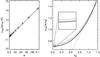 |
Fig. 3 Behaviour of the location where Stokes V is the largest as a function of the Voigt profile parameter a and the σ-component shift υH in the Zeeman triplet. Left panel: diamonds show the maximum positions υmax numerically calculated for different values of a and very small B (υH → 0). A linear fit (solid line) is sufficient to describe the dependence of υmax on a. Right panel: dashed lines are numerical simulations of υmax(a,υH) for a = 10-3,10-2,10-1. The dotted line describes its asymptotic behaviour when the line is fully split. The bold solid line is an analytical solution given by Eq. (26) for a = 0. |

Since there is no
analytical solution to this equation, we make a Taylor expansion up to the second order in
υ around the point  ,
which yields
,
which yields
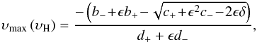
where
As shown in Fig. 3, the function given by Eq. (26) (bold solid line) is a good approximation for υH ≲1. For a magnetic field of ≲1kG, we have υH < 0.5, and the curves for a ≠ 0 (dashed lines) differ from that of a = 0 by a constant shift (cf. right panel scale-up) given by Eq. (24). Thus, combining these two equations, we finally obtain
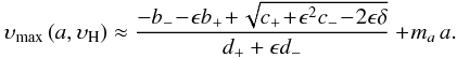
Using Eq. (28), we can now investigate the Stokes
V amplitude in the anomalous splitting case at the position where the
corresponding triplet approximation curve has its maximum. We consider three different
splitting patterns as shown on the left panel of Fig. 4. The relative errors δV/V
for these patterns as a function of (triplet) component shifts are shown in on the right
panel of Fig. 4. In cases where the sublevel
splitting is small
(Δυn ≪ υH,
e.g., in the transition  ),
the center of gravity approximation works very well (dashed curve). The intermediate case
matches the results from Semel et al. (2009).
However, if
Δυn ≲ υH, the
error increases rapidly with υH, reaching 10% (e.g., in
),
the center of gravity approximation works very well (dashed curve). The intermediate case
matches the results from Semel et al. (2009).
However, if
Δυn ≲ υH, the
error increases rapidly with υH, reaching 10% (e.g., in
 )
already at υH ~ 0.3. For example, a line with
λ0 = 6000Å, ΔλD = 0.1Å, and
geff = 2, will reach this value at
)
already at υH ~ 0.3. For example, a line with
λ0 = 6000Å, ΔλD = 0.1Å, and
geff = 2, will reach this value at
Since ΔλD ∝ λ, all curves in Fig. 4 scale with λ for a given Doppler velocity, rendering the triplet approximation worse at longer wavelengths. Note that δV/V depends on the the relative shifts and strengths of individual σ-components within a splitting pattern, and not on the absolute shift of the gravity center. The effect is therefore independent of geff.
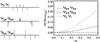 |
Fig. 4 Left panel: different types of anomalous Zeeman splitting patterns. The lengths and shifts of the bars from the center are proportional to the relative strengths and energy shifts, respectively. From Sobelman (1972). Right panel: deviation of the maximum Stokes V amplitude in the anomalous case with respect to that in the triplet approximation as a function of the triplet splitting in Doppler units. |
5. Explicit formulae
In this section we aim to provide analytic expressions for Stokes I,
Q, U, and V as functions of the three
common Zeeman profiles σ±, and π0.
The shape of each corresponds to the observable profile at B = 0 with an
average line depth of all contributing lines, and not to the underlying
intrinsic profile apprearing the Unno-Rachkovsky solutions (cf. the use of
dc in Eq. (21)). Similar to the line adding algorithm derived in Sect. 3, we will now explicitly see how different Zeeman components add up. In
other words, we will be able to write each Stokes parameter in terms of the three Zeeman
profiles, which differ only by a proportionality factor depending on central depths of the
contributing lines. So,  is our set of free parameters. Provided
has to be a list of wavelengths and quantum numbers of possible spectral lines for the input
spectrum. To keep the expressions at a comprehensive level, we skip the magnetooptical
effect throughout this section, for which the calculations work similarly.
is our set of free parameters. Provided
has to be a list of wavelengths and quantum numbers of possible spectral lines for the input
spectrum. To keep the expressions at a comprehensive level, we skip the magnetooptical
effect throughout this section, for which the calculations work similarly.
This offers us a valuable tool to disentangle the individual σ±, and π0 profiles of a (blended) line and to demonstrate the difference between blending of σ+ with σ− and of σ± with π0 components. Also, we can compare the result with that of linear models and emphasize the difficulties arising when the LSD or PCA combine Stokes profiles.
First, in Sect. 5.1 we show how the Zeeman component opacities can be expressed in terms of σ±, π0, γ and χ. Then, we substitute them into the radiative transfer solutions and obtain final expressions for Stokes I, Q, U, and V in Sect. 5.2 without a detailed discussion. Finally, in Sect. 5.3, we illustrate in detail the behaviour of Stokes I when two Zeeman component profiles are added up and discuss errors for a linear model.
5.1. Zeeman component opacities
The analytic radiative transfer solutions
RI,
RQ,
RU,
RV are functions of γ,
χ, and the local line opacities in units of the continuum opacity
η+ ,0, −, i.e.,
 . Explicit
expressions are provided by, e.g., Stenflo (1971),
and Arena et al. (1990). To express the Zeeman
component profiles via opacities, we first consider σ+ in
the longitudinal case, i.e., when the electron in the classical picture oscillates in the
x − y-plane perpendicular to the LOS. As shown in
Sect. 4.1, σ+ then
represents exactly half of the absorption capability of the medium. Therefore we have,
using Eq. (6)
. Explicit
expressions are provided by, e.g., Stenflo (1971),
and Arena et al. (1990). To express the Zeeman
component profiles via opacities, we first consider σ+ in
the longitudinal case, i.e., when the electron in the classical picture oscillates in the
x − y-plane perpendicular to the LOS. As shown in
Sect. 4.1, σ+ then
represents exactly half of the absorption capability of the medium. Therefore we have,
using Eq. (6)
when assuming R0 to be equal to 1.
To account for arbitrary orientations, we characterize the circular motion with frequency ω of the σ+ electron component by two linear oscillators, σx,σy:

If we incline the plane of oscillations of σ+ by the angle γ around the x-axis, the observed motion of σ+ becomes

The absorption efficiency
is equal to the squared time-average amplitude. If we also note that the observable motion
of the π-electron is proportional to sinγ, we get the
orientation factors  for the σ and π components, respectively:
![\begin{equation} \label{eq:orientfac1} s_{\sigma}\!\left(\gamma\right) = \frac{\omega}{2\pi} \int_0^{2\pi/\omega}\left[\cos\left(\omega t\right) + \sin\left(\omega t\right)\cos\gamma\right]^2 = 1\!-\!{\rm \frac{1}{2}}\sin^2\gamma, \end{equation}](/articles/aa/full_html/2010/14/aa14971-10/aa14971-10-eq177.png)
Using Eqs. (33) and (34), we obtain
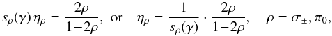
which simplifies to Eq. (30) for the σ components in the case of γ = 0.
Another way to see this is to insert, for instance, σ+ into RI of the Unno-Rachkovsky equations, and to solve the result for η+:
which after some algebra turns out to be equivalent to Eq. (35).
5.2. Final expressions for Stokes IQUV
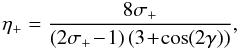
Knowing now the expressions for η+, η0 and η− in terms of the Zeeman component profiles σ+, π0, σ−, γ and χ, we can insert them into the transfer equation solutions and obtain the final expressions for Stokes parameters. In the general case, all three components contribute to the line profile:
![$$R_I\left(\sigma_+,\pi_0,\sigma_-,\gamma\right) = 1 + c_1 \left[1\!-\!\sigma_+\!-\!\pi_0\!-\!\sigma_-\!+\!4\sigma_+\pi_0\sigma_-\right]/\Delta$$](/articles/aa/full_html/2010/14/aa14971-10/aa14971-10-eq184.png)
![$$R_Q\left(\sigma_+,\pi_0,\sigma_-,\gamma,\chi\right) = s_{\sigma}\!\left(\gamma\right) \cos\left(2\chi\right)\Sigma / \left[2\Delta\right]$$](/articles/aa/full_html/2010/14/aa14971-10/aa14971-10-eq185.png)
![\begin{equation} \label{eq:fullIQUV} R_U\left(\sigma_+,\pi_0,\sigma_-,\gamma,\chi\right) = s_{\sigma}\!\left(\gamma\right) \sin\left(2\chi\right)\Sigma / \left[2\Delta\right] \end{equation}](/articles/aa/full_html/2010/14/aa14971-10/aa14971-10-eq186.png)

where
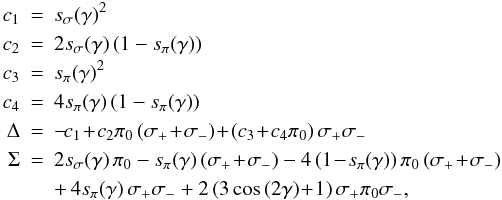
and
with  ,
,
 as given
in Eqs. (34).
as given
in Eqs. (34).
5.3. Combining two Zeeman components for Stokes I
In this section we discuss in detail how two arbitrary Zeeman component profiles blend together in Stokes I within our model. More specifically, we consider two pairs: σ+ and σ−, and σ+ and π0. Further, we derive and discuss expressions for errors arising when the components are added linearly.
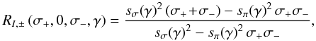
Since Stokes I does not depend on χ, we set this angle equal to 0 for the moment. From the radiative transfer solutions given by Eqs. (37), we obtain for the pair of the σ+ and σ− profiles:
and for the pair of the σ+ and π0 profiles:
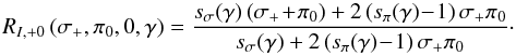
Figure 5 contains six panels, three rows of 2 panels each. In the follwing we refer to the three rows of panels in Fig. 5 as top, middle and lower panels (note that the middle panels share the abscissa values with the lower panels).
The two functions given by Eqs. (39) and (40) are plotted in the top panels of Fig. 5 for γ = π/4,3π/8,7π/16,15π/32,π/2 (solid lines, from top to bottom). For simplicity, we plot RI, ± and RI, + 0 assuming that in the first case σ+ = σ− and in the second case σ+ = π0. The result of the linear summation of the components is shown by dashed line. For small values of γ (< π/4), deviations from the linear case are small for both RI, ± and RI, + 0. However, combining σ± components for π/4 < γ ≲ π/2 results in noticeably smaller total depths, for all σ± ≤ 0.5. Note that the two special cases γ = 0 and γ = π/2 correspond to the left and right panels of Fig. 2, respectively.
To find the values of σ± and π0 for which the relative error introduced by the linear approximation is largest, we solve for σ+(= σ−)
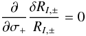
and an analogous equation for σ+(= π0), yielding
and
The middle panels of Fig. 5 show the functions given by Eqs. (42) and (43), respectively. For a pair of σ± components, the relative error at small γ is largest for intermediate component depths (σ± = 0.25), whereas for larger γ, the error is largest for stronger components. The relative error for RI, + 0 is always largest for 0.25 ≤ σ+(= π0) < 0.3, i.e., when σ- and π-profiles are of similar strengths in the Zeeman triplet.
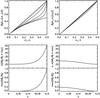 |
Fig. 5 Behaviour of RI, ± (σ+ + σ−, left panels), and RI, + 0 (σ+ + π0, right panels). Top panels: the resulting blend depth when both components have equal depth (abscissa values) for different angles γ ranging from π/4 to π/2 (top to bottom solid lines). The dashed line represents the linear sum of the two components. Middle panels: component depth for which the relative error with respect to the linear approximation δRI/RI is largest, depending on the angle γ. Lower panels: maximum relative errors δRI/RI as a function of γ. See text for detailed discussion. |
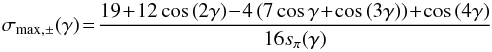
The values of the maximum errors are given by
Obviously, these occur at σmax, ± and σmax, + 0, respectively. The two functions are shown in the lower panels of Fig. 5. For RI, ± , the relative error is small for small γ, reaching 3% at γ = π/4, but it increases rapidly up to 100% for γ → π/2. When adding up σ+ and π0, the relative error is largest (~17%) for γ near 0 and decreases for larger inclination angles.
6. Numerical implementation
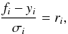
The ZCD algorithm is realized as an inversion procedure with the minimization of the discrepancy between the data y and the model f. Representing our set of Eqs. (34) for each pixel i in terms of the measurements yi with individual errors σi by
we search for the
solution which minimizes  by applying a Gauss-Newton
minimization method, as described by Sennhauser et al.
(2009). In contrast to other codes, instead of using response functions we find the
matrix of derivatives analytically for our parameters
BMOD,γ,χ,dc,Z,
which takes ~5 times the computing time of one evaluation step of the
function fi.
by applying a Gauss-Newton
minimization method, as described by Sennhauser et al.
(2009). In contrast to other codes, instead of using response functions we find the
matrix of derivatives analytically for our parameters
BMOD,γ,χ,dc,Z,
which takes ~5 times the computing time of one evaluation step of the
function fi.
For the evaluation of fi at wavelength
λi for the Zeeman subcomponent
k of the transition q
(q = −1,0,1) of the contributing line
j, we perform spline interpolation of our common line profile
 at the
velocity vijqk, whereas for the Jacobi matrix,
we use quadratic inverse interpolation.
at the
velocity vijqk, whereas for the Jacobi matrix,
we use quadratic inverse interpolation.
There exists an ambiquity between the amplitude of Z and the line depths
parameters dc. For example, consider that the spectral line
j has a “true” central depression of 0.5 at its laboratory wavelength
center λ0,j. Let ξ be the
current solution to the current linearized residual equations and
Z(v = 0) = 1, and
dc,j = 0.4 be the current parameter guesses.
Many variations
ξZ0,ξdc,j
of these two parameters may satisfy the condition
Z0·dc,j = 0.5.
Since we require the amplitude of Z to be equal to 1 during each step of
inversion, while the location of the maximum may well vary with respect to the initial
guess, we try to inflict any undesired amplitude change ΔZ as additional
alteration Δdc,j on the current
ξdc,j for all
lines j. Thus, assuming that  is a good solution, we look for a Δdc which satisfies the
condition
is a good solution, we look for a Δdc which satisfies the
condition
where
-
 , the
amplitude of the trial
Z' = Z + ξZ
located at
, the
amplitude of the trial
Z' = Z + ξZ
located at  ;
; -
 , the value of
the current Z at the location where Z' is
max;
, the value of
the current Z at the location where Z' is
max; -
ΔZ = A' − 1, the difference in overall amplitude (the amplitude of the current Z equals 1).
Rearranging Eq. (46) we find
If the current Z and dc were good parameters already, Eq. (46) simplifies to
and
The new parameters will then be
where normalization by A' ensures the new amplitude to be equal to 1.
7. Application to simulated data
Here we demonstrate the performance of the ZCD method using simulated data. The input spectra have to be normalized to the continuum, which is the only requirement (ordering or spectral interval between pixels is not required). We first apply it to Stokes I,V data and explore its capability to recover a longitudinal magnetic field BLOS from circular polarization signals fully embedded in noise (Sect. 7.1). Then, we employ another set of I,Q,U,V simulated data, allowing us to retrieve the full magnetic field vector (Sect. 7.2). We compare the inferred common line profiles (and the corresponding mean Stokes V profiles) with those obtained by the LSD technique with and without deblending (see Sennhauser et al.2009).
We have simulated a local solar-type spectrum (temperature, element abundance) using the full polarized radiative transfer code STOPRO (see Sect. 3.1) for references with a variety of noise levels and magnetic field vectors, convolved with Gaussian to account for instrumental broadening. The spectrum includes 35 atomic lines in the wavelength interval between 521.5 and 529.8nm, and all of them are used to retrieve unknown parameters. However, for better visibility, we show in the figures only 15 lines in the window from 526.2 to 526.65nm in the figures. Note that the line central depths parameters were assumed to be altogether unknown. The spectral resolution of the simulated spectra was of ~30 mÅper pixel, i.e. typical for high-resolution solar spectropolarimetry. The chosen binsize for the ZCD common Zeeman profile was 1.14km s-1.
7.1. Longitudinal magnetic fields: Stokes I, V
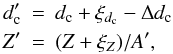
To test the capability of the ZCD to retrieve only BLOS, Stokes I,V data with B = 20G and γ = 0, and a continuum noise of 1% were generated. These are shown in Fig. 6 with dotted lines in the upper two panels. Best fits obtained with the ZCD are drawn with solid lines. For comparison, the noise-free input spectrum for Stokes V is shown as dash-dotted line. It hardly deviates from the ZCD fitted spectrum. The lower left panel shows the inferred common Stokes I profile from our ZCD method (solid line) corresponding to the recovered BLOS = 18 G. The common profiles from the LSD with deblending (dashed) and the standard LSD (dash-dotted) are superposed. Note that in order to compare them to the ZCD, they had to be renormalized.
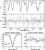 |
Fig. 6 The result of the ZCD deployed to Stokes I,V simulated data. Upper panels: simulated (dotted) and recovered (solid line) spectra for Stokes I and V, as well as the noise-free input spectrum (dash-dotted line) for Stokes V. Lower panels: retrieved common line profiles from the ZCD (solid) and from the LSD with/without deblending (dashed/dash-dotted lines) for Stokes I (left panel) and V (right panel). |
The striking difference between the common line profiles obtained with the LSD and our ZCD method is a substantial broadening of the former. This is because of the following two reasons: first, line strengths influence the shape of the LSD profile, as stronger lines are broader than optically thin lines, while the ZCD profile is not affected by the strengths of the contributing lines. Secondly, contributions from blends, which are either not accounted, as in the standard LSD, or improperly (linearly) added, as in the deblending LSD, cause a noticeable broadening, especially in the far wings of the profile (see dash-dotted curve at v ~ 10 km s-1 in Fig. 6, lower left panel).
For a comparison, we also created a common Stokes V profile from the ZCD common line profile, using averaged line parameters, as in other multi-line techniques. The lower right panel of Fig. 6 shows the obtained circular polarization signatures. Clearly, the noise is too high for the LSD to recover a reasonable signal from the Stokes V only (dashed and dash-dotted lines). For the ZCD, applied to the Stokes I and V simultaneously, the Zeeman component profiles are well constrained by the intesity spectrum. This allows for a much more precise determination of the component separation and results in a resonable average Stokes V profile.
We further tested the reliability of our ZCD method by varying an imposed noise. We produced 125 simulated spectra with the same BLOS of 20 G for each noise level between 1/6% and 1%. Figure 7 shows the recovered BLOS for two sets of 25 spectra with the noise levels of 0.33% (stars) and 1% (triangles). The average magnetic field strength values of 20.1 ± 3.2G (stars) and 18.4 ± 9.1G (triangles) are close to the true value of 20 G. The same is valid for other noise levels: 19.9G, 19.8G, 20.4G, 19.7G, 20.0G, while the uncertainty increases proportionally to the SNR of the input spectra (Fig. 7, lower panel). We also varied initial magnetic field strength values Binit between −50 and 50 G to demonstrate the independence of the solution on the initial guess. We conclude that for this spectrum, the ZCD is robust up to the noise level a factor of ~5 larger than the mean Stokes V amplitude. This gain can be further increased by employing a larger number of spectral lines.
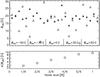 |
Fig. 7 Top panel: retrieved magnetic field strengths obtained by the ZCD deployed to 20G Stokes I,V data with the noise levels of 0.33% (stars) and 1% (triangles). The results are shown for two sets of 25 spectra with different initial values for BLOS. Lower panel: standard deviations of BLOS from 125 runs each at different noise levels. |
7.2. Inclined magnetic fields: Stokes IQUV
To test the capability of the ZCD to deal with full Stokes data, we simulated spectra with BMOD = 200G, γ = 70°, and χ = 30°. Figure 8 shows results obtained from the ZCD when 0.2% noise is added to the spectra. The top four panels display the data (dotted) and the fits (solid lines) for Stokes I, V, Q, and U, as well as the noise-free input spectra (dash-dotted lines) for Stokes QUV. The lower left panel shows the inferred ZCD common Zeeman profile (solid line), as well as the retrieved magnetic field parameters. The corresponding profiles obtained using the LSD with (dashed) and without deblending (dash-dotted) are plotted too. The Stokes I profiles reveal the same issues for the LSD profiles as in the case of a longitudinal field (Sect. 7.1). But with a circular polarization signal-to-noise ~7 times higher in this case than in the previous one, the LSD also detects a reasonable Stokes V signature (lower right panel).
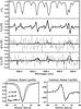 |
Fig. 8 The result of the ZCD deployed to Stokes IQUV simulated data. Top four panels: simulated (dotted) and fitted (solid line) spectra for Stokes I, V, Q, and U, as well as the noise-free input spectra (dash-dotted lines) for Stokes QUV. Lower panels: retrieved common line profiles from the ZCD (solid), and from the LSD with/without deblending (dashed/dash-dotted lines) for Stokes I (left panel) and V (right panel). |
The ZCD is also capable of extracting meaningful linear polarization signals despite the high noise level (S/N < 1) and to determine the orientation of the magnetic field. While the fit from ZCD for Stokes V coincides with the noise-free input spectrum, Stokes Q and U show the limitations of Eqs. (37). The remaining low noise ripples in the fitted linear polarization spectra in Fig. 8 are due to the fact that our Zeeman component profile is not constrained to be neither symmetric nor monotonic in the wings.
We have again tested the robustness of the ZCD solution by adding different amounts of noise to the same spectrum and simulating 100 different realizations for each noise level. The results are shown in Fig. 9, where three panels present expectation values with error bars for the magnetic field parameters BMOD, γ and χ.
The best-fit parameters BMOD and γ showed
distributions close to normal, and we calculated their expectation values as the means for
each noise level. The distribution of χ values showed however three
peaks, i.e. far from a normal distribution. The highest peak was at 30°, the
second one at 60°, and a (smaller) third one at 150°. The
explanation for this is as follows. As can be seen in Eqs. (3), Stokes Q and U have a (different)
trigonometric dependence on χ. Only determination of
Q/U selects the correct values for
χ. Therefore, if the noise distribution allows the code to identify
both Stokes Q and U signals, the ratio is well defined,
and χ is found correctly (within a normal distribution). However, if
Stokes Q is too much embedded in noise (which is more probable than for
U for our choice of χ), the code picks one of two
equally probable angles:  or 60°. If
Q is detectable but U is not, then it finds
or 60°. If
Q is detectable but U is not, then it finds
 or 150°.
We attempted to account for this special kind of distribution and considered values of 60° and 150° as partially true. We applied the following formula for the expectation value of χ

where
 denote
the mean value. The lowest panel of Fig. 9 shows these weighted mean values
⟩χ⟨. One can see that they are
within 10% of the true value for all tested noise levels, whereas the standard deviations
are all larger than 10%, reaching 100% for the 0.5% noise.
denote
the mean value. The lowest panel of Fig. 9 shows these weighted mean values
⟩χ⟨. One can see that they are
within 10% of the true value for all tested noise levels, whereas the standard deviations
are all larger than 10%, reaching 100% for the 0.5% noise.
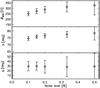 |
Fig. 9 Statistical analysis of the results from the ZCD deployed to full Stokes spectra with (BMOD = 200G, γ = 70°, χ = 30°). Expectation values and standard deviations for the magnetic field parameters were obtained from 100 runs at each noise level. |
For BMOD and γ there is a clear trend to increase for higher noise levels. However, the LOS component of the field is quite stable. In addition, the functions for the mean recovered values saturate for high noise levels, not exceeding 350G and 80°, respectively. We explain this behaviour as follows. The inversion procedure has two ways of fitting stochastic features created by the noise in the linear polarization spectra: by increasing BMOD and/or γ. Since our considerable Stokes V signal constrains in first order only the LOS component of B, both BMOD and γ increase. This effect saturates chiefly because of the constraints by Stokes I (line broadening, or splitting, respectively).
8. Conclusions
We have developed an efficient method, the Zeeman component decomposition, which is able to extract a common Zeeman component profile from high-resolution broad-band Stokes I,Q,U,V spectra. The shape of this profile is fully unconstrained. This makes the ZCD useful for studying stellar (and solar) inhomogenous atmospheres. We consider that all Stokes parameters comprise this common profile, assuming that each line forms locally in a Milne-Eddington atmosphere. Being based on the analytical radiative transfer solutions, the ZCD overcomes limitations of the weak-field and weak-line approximations, which are typical for other multi-line techniques.
The advantage of the ZCD is that it is applied simultaneously to all Stokes parameters, assuming a uniform magnetic field. The intensity spectrum strongly contrains the profile, while polarized spectra provide essential information on the magnetic vector. In other words, we allocate the z + n + 3 (common profile + n lines + magnetic vector) free parameters to the individual Stokes parameters according to their information content (with the magnetic parameters allocated to all of them with different weights). The signal-to-noise ratio for Stokes I is normally two orders of magnitude larger than for Stokes V, which in turn is ~10 times larger than for Q and U. Therefore, Stokes I defines the common profile and line central depths, with only BMOD, γ and χ being left for the polarized spectra. BMOD is responsible for the individual shifts of the component profiles, while γ and χ basically determine the ratios of Q, U and V. Other multi-line techniques applied to individual Stokes spectra operate with 4 × z free parameters, relying on the precise a priori knowledge of line central depths, so that the interpretability of 3 × z of them is questionable and strongly affected by noise. From this point of view the advantage of the ZCD can be easily seen. Thus, solving for the Zeeman component profile we obtain at the same time parameters of the full magnetic field vector in the line forming region. We showed that the ZCD is capable to retrieve reliable values from very challenging, i.e., noisy spectra. Furthermore, the fact that the recovered line central depths on average deviate by no more than 0.024 from the predetermined values strongly reduces the dependency on knowledge of stellar parameters. The only fixed parameters left are the two intrinsic transition parameters energy shift (wavelength), and electronic configuration.
In this paper, we presented and illustrated with examples main principles of the ZCD. While not constraining the common line profile allows for diverse atmospheric conditions, the inferred magnetic field strength and orientation are assumed to be uniform. Further improvements can be done to account for strong rotational and/or instrumental broadening. These posterior convolution effects on spectra are known to degrade the functionality of deconvolution techniques, because the process of line formation and convolution with a non-delta kernel are noncommuting mathematical operations. A solution to this problem shall be discussed in a forthcoming paper.
At the same time, we will further develop ZCD into a code for Zeeman Doppler imaging. In contrast to existing methods, our approach shall dynamically assess the number of resolution elements necessary to reproduce the observations, expanding the overall profile into a series of local sub-profiles. We shall thereby overcome the limitation of a uniform magnetic field to model arbitrary polarization profiles, even from single snapshots. Despite the spatial mapping inherent to every Doppler imaging technique, this approach should maintain the high sensitivity to very weak magnetic fields, as well as the ability to model strong magnetic fields, of the current ZCD method.
In the Paschen-Back regime, individual strengths of the Zeeman components are different. Knowing the relative values of the strengths (e.g., Landi Degl’Innocenti & Landolfi2004; Berdyugina et al.2005) helps to rescale the components.
Acknowledgments
We thank the referee, Prof. G. A. Wade, for many valuable comments that helped improve the paper. This work is supported by the EURYI (European Young Investigator) Award provided by the European Science Foundation (see http://www.esf.org/euryi) and SNF grant PE002-104552.
References
- Arena, P., Landi Degl’Innocenti, E., & Noci, G. 1990, 129, 259 [Google Scholar]
- Berdyugina, S. V., & Solanki, S. K. 2002, 385, 701 [Google Scholar]
- Berdyugina, S. V., Solanki, S. K., & Frutiger, C. 2003, 412, 513 [Google Scholar]
- Berdyugina, S. V., Braun, P. A., Fluri, D. M., & Solanki, S. K. 2005, 444, 947 [Google Scholar]
- Donati, J.-F., Semel, M., Carter, B. D., Rees, D. E., & Cameron, A. C. 1997, 291, 658 [Google Scholar]
- Frutiger, C., Solanki, S. K., Fligge, M., & Bruls, J. H. M. J. 2000, 358, 1109 [Google Scholar]
- Landi Degl’Innocenti, E. 1976, 25, 379 [Google Scholar]
- Landi Degl’Innocenti, E., & Landolfi, M. 2004, Polarization in Spectral Lines (Dordrecht: Kluwer) [Google Scholar]
- Lites, B. W., Kubo, M., Socas-Navarro, H., et al. 2008, 672, 1237 [Google Scholar]
- Martínez Gonzáles, M. J., Asensio Ramos, A., Carroll, T. A., et al. 2008, 486, 637 [Google Scholar]
- Mihalas, D. 1978, Stellar atmospheres (San Francisco: W. H. Freeman and Company) [Google Scholar]
- Orozco Suárez, D., Bellot Rubio, L. R., del Toro Iniesta, J. C., et al. 2007, 670, 61 [Google Scholar]
- Rachkovsky, D. N. 1962a, 27, 148 [Google Scholar]
- Rachkovsky, D. N. 1962b, 28, 259 [Google Scholar]
- Ruiz Cobo, B., & del Toro Iniesta, J. C. 1992, 398, 375 [Google Scholar]
- Semel, M. 1989, 225, 456 [Google Scholar]
- Semel, M., & Li, J. 1996, Sol.Phys., 164, 417 [Google Scholar]
- Semel, M., Ramírez Vélez, J. C., Martínez González, M. J., et al. 2009, 504, 1003 [Google Scholar]
- Sennhauser, C., Berdyugina, S. V., & Fluri, D. M. 2009, 507, 1711 [Google Scholar]
- Sobelman, I. I. 1972, Introduction to the Theory of Atomic Spectra (Braunschweig: Pergamon Press) [Google Scholar]
- Solanki, S. K. 1987, Ph.D. Thesis, ETH, Zurich, Switzerland [Google Scholar]
- Stenflo, J. O. 1971, IAUS, 43, 101 [Google Scholar]
- Stenflo, J. O. 1994, Solar Magnetic Fields (Dordrecht: Kluwer) [Google Scholar]
- Unno, W. 1956, PASJ, 8, 108 [NASA ADS] [Google Scholar]
All Figures
|
Fig. 1 Behaviour of a given line Rλ (thick line) with a varying strength. The scaling function fλ is given by Eq. (14). |
| In the text | |
|
Fig. 2 Incident plane-parallel light Ic (dotted lines) is passing through two boxes, that can be filled with (identical) absorbing material (trianges, squares) and is detected by a spectrometer. The observed spectrum is plotted as solid line at the bottom of each panel. Left panel: the total line profile is the sum of the two individual profiles caused by only material 1 (I1/Ic, dashed line) and 2 (I2/Ic, dot-dashed line), respectively. Right panel: if box 1 contains both absorbing materials, the residual depth is calculated using Eqs. (10), (11), and cannot exceed a value 0.5, since half of Ic always passes through box 2. Saturation effects are visible in the center of the line. |
| In the text | |
|
Fig. 3 Behaviour of the location where Stokes V is the largest as a function of the Voigt profile parameter a and the σ-component shift υH in the Zeeman triplet. Left panel: diamonds show the maximum positions υmax numerically calculated for different values of a and very small B (υH → 0). A linear fit (solid line) is sufficient to describe the dependence of υmax on a. Right panel: dashed lines are numerical simulations of υmax(a,υH) for a = 10-3,10-2,10-1. The dotted line describes its asymptotic behaviour when the line is fully split. The bold solid line is an analytical solution given by Eq. (26) for a = 0. |
| In the text | |
|
Fig. 4 Left panel: different types of anomalous Zeeman splitting patterns. The lengths and shifts of the bars from the center are proportional to the relative strengths and energy shifts, respectively. From Sobelman (1972). Right panel: deviation of the maximum Stokes V amplitude in the anomalous case with respect to that in the triplet approximation as a function of the triplet splitting in Doppler units. |
| In the text | |
|
Fig. 5 Behaviour of RI, ± (σ+ + σ−, left panels), and RI, + 0 (σ+ + π0, right panels). Top panels: the resulting blend depth when both components have equal depth (abscissa values) for different angles γ ranging from π/4 to π/2 (top to bottom solid lines). The dashed line represents the linear sum of the two components. Middle panels: component depth for which the relative error with respect to the linear approximation δRI/RI is largest, depending on the angle γ. Lower panels: maximum relative errors δRI/RI as a function of γ. See text for detailed discussion. |
| In the text | |
|
Fig. 6 The result of the ZCD deployed to Stokes I,V simulated data. Upper panels: simulated (dotted) and recovered (solid line) spectra for Stokes I and V, as well as the noise-free input spectrum (dash-dotted line) for Stokes V. Lower panels: retrieved common line profiles from the ZCD (solid) and from the LSD with/without deblending (dashed/dash-dotted lines) for Stokes I (left panel) and V (right panel). |
| In the text | |
|
Fig. 7 Top panel: retrieved magnetic field strengths obtained by the ZCD deployed to 20G Stokes I,V data with the noise levels of 0.33% (stars) and 1% (triangles). The results are shown for two sets of 25 spectra with different initial values for BLOS. Lower panel: standard deviations of BLOS from 125 runs each at different noise levels. |
| In the text | |
|
Fig. 8 The result of the ZCD deployed to Stokes IQUV simulated data. Top four panels: simulated (dotted) and fitted (solid line) spectra for Stokes I, V, Q, and U, as well as the noise-free input spectra (dash-dotted lines) for Stokes QUV. Lower panels: retrieved common line profiles from the ZCD (solid), and from the LSD with/without deblending (dashed/dash-dotted lines) for Stokes I (left panel) and V (right panel). |
| In the text | |
|
Fig. 9 Statistical analysis of the results from the ZCD deployed to full Stokes spectra with (BMOD = 200G, γ = 70°, χ = 30°). Expectation values and standard deviations for the magnetic field parameters were obtained from 100 runs at each noise level. |
| In the text | |
Current usage metrics show cumulative count of Article Views (full-text article views including HTML views, PDF and ePub downloads, according to the available data) and Abstracts Views on Vision4Press platform.
Data correspond to usage on the plateform after 2015. The current usage metrics is available 48-96 hours after online publication and is updated daily on week days.
Initial download of the metrics may take a while.