| Issue |
A&A
Volume 522, November 2010
|
|
|---|---|---|
| Article Number | A79 | |
| Number of page(s) | 12 | |
| Section | Catalogs and data | |
| DOI | https://doi.org/10.1051/0004-6361/201014870 | |
| Published online | 04 November 2010 | |
A spectroscopic survey of faint, high-Galactic-latitude red clump stars
I. The high resolution sample
1
INAF-OAPD – Osservatorio Astronomico di Padova,
via dell’Osservatorio 8,
36012
Asiago (VI),
Italy
e-mail: marica.valentini@oapd.inaf.it, valentini@astro.ulg.ac.be
2
Dipartimento di Astronomia, Universitá di Padova,
vicolo dell’Osservatorio 3,
35122
Padova,
Italy
e-mail: ulisse.munari@oapd.inaf.it
3
Institut d’Astrophysique et de Géophysique de l’Université de
Liège, Allée du 6 Août
17, 4000
Liège,
Belgium
Received:
27
April
2010
Accepted:
31
May
2010
Context. Their high intrinsic brightness and small dispersion in absolute magnitude make red clump (RC) stars a prime tracer of Galactic structure and kinematics.
Aims. We aim to derive accurate, multi-epoch radial velocities and atmospheric parameters (Teff, log g, [M/H], Vrotsini) of a large sample of carefully selected RC stars, fainter than those present in other spectroscopic surveys and located over a great circle at high Galactic latitudes.
Methods. We acquired data of the program stars of high signal-to-noise ratio (S/N) and high resolution with the Asiago Echelle spectrograph. Radial velocities were obtained by applying cross-correlation and atmospheric parameters via χ2 fit to a synthetic spectral library. Extensive tests were carried out by re-observing with the same instrument a large number of standard stars taken from a variety of sources in the literature. During these tests, we found that the absolute Tycho VT magnitude of local red clump stars is not dependent on metallicity
Results. A total of 277 red clump stars (101 of them with a second epoch observation) of the extended solar neighborhood and 55 calibration stars were observed and included in an output catalog that contains (in addition to relevant support astrometric and photometric data taken from literature) the main output of our survey: accurate multi-epoch radial velocities (σ(RV)⊙ ≤ 0.4 km s-1), accurate atmospheric parameters (σ(Teff) = 68 K, σ(log g) = 0.11 dex, σ([M/H]) = 0.10 dex, σ(Vrotsini) = 1.1 km s-1), distances, and space velocities (U,V,W).
Key words: Galaxy: kinematics and dynamics / Galaxy: structure / solar neighborhood
© ESO, 2010
1. Introduction
Since the pioneering work of Cannon (1970) and Faulkner & Cannon (1973), the clump on the red giant branch of open clusters has been recognized as having been formed by stars in the stage of central helium burning. These authors interpreted the near constancy of the clump absolute magnitude as the result of He ignition in an electron-degenerate core. Under these conditions, He burning cannot begin until the stellar core mass attains a critical value of about 0.45 M⊙. It then follows that low-mass stars developing a degenerate He core after H exhaustion, have similar core masses at the beginning of He burning, and hence a similar luminosity, as discussed in detail by Girardi et al. (1999). A great contribution to the study of red clump stars (hereafter RC stars) came from the availability of Hipparcos parallaxes (Perryman et al. 1997). On the CMD of nearby stars built from precise Hipparcos parallaxes, the red clump is a prominent and well populated feature. The Hipparcos catalog (ESA 1997) contained ~600 RC stars with a parallax error σπ/π ≤ 10% (Girardi et al. 1998), a wealth of data that made it possible to transform the RC stars into calibrated standard candles.
Several calibrations of the absolute magnitude of RC stars have been carried out. Keenan & Barnbaum (1999) found the absolute magnitude of the RC stars in the optical to range from MV = +0.70 for those of spectral type G8 III to MV = +1.00 for the K2 III ones. From a sample of 228 RC stars (satisfying the selection conditions σπ/π ≤ 10%, +0.8 ≤ V − I ≤ +1.25, and −1.4 ≤ MI ≤ +1.2 mag), Paczynsky & Stanek (1998) found MI = −0.28 ± 0.09, with no significant dependence on metallicity. Adopting the same selection criteria for a larger sample of ~600 RC stars observed by Hipparcos et al. (1998) obtained MI = −0.23 ± 0.03 and confirmed the absence of any dependence on metallicity. Udalski (2000), using the same selection conditions as Paczynsky & Stanek (1998), found instead a weak dependence on metallicity in the form MI = −0.26(±0.02) + (0.13 ± 0.07)([Fe/H] + 0.25). Alves (2000) found MK = −1.61 ± 0.03, with a negligible dependence on metallicity in the form MK = −1.64(±0.07) + (0.57 ± 0.36)([Fe/H] + 0.25). Groenewegen (2008), working this time with the revised Hipparcos parallaxes of van Leeuwen (2007), found slightly fainter absolute magnitudes for RC stars, MI = −0.22(±0.03), and MK = −1.54(±0.04), confirming a null or very weak dependence on metallicity. These calibrations imply that the absolute magnitude of the red clump of the solar neighborhood has a rather small (or null) dependence on metallicity. However, Sarajedini (1999) and Twarog et al. (1999), working on open clusters, found some dependence of the absolute magnitude of RC on metallicity and age, which is supported by the theoretical models of stellar populations by Girardi & Salaris (2001), and Salaris & Girardi (2002).
RC stars have been used to derive the distance, among others, to the Galactic center (Paczynsky & Stanek 1998), Fornax (Rizzi et al. 2007), M33 (Kim et al. 2002), and LMC (Salaris et al. 2003), and to isolate components of the Galaxy, such as the central bar of the Galaxy and the Canis Major accreted dwarf galaxy, or determine gradients along the Sagittarius stream (Stanek et al. 1997; Bellazzini et al. 2006a,b; Rattenbury et al. 2007).
A number of investigations have focused on the atmospheric properties and/or radial velocities of bright and nearby RC stars. McWilliam (1990) compiled an extensive catalog of 671 G-K giants, mostly RC giants, for which he derived Teff from broad-band photometry, log g via isochrone fitting (which was carried out by invoking heterogeneous calibrations of the absolute magnitude), and individual chemical abundances by means of an LTE analysis of high resolution spectra, while no radial velocity was measured. Mishenina et al. (2006) derived both the radial velocity and the atmospheric parameters for 177 RC stars. Values of Teff, [M/H] and elemental abundances were derived from the classic line-by-line spectroscopic analysis (imposing excitation and ionization equilibrium on selected FeI and FeII lines), while log g was determined by combining the ionization balance of iron and fitting the wings of the CaI 6162.17 Å line. Atmospheric parameters without radial velocities were obtained by Hekker & Melendez (2007) and Takeda et al. (2008). They studied 366 G- and K-type giants and 322 intermediate-mass late-G giants, respectively, with many RC stars among them, by adopting the classic line-by-line method based on FeI and FeII lines recorded in high resolution spectra. Finally, Famaey et al. (2005) carried out a survey of giant stars with CORAVEL, deriving precise radial velocities for all the K stars with MHip < 2 and M stars with MHip < 4 mag present in the Hipparcos catalog. Their survey provides radial velocities, but not the atmospheric parameters, for a sample of ~6600 K giants, mostly RC stars.
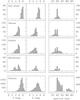 |
Fig. 1 Distribution of V, K and spectral type of the red clump stars in our survey and the surveys of Takeda et al. (2008), Hekker & Melendez (2007), Mishenina et al. (2006), and Famaey et al. (2005). |
2. Motivation for this survey
The afore mentioned, high-resolution spectroscopic surveys of RC stars generally focused only on atmospheric parameters or radial velocities, but not on both simultaneously, with the exception of the 177 RC stars observed by Mishenina et al. (2006). They were also limited to the brighter RC stars in the solar neighborhood, as illustrated in Fig. 1 by the distribution in V and K magnitude of their target stars. In addition, they typically observed the target stars only once, so that binaries (identified on the basis of varying radial velocities) could not be recognized and internal errors could not be consistently evaluated by comparing of the results of different reobservations. To improve upon some of these shortcomings, we conceived a new, extensive and multi-epoch high resolution spectroscopic survey of RC stars, to which we refer in this paper as the Asiago Red Clump spectroscopic Survey (ARCS). This paper introduces the survey and its data output, while a companion paper (Valentini et al. 2010, in prep.) explores some first science results of the survey, and yet another paper in the series (Saguner & Munari 2010, in prep.) will extend the survey to even fainter magnitudes.
The ARCS survey observes a sample of carefully selected genuine RC stars, distributed along the great circle of the celestial equator, away from the Galactic plane and the effects of its extinction, fainter by ≥ 2 mag (and consequently more distant) than the surveys of Mishenina et al. (2006), Hekker & Melendez (2007), and Takeda et al. (2008), and ~1 mag fainter than Famaey et al. (2005). The magnitude distribution of the ARCS targets is presented in Fig. 1. An original feature of the ARCS survey, is the derivation of the atmospheric parameters by χ2 fitting an extensive library of synthetic spectra (that of Munari et al. 2005, the same adopted by the RAVE survey). The χ2 approach is the method of choice for massive spectroscopic surveys such as the ongoing RAVE project with the 6dF fiber positioner at the UK Schmidt telescope in Australia, the soon-to-be launched Gaia, the ESA’s successor to Hipparcos, and the all-sky survey to be carried out with LAMOST (Xinglong, China). The first two surveys focus on a limited wavelength range centered on the far-red CaII triplet, RAVE observing at a resolving power 7500 and Gaia planned for 11 500. ARCS, observing at twice that resolving power (20 000) and over a much wider and bluer wavelength range (4800–5900 Å), provides an useful term of comparison to evaluate the performances and elaborate on possible improvements. In addition, ARCS reobservation at a second epoch (spaced in time by at least one month) of 1/3 of the program stars, provided that an accurate estimate has been made of the contamination to radial velocities by binarity or pulsations, and of the repeatibility of derived atmospheric parameters.
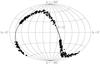 |
Fig. 2 Aitoff projection in Galactic coordinates of our program stars. The thick line is the celestial equator. |
3. Target selection criteria
The targets selected for ARCS had to meet stringent criteria designed to provide a clean sample of genuine, unreddened RC stars, easily observable from the northern latitudes of the Asiago observatory, and supported by accurate spectroscopic classification and Hipparcos/Tycho-2 proper motions.
The first enforced selection criteria concerned the spectral type of the target stars and their position on the sky. Essentially all RC stars present in the Hipparcos catalog have spectral types between G8III and K2III. We thus looked at the most complete and homogeneous set of spectroscopic classifications, the Michigan Project. It covers the HD stars of the whole southern sky up to +6° northern declination (Houk & Swift 2000). From the Michigan Project catalog, we selected giants from spectral types G8III to K2III satisfying the conditions: (i) high accuracy of the spectral classification (quality index ≤ 2 and blank duplicity index in the Michigan catalog); (ii) a declination within 6° of the celestial equator (to facilitate observations from Asiago and to confine the targets to a great circle on the sky); and (iii) a Galactic latitude |b| ≥ 25° (to avoid reddening close to the plane of the Galaxy).
We then turned to astrometric and photometric selection criteria. The ARCS targets must also (iv) be valid entries in both the Hipparcos1 and Tycho-2 catalogs; (v) possess non-negative Hipparcos parallaxes; and (vi) avoid any other Hipparcos or Tycho-2 star closer than 10 arcsec on the sky. Furthermore, the target stars must (vii) be confined within the magnitude range 6.8 ≤ VTycho − 2 ≤ 8.1 (to be fainter than targets in other spectroscopic surveys of RC stars, and at the same time still preserving meaningful Hipparcos parallaxes); and (viii) have an absolute magnitude (from Hipparcos parallax) incompatible with either luminosity classes V or I. The targets must also (ix) have a blank photometric variability flag and a blank duplicity index in the Hipparcos catalog (to the aim of rejecting stars affected by binarity and/or pulsations); and (x) be present in the 2MASS survey (so that their optical-IR spectral energy distribution could be derived in combination with BT and VT from Tycho-2, and (V − I)C from the Hipparcos catalog).
Finally, we looked at overlaps with other spectroscopic surveys. We (xi) rejected stars already present in the Nördstrom et al. (2004) Geneva-Copenhagen survey of dwarfs in the solar neighborhood, or included in the radial velocity survey of giant stars by Famaey et al. (2005). This set of eleven selection criteria provided a total of 381 target stars for ARCS, from which those actually observed were randomly selected according to the local sideral time at the telescope. By the end of the observing campaign, we had observed 207 ARCS targets, 66 of which (1/3 of the total) had been observed at two distinct epochs.
Wavelength range of the Echelle orders used in our analysis.
Additional RC stars, brighter than the target set, were observed for calibration purposes, to ensure commonality with other surveys, and tests. A total of additional 70 RC stars, with spectral type between G8III and K2III, were observed with an instrument set-up identical to that for ARCS targets, and for 35 of them (half of the total) a distinct second epoch observation was in addition collected. These calibration RC stars are discussed in detail later in the paper, where the tests on the accuracy of radial velocities and atmospheric parameters are described. Of the calibration RC stars, 10 were selected from Takeda et al. (2008), 10 from Hekker & Melendez (2007), 12 from Soubiran et al. (2005), 3 from Mishenina et al. (2006), and 4 are members of the Praesepe open cluster.
Finally, a sample of an additional 55 non-RC stars were observed, primarly for calibration purposes. They include 16 well-know field stars, 24 stars from the RAVE survey (Zwitter et al. 2008), 2 stars from Soubiran et al. (2005), 9 members of Coma Berenices, and 4 members of Praesepe open clusters.
4. Data acquisition and reduction
The target stars were observed with the REOSC Echelle spectrograph and CCD mounted at Cassegrain focus of the Asiago 1.82m telescope. The recorded spectra cover the wavelength range from 3700 to 7300 Å in 30 orders. To maximize S/N and avoid the redder wavelength region contaminated by telluric absorptions, the data analysis was limited to the 9 adjacent echelle orders covering the wavelength range from 4815 to 5965 Å, from Hβ to NaI doublet (cf Table 1).
Being detectable only redward of 6350 Å, fringing was not an issue. Throughout the whole observing campaign, the slit orientation was kept fixed to east-west and its width on the sky to 1.9 arcsec, which corresponds to a resolving power of 20 000. The spectra were obtained as three separate and consecutive exposures, each lasting 4 min. Before reduction, the three individual frames were median combined into a single one to automatically reject cosmic rays and increase the S/N. The three exposures were autoguided to increase the sharpness in the spatial direction of the recorded spectrum. Along the dispersion axis, the parameters of the autoguider were set to allow the stellar image to move for an amount equivalent to half of the slit width, to achieve a more uniform illumination of the entire slit width and consequently minimize any radial velocity offset (see next section).
The spectra were reduced and calibrated with IRAF, using standard dark, bias and dome flats calibration exposures. Special care was devoted to the 2D modeling and subtraction of the scattered light. Deep exposures of moonlight scattered by the night sky were also obtained and later cross-correlated to the calibrated stellar spectra. No cross-correlation peak was found other than that expected from the stellar spectrum. In particular, higher velocity stars did not display a secondary peak close to zero velocity. These results confirmed that the sky subtraction procedure accurately removed, from the extracted stellar spectra, the scattered moonlight. Therefore, any possible residual moonlight was strong enough to neither contaminate the measurement of radial velocities, nor the determination of atmospheric parameters.
Exposures of a thorium lamp for wavelength calibration were obtained both immediately before and soon after the three exposures of the star, on which the telescope was still tracking. These two exposures of the thorium lamp were combined before extraction, to compensate for spectrograph flexures. From the start of the first thorium exposure to the end of the last, the whole observing cycle on a program star took about 15 min. According to the detailed investigation and 2D modeling by Munari and Lattanzi (1992) of the flexure pattern of the REOSC echelle spectrograph mounted at the Asiago 1.82 m telescope, and considering that we preferentially observed our targets when they were crossing the meridian, the impact of spectrograph flexures on our observations corresponds to an uncertainty smaller than 0.1 km s-1, thus completely negligible. This is fully confirmed by (1) the measurement by cross-correlation of the radial velocity of the rich telluric absorption spectrum in the red portion of all our spectra, and (2) the measurement of all night sky lines we detected in our spectra, relative to the compilations of their wavelengths by Meinel et al. (1968), Osterbrock & Martel (1992), and Osterbrock et al. (1996).
Given both the red colors of the RC stars and the instrument response, the S/N of recorded spectra was found to steeply increase with increasing wavelength. Over the 9 adjacent echelle orders considered for the measurement of the radial velocity and derivation of the atmospheric parameters, the S/N per pixel was – for all target stars – generally higher than 50 for the bluest order and higher than 120 for the reddest one.
5. Radial velocities
The radial velocity of the program stars was obtained by cross-correlating (cf. Tonry & Davis 1979) with the synthetic spectral library of Munari et al. (2005), in its version matching the 20 000 resolving power of our echelle spectra.
5.1. Continuum normalization
In both the determination of radial velocities via cross-correlation and atmospheric parameters via χ2 fitting, the echelle spectra had to be accurately continuum normalized. The procedure of continuum normalization that we adopted had three steps.
All spectra were first manually normalized, one by one, order by order. The normalization blaze functions of each order proved to be fairly constant, and by averaging them together, we obtained a mean normalization function for each individual order. The second step consisted of applying the mean normalizations to the orders of all spectra. The resulting normalized spectra were individually inspected and compared with each other to identify low spatial frequency deviations of the continua from linear slopes, and – if required – a second normalization pass was manually carried out. The third and final step was to automatically renormalize, with exactly the same parameters, both the synthetic spectra and the observed spectra, as preliminarily normalized by the two steps just described. We selected the synthetic spectra in their continuum normalized form, cutting out the wavelength intervals matching those of the nine echelle orders selected for science operations. The adopted function for automatic renormalization was a Legendre polynomial of 6th order with high reject of 1.5 and low reject of 0.5.
The adopted procedure accurately placed the observed spectra onto exactly the same normalization system as the synthetic spectra, improving the accuracy of the χ2 fitting, for which the most important factor was the S/N of the observed spectra.
5.2. Velocity measurement
The radial velocity was derived separately for each of the 9 echelle orders selected for science applications. The 9 different measurements almost always agreed to within 0.6 km s-1, so that the internal error in the mean was smaller than 0.2 km s-1. The very few cases in which the error exceeds the 0.6 km s-1 spread, were found to be related to specific problems with a single echelle order, which was therefore ignored when deriving the final velocity for that spectrum and in the subsequent atmospheric analysis.
The zeropoint of the wavelength (and therefore velocity) scale was checked for each spectrum by cross-correlating the telluric O2 and H2O absorption spectra recorded in various echelle orders external to the 9 selected for science applications. In particular, the B (centered on ~6900) and A (~7620 Å) absorption systems by O2, and a (~7200) by H2O were used. The illumination of the slit aperture by telluric absorptions is obviously identical to that of the stellar seeing disk, and thus traces all wavelength conversion effects more accurately than the use of night-sky emission lines that instead illuminate uniformly the whole slit width. In the vast majority of cases, the resulting radial velocity of O2 and H2O telluric absorption systems was smaller than ±0.25 km s-1, and no correction was applied to the stellar radial velocity. In a few cases, the shift for O2 and H2O lines was larger than ±0.25 km s-1, and the radial velocity of the corresponding stellar spectrum was corrected for. This invariably occurred with observations characterized by particularly good seeing, when the FWHM of the stellar image was appreciably smaller than the projected slit width.
5.3. Multi-epoch observations, binaries, pulsations
As previously noted, 66 RC stars belonging to the target list and 35 of the calibration set were reobserved at a second epoch. Comparison of the radial velocities at the two distinct epochs provides both (i) an evaluation of the internal accuracy of the radial velocities, as well as (ii) a means of isolating binaries or stars affected by pulsations.
Figure 3 shows the histogram of the differences in radial velocity between the two epoch observations of the 101 reobserved program stars. The vast majority belong to a sharp distribution characterized by a median difference of 1.2 km s-1, indicating that binarity and pulsations are not a significant concern for the bulk of the RC stars selected for ARCS. The median value 1.2 km s-1 is at least twice as large as the combined internal errors, and to it some contribution must be provided by wide and low mass ratio binaries, or low amplitude pulsations.
Ten stars are distinctive in Fig. 3 for large differences in radial velocity of the two epoch observations. The difference is far larger than the observational errors, and consequently these stars are regarded as candidate binaries or affected by large amplitude pulsations (radial modes). We have initiated additional observations of these ten stars to help identify the cause of the radial velocity variability. The results of these will be reported elsewhere.
5.4. Accuracy tests on IAU standards
With the same instrument set-up and data reduction adopted for ARCS, we observed 7 RC stars that are also IAU standard radial velocity stars (Table 2). The mean difference between ours and literature values is ΔRV⊙= −0.13 km s-1, with an rms of 0.3 km s-1. This confirms both the absence of a zeropoint offset in the system of ARCS radial velocities based on cross-correlation against appropriate synthetic template spectra, as well as their high external accuracy.
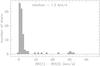 |
Fig. 3 Distribution of the difference in velocity between two observations ( ≥ one month apart) for 101 program stars. |
Comparison with tabular values of the radial velocity we derived for seven RC stars that are also IAU standard RV stars.
5.5. Accuracy tests on RAVE stars
A sample of 24 stars, well distributed in terms of luminosity class among those of spectral types F, G, and K, were randomly selected from the RAVE second data release (Zwitter et al. 2008) among those most easily observable from Asiago.
We observed them with the same instrument set-up and data reduction adopted for ARCS. Table 3 compares the RAVE radial velocities with ours. The mean difference between ours and RAVE velocities is ΔRV⊙ = +0.4 km s-1, with an rms of 1.1 km s-1, if we ignore the first two stars in Table 3 (one a rapidly rotating early F star, the other an M star with emission-line cores). Again, the comparison provides reassurance about the quality of ARCS radial velocities, considering in particoular that the mean accuracy of radial velocities reported in the RAVE second data release is ±1.5 km s-1.
6. Atmospheric parameters
The same continuum normalized spectra prepared for the measurement of radial velocities were used in the derivation of the atmospheric parameters Teff, log g, [M/H], and Vrotsini via χ2 fitting to the synthetic spectral library of Munari et al. (2005), which is based on the atmospheric models by Castelli & Kurucz (2003). The same synthetic library is adopted (in its version at resolving power 7500) for the atmospheric analysis by the RAVE Survey (Steinmetz et al. 2006; Zwitter et al. 2008).
To hasten the convergence of the χ2 fitting, we considered only the version of the synthetic library for [α/Fe] = 0.0. Thus the metallicity we derived refers to all metals, and is not divided into that of the iron-peak elements separated and that of the α elements. A development we are pursuing for the ARCS survey is the derivation of individual chemical abundances using a classical line-by-line approach, which will be presented in a future paper, and that will naturally address the α-enhancement. The Munari et al. (2005) library adopts an homogeneous micro-turbulence velocity of ξ = 2 km s-1, which is appropriate for RC stars (as proven by the high resolution studies of Hekker & Melendez 2007; Takeda et al. 2008; Soubiran et al. 2005).
6.1. Repeated observations
Comparing the χ2 for the nine different Echelle orders, we obtained an rms in the single spectrum of 47 K in Teff, 0.21 dex in log g, 0.10 dex in [M/H], and 1 km s-1 in Vrotsini.
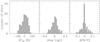 |
Fig. 4 Differences in temperature, gravity, and metallicity between reobservations of 101 program stars. |
As discussed in Sect. 5.3, we obtained distinct observations of 101 RC stars at two epochs separated by at least one month. Figure 4 presents the distributions of the differences in Teff, log g, and [M/H] between these two observations. The distributions are quite sharp, well centered on 0.0 and characterized by σ(Teff) = 39 K, σ(log g) = 0.24, and σ([M/H] ) = 0.04.
6.2. Comparison with literature data on red clump stars
Hekker & Melendez (2007), Soubiran et al. (2005), and Takeda et al. (2008) provide atmospheric parameters for many RC stars based on the classical line-by-line method of imposing excitation and ionization equilibrium on a selected sample of FeI and FeII lines.
We reobserved with exactly the same procedures and instrumental set-up adopted for ARCS stars, a total of 10 RC stars from the list of Hekker & Melendez (2007), another 10 RC stars from Takeda et al. (2008), and 8 RC stars from Soubiran et al. (2005). From the latter, we reobserved an additional four giants lying outside the G8III-K2III interval covered by ARCS targets, bringing the total to 32 objects in common. The results are presented in Table 4. Figure 5 shows the comparison for each echelle order individually. It exhibits no obvious dependence on the S/N of the recorded spectrum on the given order.
The mean differences between our results and those of Hekker & Melendez (2007) for the stars in common are ⟨ (Tour − THM) ⟩ = −45 K (σ = 76 K), ⟨ (log gour − log gHM) ⟩ = −0.05 dex (σ = 0.25), and ⟨ ([M/H]our − [M/H]HM) ⟩ = −0.26 dex (σ = 0.05). The comparison with Soubiran et al. (2005) yields ⟨ (Tour − TSou) ⟩ = +15 K (σ = 54 K), ⟨ (log gour − log gSou) ⟩ = +0.01 dex (σ = 0.12), and ⟨ ([M/H]our − [M/H]Sou) ⟩ = −0.12 dex (σ = 0.15). Finally the comparison with Takeda et al. (2008) gives ⟨ (Tour − TTak) ⟩ = +21 K (σ = 62 K), ⟨ (log gour − log gTak) ⟩ = +0.15 dex (σ = 0.32), and ⟨ ([M/H]our − [M/H]Tak) ⟩ = −0.27 dex (σ = 0.04).
We note that there are systematic differences between the sources in literature. For the 147 stars in common among them, Teff and log g from Takeda et al. (2008) are on average ~50 K cooler and ~0.25 dex lower, respectively, than those of Hekker & Melendez (2007), while no appreciable differences exist in terms of metallicity. These differences are very close to those we found, with Takeda et al. (2008) being 66 K cooler, 0.20 dex lighter, and the same metallicity as Hekker & Melendez (2007).
 |
Fig. 5 ΔTeff, Δlog g, and Δ[M/H] versus S/N for the nine Echelle orders. The plotted values are the differences with respect to the mean. Full circles are objects from Hekker & Melendez (2007), empty circles from Soubiran et al. (2005), and stars from Takeda et al. (2008). |
Combining the results of the comparison with Hekker & Melendez (2007), Takeda et al. (2008), and Soubiran et al. (2005), for the 32 RC stars in common, we found that


![\begin{eqnarray} \langle([M/H]_{\rm our}- [M/H]_{\rm lit})\rangle&=&-0.21 ~~\pm 0.03 ~~(\sigma=181). \end{eqnarray}](/articles/aa/full_html/2010/14/aa14870-10/aa14870-10-eq92.png)
The differences in Teff and log g are negligible, and even smaller than the errors of the mean. In contrast, the mean difference in metallicity is significant. It is similar in amount and arithmetic sign to the mean difference between the metallicity from literature and that derived by the RAVE survey (Zwitter et al. 2008, who also adopt a χ2 fitting approach).
To place our results on the same atmospheric scale as that of the RC stars in literature, we therefore added +0.21 to our metallicities and this corrected value is listed in the catalog associated with this data release, while no addition of an offset was required for temperatures and gravities.
Figure 6 plots the differences in Teff, log g, and [M/H] between our results and those of Hekker & Melendez (2007), Takeda et al. (2008), and Soubiran et al. (2005) for the 32 RC stars in common. Apart from the rigid shift in metallicity, Fig. 6 shows that there are no systematic trends.
6.3. Tests on open clusters
To check the external consistency of our atmospheric parameters measurements, we also observed a set of stars belonging to open clusters whose atmospheric parameters were retrieved from literature. This comparison confirms the results about the RC stars in the previous section.
We observed 9 members the Coma Berenices open cluster, with spectral types from F2III to G2V. The results are presented in Table 5 (available electronic only). The average difference in temperature is ⟨(TARCS − Tlit)⟩ = +12 K (σ = 200 K), and in metallicity ⟨([M/H]ARCS − [M/H]lit)⟩ = −0.26 dex (σ = 0.08).
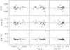 |
Fig. 6 Differences between atmospheric parameters obtained with our χ2 technique and literature values. Full circles are objects from Hekker & Melendez (1997), empty circles from Soubiran (2005), and stars from Takeda et al. (2008). Input data from Table 4. |
We also observed four RC stars in the Praesepe open cluster. The results are presented in Table 6 (available electronic only). The average difference in temperature is ⟨(TARCS − Tlit)⟩ = +13 K (σ = 200 K), and in metallicity ⟨([M/H]ARCS − [M/H]lit)⟩ = −0.24 dex (σ = 0.15).
Comparison between the atmospheric parameters of some members of the Coma Berenices open cluster (Mel 111) as given in literature and derived via χ2 fitting.
Comparison between the atmospheric parameters of some red clump members of the Praesepe open cluster (NGC 2632) as given in literature and derived via χ2 fitting.
6.4. Comparison with photometric temperatures
Temperatures derived from photometric indices are usually considered in atmospheric analysis. Most frequently, they are used as a starting point in the iterative analysis based on the ionization and excitation equilibrium of FeI and FeII lines from high resolution spectroscopy (e.g. Gratton et al. 2006; Fulbright et al. 2007), but sometimes they are directly imported as fixed values into abundance analysis (e.g. McWilliam 1990; Honda et al. 2004). The most frequently used color index for deriving photometric temperatures is V − K. Two of the most widely adopted calibrations of Teff as a function of V − K applicable to G-K giants (and therefore to RC stars), were presented by Ramirez & Melendez (2005) and McWilliam (1990).
Adopting the final corrected metallicity derived by our χ2 analysis, we computed the temperature of our program stars following Ramirez & Melendez (2005), who elaborated upon and expanded previous extensive work by Alonso et al (1996, 1999). The form of their relation is complex
![\begin{displaymath} T_{\rm eff}=5040/\theta_{\rm eff} + P\{(V-K),[{\rm Fe/H}]\}, \end{displaymath}](/articles/aa/full_html/2010/14/aa14870-10/aa14870-10-eq107.png)
where
![\begin{eqnarray} \theta_{\rm eff}&=&0.4813 + 0.2871(VK) - 0.0203(V-K)^2 \nonumber \\ & &-0.0045(V-K)[{\rm Fe/H}] + 0.0062[{\rm Fe/H}] \nonumber \\ & &- 0.0019[{\rm Fe/H}]^2, \nonumber \end{eqnarray}](/articles/aa/full_html/2010/14/aa14870-10/aa14870-10-eq108.png)
and P{(V − K),[Fe/H]} is a polynomial expression that takes different forms over different ranges of metallicity. Here the V band is VT Tycho-2, and K is the Ks from 2MASS. The comparison with our temperatures is shown in the top two, left panels of Fig. 7. The median difference is 88 K (photometric temperatures being cooler) and there is also a systematic trend, with photometric temperatures drifting progressively toward cooler values as the temperature inferred from χ2 increases.
The form of the relation between Teff and V − K proposed by McWilliams (1990) is simpler, and does not contain terms depending on metallicity, i.e., Teff = 8595 − 2349(V − K) + 321(V − K)2 −8(V − K)3, where V and K are standard Johnson bands. The comparison with our temperatures is shown in the top two right panels of Fig. 7. We obtained the Johnson V magnitudes from VT Tycho-2 following the transformation by Bessell (2000), while the K magnitudes were assumed to be equal to Ks from 2MASS without transformation. The median difference from our χ2 temperatures is much smaller, this time just 18 K (photometric temperatures being cooler), while the slope of the least squares fitting is only 15% steeper than in the case of Ramirez & Melendez (2005). The comparison between Teff derived following Ramirez & Melendez (2005) & McWilliam (1990) is given by the crosses in Fig. 8, and clearly illustrates the systematic offset of 70 K between the two calibrations.
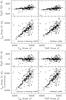 |
Fig. 7 Comparison between our temperatures and those derived from the (V − K) color calibrations of Ramirez & Melendez (2005, left column) and McWilliam (1990, right column). Top panels: using original Teff/(V − K) relations. The dashed line is the 1:1 relation, the thick solid line the least squares fit. Bottom panels: as above but with corrected Teff/(V − K) relations as explained in the text (Sect 6.4 and Eqs. (4) and (5)). |
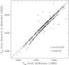 |
Fig. 8 Comparison between the Ramirez & Melendez (2005) and McWilliam (1990) Teff/(V − K) relations in their original form (crosses), and after the correction proposed in the text (open circles). |
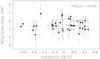 |
Fig. 9 Absolute magnitude in the Tycho VT band, as a function of metallicity, for the stars in the calibration set characterized by high Galactic latitude (b ≥ 25°), high astrometric accuracy (σ(π)/π ≤ 15 %, and low reddening (EB − V ≤ 0.1). |
For the sake of discussion, we searched for simple correction terms to the expressions of Ramirez & Melendez (2005) and McWilliams (1990) that would remove the differences between them and with χ2 temperatures. The correction terms are
![\begin{equation} T_{\rm Ram Mel}^{\rm corrected} = T_{\rm Ram Mel} - 255[(V-K) - 3.027] \end{equation}](/articles/aa/full_html/2010/14/aa14870-10/aa14870-10-eq119.png)
for Ramirez & Melendez (2005), and
![\begin{equation} T_{\rm McWilliam}^{\rm corrected} = T_{\rm McWilliam} - 305[(V-K) - 2.607] \end{equation}](/articles/aa/full_html/2010/14/aa14870-10/aa14870-10-eq120.png)
for McWilliam (1990). The relation between these corrected temperatures and our χ2 values is shown in the four bottom panels of Fig. 7. The corrections eliminate both the offsets and the trends. This of course reflects also the closer agreement between the Ramirez & Melendez (2005) and McWilliams (1990) temperatures, as illustrated by the open circles in Fig. 8.
That photometric temperatures are systematically cooler than spectroscopic ones is a well documented finding. Hill et al. (2000) found a mean difference of ΔTeff = 150 K, Allende Prieto et al. (2004) derived ΔTeff = 119 K, Mishenina et al. (2006) obtained ΔTeff = 47 K, Hekker & Melendez found ΔTeff = 56 K, and Takeda et al. (2008) got ΔTeff ~ 50 K. We note that Kovtyukh et al. (2006) found that photometric temperatures derived following Alonso et al. and Ramirez & Melendez formulations are 50 K cooler than spectroscopic ones, while the difference with McWilliam (1990) reduces to 19 K, very similar to our results.
The corrections to Eqs. (4) and (5) have a negligible effect on the dispersion of the points in Fig. 7, which remains high, with an rms of 195 K for both Ramirez & Melendez (2005) and McWilliams (1990). This is far larger than the rms of 61 K (and both null offset and null trend) in the difference between our χ2 temperatures and those of Hekker & Melendez (2007), Soubiran et al. (2005), and Takeda et al. (2008) for the 32 program stars in common discussed above. It confirms that while photometric temperatures may be useful starting points, a far more robust determination of Teff is obtained by either the FeI/FeII line-by-line analysis and the χ2 fitting.
The larger dispersion in the points in Fig. 7 toward hotter temperatures is caused by the Wien peak of the stellar energy distribution moving toward shorter wavelengths. When both bands are on the Rayleigh-Jeans tail of the energy distribution, the V − K color is less sensitive to Teff. The effective wavelength of the Tycho-2 VT band for the spectral type K0III is 5375 Å, and that of the Johnson V band is 5575 Å (cf. Fiorucci & Munari 2003). Thus, while for 4200 K the Wien peak at 6900 Å is still in-between the V and K bands, at 5200 K it matches the effective wavelength of the V band with a consequent rapid loss in sensitivity.
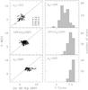 |
Fig. 10 Left columns present, for three different bins in the error of parallaxes and for all our program red clump stars, a comparison between the distance modulus obtained with the photometric parallaxes from Keenan & Barnbaum (2000) calibrations and distance modulus obtained with the revised Hipparcos parallaxes of van Leeuwen (2008). The lines represent the 1:1 correspondence. Each different spectral type is represented with a different symbol. The right columns give the corresponding distribution in VT magnitudes. |
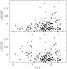 |
Fig. 11 Relation between orbital energy and surface gravity. The top panel is built assuming that all stars share the same luminosity class III, the bottom one assuming a luminosity class II for stars with log g ≤ 2. |
7. Absolute magnitudes and distances
As illustrated in Sect. 1, there is some controversy in the literature about whether the absolute magnitude of RC stars does or does not depend on metallicity. Figure 9 plots the Tycho-2 absolute magnitude M(VT) as a function of metallicity for the RC stars in our calibration set (thus matching the same selection criteria as our target RC stars, except for their brighter apparent magnitude) that have the most precise revised Hipparcos parallaxes (σ(π)/π ≤ 15 %) and lowest reddening (EB − V < 0.1). There is no statistically significant dependence on metallicity, and the mean absolute magnitude is ⟨ M(VT) ⟩ = +0.54.
Previous works on RC stars have been based on distances derived from Hipparcos parallaxes. This is a valid approach as long as the error in the astrometric parallax is small. This is not the case for our fainter target stars, for which the median error in the Hipparcos parallax is σ(π) / π ≥ 50%. The corresponding uncertainity is ≥ 50% in the distance, and ≥ 0.88 mag in the distance modulus (m − M).
We therefore decided to derive uniform spectrophotometric distances for all our program stars. We adopted the intrinsic absolute magnitudes in the Johnson V band calibrated by Keenan & Barnbaum (2000). They are given separately for the various spectral types (G8III to K2III) covered by our program stars, and are calibrated on RC stars with the most precise Hipparcos parallaxes. To derive the distances, we transformed the Tycho-2 VT into the corresponding Johnson V band following Bessell (2000) relations, and adopted the reddening derived from the all-sky mapping by Arenou et al. (1992). How these distances compare with the revised Hipparcos distances (van Leeuwen 2007) is illustrated in the left panels of Fig. 10. There, the various spectral types are plotted separately. For the RC stars with the most accurate revised Hipparcos parallaxes (σ(π)/π < 10%), there is no offset and the distances derived adopting Keenan & Barnbaum (2000) absolute magnitudes are aligned along the 1:1 relation. This proves the validity of our choice for the reference absolute magnitudes. For RC stars with revised Hipparcos parallaxes of intermediate precision (10% ≤ σ(π)/π ≤ 20%), the correspondence is still good even if the tail to the right in the distribution caused by the degraded astrometric parallaxes starts to become visible. Finally, for stars with a revised Hipparcos parallax of low accuracy (σ(π)/π > 20%), Fig. 10 clearly illustrates how spectrophotometric distances are more accurate and unbiased.
Content and description of the annexed catalog.
The energy of the Galactic orbit of a star should obviously be unrelated to its surface gravity (which is instead correlated with the absolute magnitude). To check this, we plot in the upper panel of Fig. 11 all our program RC stars in a log g/orbital energy diagram (for derivation of U, V, W component velocities see next section). Stars at 1 ≤ log g ≤ 2 have an orbital energy systematically lower than stars at log g ≥ 2. We note that the surface gravity of genuine RC stars is confined to log g ≥ 2, once our observational errors are properly take into account, while the surface gravity of G-K giants of luminosity class II is 1 ≤ log g ≤ 2 (cf. Straižys 1992). If the absolute magnitude of the 1 ≤ log g ≤ 2 stars in Fig. 11 is revised to that given by Sowell et al. (2007) for luminosity class II, the diagram in the lower panel of Fig. 11 is obtained. There the orbital energy of 1 ≤ log g ≤ 2 stars is equal to that of log g ≥ 2 stars, as it should be. Therefore, in the catalog associated with this paper, the distance (and related quantities) for these 26 1 ≤ log g ≤ 2 stars is listed as being derived assuming for them a luminosity class II and thus considering erroneous the luminosity class III listed in the Michigan Project Catalog V (Houk & Swift 2000). These 26 stars of luminosity class II are obviously not included in Fig. 10, which is meant to validate the absolute magnitudes of Keenan & Barnbaum (2000) for genuine RC stars (thus luminosity class III).
8. The catalog
The results of our survey is presented in the annexed catalog, available only in electronic form. Its format and content are illustrated in Table 7. In addition to the survey products, the catalog also includes photometric and astrometric information retrieved from the literature. Results from separate observational epochs are both listed. A conversion of the space velocity to the usual (U, V, W) system by using as input data position (α, δ), proper motion (μα, μδ), radial velocity, and distance was carried out following the formalism of Johnson & Soderblom (1987). We adopted a left-handed system with U becoming positive outwards from the Galactic center.
The catalog is divided into three main parts, reflecting the target selection criteria discussed in Sect. 3. It contains 433 entries, for 332 stars, 101 of them reobserved at a second epoch.
The first part of the catalog focuses on the target stars (those plotted in the brightness distribution histograms of Fig. 1), which are not present in other surveys of RC and giant stars. They are 207, and for 66 of them the results of a second observation are given.
The second part focuses on brighter RC stars, observed for both calibration purposes and to ensure commonality with other surveys of RC stars. There are 70 RC stars, and for half of them (35 stars), the catalog gives the results of a second epoch observation. In this second part of the catalog, we have first listed calibration RC stars (31 in all) not present in other survey and sharing (except for a brighter apparent magnitude) the same selection criteria as those for the objects included in the first part of the catalog (the target set). We have then listed the other calibration RC stars in common with other surveys (39 stars).
Finally, the third part of the catalog lists the results for all other 55 test and calibration stars that are not RC stars.
All selection criteria involving Hipparcos information refer to the original catalog published by ESA in 1997, and not necessarily its revision by van Leeuwen (2007).
Acknowledgments
We would like to thank R. Barbon for assistance during the realization of the project, K. Freeman for encouragement and useful advice, F. van Leeuwen for comments of revised Hipparcos distances, P. Valisa for assistance with the collection of some spectra, T. Saguner for useful discussions, and especially M. Fiorucci for coding part of the χ2 pipeline we adopted. This work has been in part supported by grant PRIN INAF 2008 (P.I. Michele Bellazzini, INAF-OABO).
References
- Alves, D. R. 2000, ApJ, 539, 732 [NASA ADS] [CrossRef] [MathSciNet] [Google Scholar]
- Alonso, A., Arribas, S., & Martinez-Roger, C. 1996, A&A, 313, 873 [NASA ADS] [Google Scholar]
- Alonso, A., Arribas, S., & Martinez-Roger, C. 1999, A&AS, 140, 261 [NASA ADS] [CrossRef] [EDP Sciences] [Google Scholar]
- Arenou, F., Grenon, M., & Gomez, A. 1992, A&A, 258, 104 [NASA ADS] [Google Scholar]
- Bellazzini, M., Newberg, H. J., Correnti, M., Ferraro, F. R., & Monaco, L. 2006a, A&A, 457, L21 [NASA ADS] [CrossRef] [EDP Sciences] [Google Scholar]
- Bellazzini, M., Ibata, R., Martin, N., et al. 2006b, MNRAS, 366, 865 [NASA ADS] [Google Scholar]
- Bessell, M. S. 2000, PASP, 112, 961 [NASA ADS] [CrossRef] [Google Scholar]
- Boesgaard, A. M. 1987, ApJ, 321, 967 [NASA ADS] [CrossRef] [Google Scholar]
- Boesgaard, A. M. 1989, ApJ, 336, 798 [NASA ADS] [CrossRef] [Google Scholar]
- Cannon, R. D. 1970, MNRAS, 150, 111 [NASA ADS] [CrossRef] [Google Scholar]
- Castelli, F., & Kurucz, R. L. 2003, Modelling of Stellar Atmospheres, 210, 20P [Google Scholar]
- Cayrel, R., Cayrel de Strobel, G., & Campbell, B. 1988, The Impact of Very High S/N Spectroscopy on Stellar Physics, 132, 449 [Google Scholar]
- Cayrel de Strobel, G. 1990, MemSAIt, 61, 613 [Google Scholar]
- Cayrel de Strobel, G., Soubiran, C., & Ralite, N. 2001, A&A, 373, 159 [NASA ADS] [CrossRef] [EDP Sciences] [Google Scholar]
- Claria, J. J., Piatti, A. E., & Osborn, W. 1996, PASP, 108, 672 [NASA ADS] [CrossRef] [Google Scholar]
- ESA 1997, Proceedings of the ESA Symposium Hipparcos – Venice ’97, ESA SP, 402 [Google Scholar]
- Famaey, B., Jorissen, A., Luri, X., et al. 2005, A&A, 430, 165 [NASA ADS] [CrossRef] [EDP Sciences] [Google Scholar]
- Faulkner, D. J., & Cannon, R. D. 1973, ApJ, 180, 435 [NASA ADS] [CrossRef] [Google Scholar]
- Fiorucci, M., & Munari, U. 2003, A&A 401, 781 [NASA ADS] [CrossRef] [EDP Sciences] [Google Scholar]
- Friel, E. D., & Boesgaard, A. M. 1992, ApJ, 387, 170 [NASA ADS] [CrossRef] [Google Scholar]
- Fulbright, J.P., McWilliam, A., & Rich, R.M. 2007, ApJ 661, 1152 [Google Scholar]
- Gebran, M., Monier, R., & Richard, O. 2008, A&A, 479, 189 [NASA ADS] [CrossRef] [EDP Sciences] [Google Scholar]
- Girardi, L. 1999, MNRAS, 308, 818 [NASA ADS] [CrossRef] [MathSciNet] [Google Scholar]
- Girardi, L., & Salaris, M. 2001, MNRAS, 323, 109 [NASA ADS] [CrossRef] [Google Scholar]
- Girardi, L., Groenewegen, M. A. T., Weiss, A., & Salaris, M. 1998, MNRAS, 301, 149 [NASA ADS] [CrossRef] [Google Scholar]
- Gratton, R., Bragaglia, A., Carretta, E., & Tosi, M. 2006, ApJ 642, 462 [NASA ADS] [CrossRef] [Google Scholar]
- Groenewegen, M. A. T. 2008, A&A, 488, 935 [NASA ADS] [CrossRef] [EDP Sciences] [Google Scholar]
- Gustafsson, B., Kjaergaard, P., & Andersen, S. 1974, A&A, 34, 99 [NASA ADS] [Google Scholar]
- Hekker, S., & Meléndez, J. 2007, A&A, 475, 1003 [NASA ADS] [CrossRef] [EDP Sciences] [Google Scholar]
- Honda, S., Aoki, W., Kajino, T., et al. 2004, ApJ, 607, 474 [NASA ADS] [CrossRef] [Google Scholar]
- Houk, N., & Swift, C. 2000, VizieR Online Data Catalog, 3214, [Google Scholar]
- Johnson, D. R. H., & Soderblom, D. R. 1987, AJ, 93, 864 [NASA ADS] [CrossRef] [Google Scholar]
- Keenan, P. C., & Barnbaum, C. 1999, ApJ, 518, 859 [NASA ADS] [CrossRef] [Google Scholar]
- Kim, M., Kim, E., Lee, M. G., Sarajedini, A., & Geisler, D. 2002, AJ, 123, 244 [NASA ADS] [CrossRef] [Google Scholar]
- McWilliam, A. 1990, ApJS, 74, 1075 [NASA ADS] [CrossRef] [Google Scholar]
- Meinel, A. B., Aveni, A. F., & Stockton, M. W. 1968, Tucson, Optical Sciences Center and Steward Observatory, University of Arizona. [Google Scholar]
- Mishenina, T. V., Bienaymé, O., Gorbaneva, T. I., et al. 2006, A&A, 456, 1109 [NASA ADS] [CrossRef] [EDP Sciences] [Google Scholar]
- Munari, U., & Lattanzi, M. G. 1992, PASP, 104, 121 [NASA ADS] [CrossRef] [Google Scholar]
- Munari, U., Sordo, R., Castelli, F., & Zwitter, T. 2005, A&A, 442, 1127 [NASA ADS] [CrossRef] [EDP Sciences] [Google Scholar]
- Nordström, B., Mayor, M., Andersen, J., et al. 2004, A&A, 418, 989 [NASA ADS] [CrossRef] [EDP Sciences] [Google Scholar]
- Osterbrock, D. E., & Martel, A. 1992, PASP, 104, 76 [NASA ADS] [CrossRef] [Google Scholar]
- Osterbrock, D. E., Fulbright, J. P., Martel, A. R., et al. 1996, PASP, 108, 277 [NASA ADS] [CrossRef] [Google Scholar]
- Paczynski, B., & Stanek, K. Z. 1998, ApJ, 494, L219 [NASA ADS] [CrossRef] [Google Scholar]
- Pasquini, L., de Medeiros, J. R., & Girardi, L. 2000, A&A, 361, 1011 [NASA ADS] [Google Scholar]
- Perryman, M. A. C., Lindegren, L., Kovalevsky, J., et al. 1997, A&A, 323, L49 [NASA ADS] [Google Scholar]
- Ramírez, I., & Meléndez, J. 2005, ApJ, 626, 465 [Google Scholar]
- Rattenbury, N. J., Mao, S., Sumi, T., & Smith, M. C. 2007, MNRAS, 378, 1064 [NASA ADS] [CrossRef] [Google Scholar]
- Rizzi, L., Held, E. V., Saviane, I., Tully, R. B., & Gullieuszik, M. 2007, MNRAS, 380, 1255 [NASA ADS] [CrossRef] [MathSciNet] [Google Scholar]
- Salaris, M., & Girardi, L. 2002, MNRAS, 337, 332 [NASA ADS] [CrossRef] [Google Scholar]
- Salaris, M., Percival, S., & Girardi, L. 2003, MNRAS, 345, 1030 [NASA ADS] [CrossRef] [Google Scholar]
- Sarajedini, A. 1999, AJ, 118, 2321 [NASA ADS] [CrossRef] [Google Scholar]
- Soubiran, C., & Girard, P. 2005, A&A, 438, 139 [NASA ADS] [CrossRef] [EDP Sciences] [Google Scholar]
- Sowell, J. R., Trippe, M., Caballero-Nieves, S. M., & Houk, N. 2007, AJ, 134, 1089 [Google Scholar]
- Stanek, K. Z., & Garnavich, P. M. 1998, ApJ, 503, L131 [NASA ADS] [CrossRef] [Google Scholar]
- Stanek, K. Z., Udalski, A., Szymanski, M., et al. 1997, ApJ, 477, 163 [NASA ADS] [CrossRef] [Google Scholar]
- Steinmetz, M., Zwitter, T., Siebert, A., et al. 2006, AJ, 132, 1645 [NASA ADS] [CrossRef] [Google Scholar]
- Straižys, V. 1992, Multicolor Stellar Photometry (Tucson: Pachart Publishing House) [Google Scholar]
- Tonry, J., & Davis, M. 1979, AJ, 84, 1511 [NASA ADS] [CrossRef] [Google Scholar]
- Takeda, Y., Sato, B., & Murata, D. 2008, PASJ, 60, 781 [NASA ADS] [CrossRef] [Google Scholar]
- Taylor, B. J. 1999, A&AS, 134, 523 [Google Scholar]
- Twarog, B. A., Anthony-Twarog, B. J., & Bricker, A. R. 1999, AJ, 117, 1816 [NASA ADS] [CrossRef] [Google Scholar]
- Udalski, A. 2000, ApJ, 531, L25 [NASA ADS] [CrossRef] [PubMed] [Google Scholar]
- van Leeuwen, F. 2007, Hipparcos, the New Reduction of the Raw Data (Astrophysics and Space Science Library), 350 [Google Scholar]
- Wallerstein, G., & Conti, P. 1964, ApJ, 140, 858 [NASA ADS] [CrossRef] [Google Scholar]
- Zwitter, T., Siebert, A., Munari, U., et al. 2008, AJ, 136, 421 [NASA ADS] [CrossRef] [Google Scholar]
All Tables
Comparison with tabular values of the radial velocity we derived for seven RC stars that are also IAU standard RV stars.
Comparison between the atmospheric parameters of some members of the Coma Berenices open cluster (Mel 111) as given in literature and derived via χ2 fitting.
Comparison between the atmospheric parameters of some red clump members of the Praesepe open cluster (NGC 2632) as given in literature and derived via χ2 fitting.
All Figures
|
Fig. 1 Distribution of V, K and spectral type of the red clump stars in our survey and the surveys of Takeda et al. (2008), Hekker & Melendez (2007), Mishenina et al. (2006), and Famaey et al. (2005). |
| In the text | |
|
Fig. 2 Aitoff projection in Galactic coordinates of our program stars. The thick line is the celestial equator. |
| In the text | |
|
Fig. 3 Distribution of the difference in velocity between two observations ( ≥ one month apart) for 101 program stars. |
| In the text | |
|
Fig. 4 Differences in temperature, gravity, and metallicity between reobservations of 101 program stars. |
| In the text | |
|
Fig. 5 ΔTeff, Δlog g, and Δ[M/H] versus S/N for the nine Echelle orders. The plotted values are the differences with respect to the mean. Full circles are objects from Hekker & Melendez (2007), empty circles from Soubiran et al. (2005), and stars from Takeda et al. (2008). |
| In the text | |
|
Fig. 6 Differences between atmospheric parameters obtained with our χ2 technique and literature values. Full circles are objects from Hekker & Melendez (1997), empty circles from Soubiran (2005), and stars from Takeda et al. (2008). Input data from Table 4. |
| In the text | |
|
Fig. 7 Comparison between our temperatures and those derived from the (V − K) color calibrations of Ramirez & Melendez (2005, left column) and McWilliam (1990, right column). Top panels: using original Teff/(V − K) relations. The dashed line is the 1:1 relation, the thick solid line the least squares fit. Bottom panels: as above but with corrected Teff/(V − K) relations as explained in the text (Sect 6.4 and Eqs. (4) and (5)). |
| In the text | |
|
Fig. 8 Comparison between the Ramirez & Melendez (2005) and McWilliam (1990) Teff/(V − K) relations in their original form (crosses), and after the correction proposed in the text (open circles). |
| In the text | |
|
Fig. 9 Absolute magnitude in the Tycho VT band, as a function of metallicity, for the stars in the calibration set characterized by high Galactic latitude (b ≥ 25°), high astrometric accuracy (σ(π)/π ≤ 15 %, and low reddening (EB − V ≤ 0.1). |
| In the text | |
|
Fig. 10 Left columns present, for three different bins in the error of parallaxes and for all our program red clump stars, a comparison between the distance modulus obtained with the photometric parallaxes from Keenan & Barnbaum (2000) calibrations and distance modulus obtained with the revised Hipparcos parallaxes of van Leeuwen (2008). The lines represent the 1:1 correspondence. Each different spectral type is represented with a different symbol. The right columns give the corresponding distribution in VT magnitudes. |
| In the text | |
|
Fig. 11 Relation between orbital energy and surface gravity. The top panel is built assuming that all stars share the same luminosity class III, the bottom one assuming a luminosity class II for stars with log g ≤ 2. |
| In the text | |
Current usage metrics show cumulative count of Article Views (full-text article views including HTML views, PDF and ePub downloads, according to the available data) and Abstracts Views on Vision4Press platform.
Data correspond to usage on the plateform after 2015. The current usage metrics is available 48-96 hours after online publication and is updated daily on week days.
Initial download of the metrics may take a while.