| Issue |
A&A
Volume 522, November 2010
|
|
|---|---|---|
| Article Number | A27 | |
| Number of page(s) | 5 | |
| Section | The Sun | |
| DOI | https://doi.org/10.1051/0004-6361/201014082 | |
| Published online | 28 October 2010 | |
The centenary variations in the solar corona shape in accordance with the observations during the minimal activity epoch
Kislovodsk Mountain Station, The Central Astronomical Observatory of RAS at
Pulkovo,
357700
Kislovodsk,
Russia
e-mail: This email address is being protected from spambots. You need JavaScript enabled to view it.
Received:
16
January
2010
Accepted:
2
June
2010
Abstract
Aims. We investigate the long-term change in coronal large-scale structure at periods of minimum solar activity from 1878 to 2008.
Methods. A parameter γ that characterizes the angle between high-latitude boundaries of the large coronal streamers at a distance of 2 R⊙ is used to quantify the large-scale coronal structure at minimum solar activity. The comparative analysis of the solar corona during the minimum epochs in activity cycles 12 to 24 shows that the index has been slow and steadily changing during the past 130 years.
Results. The maximum value of the index occurred during activity cycles 17 to 19, i.e. around 1950, which was the period when the global magnetic field of the Sun was closest to a dipole configuration. During activity minima close to the years 1900 and 2000, the large-scale coronal structure corresponded to a quadrupole configuration. The reasons for the variations in the solar coronal structure and its relation with long-term variations in the geomagnetic indices and Gleissberg cycle are discussed.
Key words: Sun: corona / Sun: activity / Sun: heliosphere / Sun: magnetic topology
© ESO, 2010
1. Introduction
The large-scale solar corona structure corresponds to the large-scale configuration of solar magnetic fields. Since the magnetic field of the Sun is subjected to cyclic variations, the coronal shape also changes cyclically. Processing 12 photographs of the corona during solar eclipses, Ganskiy (1897) classified 3 types of corona, i.e., maximum, intermediate, and minimum. In 1902, in the report concerning the solar eclipse of 1898, Naegamvala (1902) also gave a corona classification that depended on the sunspot activity. Description of the corona shape involves the use of characteristic features and the phase of solar activity that is given by
 (1)
(1)
The values of Φ are positive and negative at the rising and declining branches of the solar cycle. Vsekhsvyatskiy et al. (1965) gave a somewhat different classification of the structure types. They are (1) a maximum type |Φ| > 0.85 in which polar-ray structures are not seen, large streamers are observed at all heliolatitudes and are situated radially; (2) an intermediate premaximum or postmaximum type 0.85 > |Φ| > 0.5, in which polar-ray structures are observed at least in one hemisphere, and large coronal streamers situated almost radially are clearly seen at high latitudes; (3) an intermediate preminimum or postminimum type 0.5 > |Φ| > 0.15 in which polar-ray structures are clearly seen in both hemispheres and large coronal streamers strongly deviate toward the solar equator plane; (4) a minimum type 0.15 > |Φ| in which polar-ray structures are clearly seen in both hemispheres and large coronal streamers are parallel to the equator plane; and (5) an ideally minimum type 0.05 > |Φ| in which powerful structures of large coronal streamers are situated along the equator. Changes in the extent of the polar-ray structures, the degree of corona flattening, the average angle between large coronal streamers, and other characteristics of the corona that depend on the solar cycle phase have been widely studied (Loucif & Koutchmy 1989; Vsekhsvyatskiy et al. 1965; Golub & Pasachoff 2009).
Solar eclipses of 2006 Mar. 26, 2008 Jul. 22, and 2009 Aug. 1 have enabled detailed examination of changes in the shape of the corona in the period of minimum solar activity in the modern era. However, the shape of the corona in the current minimum is slightly different from the ideal shape of the eclipses in the minimum of activity.
This paper contains the comparative analysis of the solar corona structure during the minimums of activity cycles 12–24, and their changes throughout the centuries are discussed.
2. Processing method and results
The initial data in the analysis were drawings of the corona shape taken from the catalogs of Vsekhsvyatskiy et al. (1965, see Figs. 2, 1–8), Loucif & Koutchmy (1989, Figs. 2, 9) and also drawings of the eclipses at minima of cycles 21 and 23 taken from Waldmeier (1976, Figs. 2, 10), Gulyaev (1998, Figs. 2, 11), and Druckmüller et al.1 (Figs. 2, 12). Vsekhsvyatskiy et al. (1965) separated out an ideally minimum corona. It is supposed that the cycle phase must be |Φ| < 0.05. In fact, the ideally minimum corona type was observed on in 1954 (see Fig. 2). This happened at the solar activity minimum before the largest one in the history of observation cycle 19. Most probably, such a corona type did not occur for 50 years before and after this event. The corona shape of 1954 was close to a dipole one. This means that large coronal streamers rapidly approach the solar equator plane. However, during other eclipses, such as 1889 Jan. 1 (Φ = −0.18), 1889 Dec. 21 (Φ = 0.03), 1901 May 17 (Φ = −0.07), 1923 Sep. 10 (Φ = 0.04), and 1965 May 30 (Φ = 0.14), the large coronal streamers at distances more than 2 solar radii do not lie on the equator plane. They expand from mid-latitudes in parallel or at a slight angle to the equatorial plane (see Fig. 2). To analyze the corona shape at the eclipses during a solar activity minimum epoch, a corresponding index should be chosen. We need the index that characterizes the shape of the corona of the minimal type and is applicable to images and drawings of different qualities. The corona of the solar minimum is characterized by pronounced polar ray structures and large coronal streamers (Pasachoff et al. 2008). Let us introduce the parameter γ that characterizes the angle between high-latitude boundaries of the large coronal streamers at a distance of 2 R⊙. The γ parameter is the sum of the angles at the eastern and western limbs: γ = 180 − (γW + γE). Figure 1 gives the scheme showing how parameter γ is determined from the shapes of the corona in Fig. 2, and the error does not exceed ~ 4°.
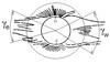 |
Fig. 1 Scheme showing how the angles defining parameter γ = 180 − (γW + γE) are found for the eclipse of 1923. The outer thin circle has a radius of 2 R⊙. |
The parameter γ is close to the index of the extent of the polar regions (Nikolskiy 1955; Loucif & Koutchmy 1989; Golub 2009). But in comparison with the polar index (Loucif & Koutchmy 1989), it is not calculated close to the limb, but at a height R⊙ above the solar limb. This allows taking the compression of coronal rays to the plane of which is the equator into account, possibly linked with non-radial spreading of the coronal streamers. This is especially significant for the minimum activity epoch (Tlatov 2010).
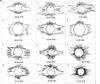 |
Fig. 2 Eclipses close to the minima of cycles 12–24. |
Figure 2 presents the shapes of eclipses for the epochs close to the solar activity minima of cycles 12–24. The calculated values of the parameter γ for these eclipses are listed in Table 1. The γ parameter varies within 40–100 degrees. Table 1 also gives the solar cycle phase Φ (see Eq. (1)). One can see that the highest magnitudes of the parameter γ occurred during the period 1934–1955. The remaining magnitudes fit the enveloping curve fairly well with a maximum during cycles 17–19 (see Fig. 3). No information on the solar corona structure during the eclipses at the minima of cycles 18 and 22 has been found in the literature. To fill the gaps, the eclipses during the phases of growth or decline of the solar cycle can be used. One can see in Table 1 that the eclipses of 1945 and 1984 are rather far from the minimum phase in solar activity. A modified parameter γ* = 180 − (γW + γE)·(1 − |Φ| ) can be introduced for these eclipses. This parameter reduces parameter γ to the minimum phase. The application of this procedure is effective for recognizing the shape of the corona close to the minimum activity with the phase Φ < 0.4. Figure 3 presents variations in parameter γ during the last 13 activity cycles.
Parameters γ for the eclipses of cycles 12–24.
3. Conclusions
The presence of long-term trends in the solar corona structure can be caused by changes in the configuration of the global magnetic field of the Sun. The role of active region formation during a solar activity minimum is not significant. It has long been known that large coronal streamers typically lie above the polarity-inversion lines of the large-scale magnetic field marked by filaments and prominences (Vsekhsvyatskiy et al. 1965). For this reason, investigations of the large-scale corona shape give valuable information on the structure of the large-scale fields during a long time interval. During the activity minimum, the properties of the global magnetic field of the Sun manifest themselves in the most pronounced way.
The magnetic field of the Sun is determined by large-scale structures. The northern and southern hemispheres of the Sun have magnetic fields of opposite polarity. The strength of the polar magnetic field is significantly higher than the fields in middle and low latitudes in the activity minimum period. Along with this, one can conclude from the analysis that assuming that the global solar field configuration is in the form of a dipole structure is probably incorrect. The corona configurations for the eclipses of 1889, 1901, and others correspond instead to the quadrupole form, or to an octopole form if different polarities at the poles are taken into account.
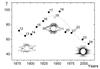 |
Fig. 3 Distribution of parameter γ. The structure of the corona for the epoch of minimum 13, 19, and 24 activity cycles are also shown. The dotted line is a 4th-order polynomial regression. |
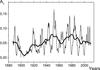 |
Fig. 4 Variations in the dipole moment derived from synoptic H-alpha charts of the Sun |


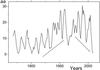 |
Fig. 5 Annual mean of the geomagnetic indices aa from 1868 (according to the National Geophysical Data Center, NGDC), smoothed by 2 years. The arrows mark the index growth in the first half of the 20th century and the index decrease during the last decades for the solar activity minimum epochs. |
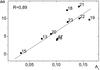 |
Fig. 6 Relation between the geomagnetic index aa and the magnitude of the dipole moment of the large-scale magnetic field A1 according to Figs. 4 and 5 during the solar activity minimum epoch. Numbers of activity cycles and linear regression are also shown. |
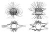 |
Fig. 7 Configuration of magnetic force lines for the corona of the dipole type (left) and quadrupole or octopole type if different polarities at the poles are considered (right). Regions of negative polarity are darkened. The structure of the corona for the epoch of minimum 13 and 19 activity cycles are also shown. |
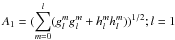
Thus, long-term variations in parameter γ should manifest changes in the dipole component during solar activity minima. This hypothesis can be checked using the data on configurations of the large-scale magnetic fields. Figure 4 shows changes in the dipole moment and the envelope drawn through solar activity minima. The data were obtained from the analysis of synoptic H-alpha charts of patterns of polarity inversion lines from Makarov & Sivaraman (1989), Vasileva (1998), and the Kislovodsk Astronomical Mountain Station (www.solarstation.ru). The greatest dipole moment corresponded to the minimum of cycle 19 in 1954. These data were obtained from H-alpha synoptic maps. The amplitude of the dipole contributions l = 1, which determine parameter A1 depend on the topology of the large-scale magnetic fields. The method of decomposition is given in Makarov & Tlatov (2000) and Tlatov (2009). On the whole, the envelope of the dipole moment shows similar trends in the changes in the corona shape parameter γ (see Figs. 3 and 4).
The growth in the strength of the radial component of the interplanetary magnetic field (Cliver & Ling 2002) determined from the geomagnetic activity index aa is another important problem that has been widely discussed recently. Figure 5 shows variations in the geomagnetic index aa. Data were taken from the National Geophysical Data Center2 (NGDC, http://www.ngdc.noaa.gov/). The first half of the 20th century was characterized by a growth in this index; i.e., the slowly varying component that was especially pronounced during the activity minimum epochs grew. During the past decades, a decrease in the aa index during the activity minimum epochs was observed. Probably, this is due to rearrangement of the global magnetic field of the Sun accompanied by changes in the solar corona structure during the minimum epochs. Variations in the geomagnetic index and the dipole moment of the large-scale magnetic field of the Sun during the activity minimum epoch are almost identical (see Fig. 6).
Thus, analysis of the corona shape has revealed a long-term modulation of the global magnetic field of the Sun. Possibly, a secular modulation exists of the global solar magnetic field that is most pronounced during the solar activity minimum epoch. During the secular cycle of the global magnetic field of the Sun, the relation between the dipole and octopole components of the magnetic field changes. The largest amplitude of the dipole component occurred during the interval 1944–1955. At the turn of the 19th to 20st and 20th to 21st centuries the solar corona shape and, possibly, the global magnetic field correspond to the configuration close to the octopole one (see Fig. 7).
The period of variation in the corona’s shape during the epoch of minimal activity is about 100–120 years (see Fig. 3), which is close to the Gleissberg cycle for the sunspots, but probably precedes it to some extent in phase (Hathaway 2010, Fig. 34). This conclusion does not contradict the calculations of the inclination angles of polar ray structures from the data on the large-scale fields with a maximum in 1940–1950 (Obridko & Shelting 1997). The maximum of the secular variation in the global magnetic field of the Sun occurred before cycle 19 and preceded the sunspot activity maximum. This allows us to put forward the hypothesis that secular variations in the solar activity are caused by secular modulation of the global magnetic field of the Sun. Another conclusion of this work is the supposition that the slowly changing component of the geomagnetic activity derived from the data on the aa index from changes in the dipole component of the large-scale field of the Sun (Fig. 6).
Eclipse photo of 01.08.2008 with permission of M. Druckmüller, http://www.zam.fme.vutbr.cz/~druck/Eclipse
Available through ftp (ftp://ftp.ngdc.noaa.gov/STP/GEOMAGNETIC_DATA/AASTAR/)
Acknowledgments
The work was work was supported by the Russian Foundation for Basic Research (RFBR) and the Program NS-3645.2010.2. The author thanks reviewer for improvements to style and language of this article.
References
- Cliver, E. W., & Ling, A. G. 2002, J. Geophys. Res., 107, SSH 11-1 [Google Scholar]
- Ganskiy, A. P. 1897, Proc. Royal. Akad. Sci. (in Russian), 6, 251 [Google Scholar]
- Golub, L., & Pasachoff, J. M. 2009, The Solar Corona, second edition (Cambridge University Press) [Google Scholar]
- Gulyaev, R. A. 1998, in Proc. Conf. A New Cycle of Solar Activity: Observations and Theoretical Aspects (in Russian), ed. A. V. Stepanov, Pulkovo, St. Petersburg, 61 [Google Scholar]
- Hathaway, D. H. 2010, Living Rev. Solar Phys., 7, http://solarscience.msfc.nasa.gov [Google Scholar]
- Loucif, M. L., & Koutchmy, S. 1989, A&AS, 77, 44 [Google Scholar]
- Makarov, V. I., & Sivaraman, K. R. 1989, Sol. Phys., 119, 35 [NASA ADS] [CrossRef] [Google Scholar]
- Makarov, V. I., & Tlatov, A. G. 2000, Astron. Rep., 44, 759 [NASA ADS] [CrossRef] [Google Scholar]
- Naegamvala, K. D. 1902, Report on the total solar eclipse of January 21–22, 1898, Bombay, 49 [Google Scholar]
- Nikolskiy, G. M. 1955, Astron. Cir., 160, 11 [Google Scholar]
- Obridko, V. N., & Shelting, B. D. 1997, in Proc. Conf. Modern Problems of Cyclicity (in Russian), ed. V. I. Makarov, Pulkovo, St. Petersburg, 193 [Google Scholar]
- Pasachoff, J. M., Rušin, V., Druckmüller, M., et al. 2008 , ApJ, 682, 638 [NASA ADS] [CrossRef] [Google Scholar]
- Tlatov, A. G. 2009, Sol. Phys., 260, 465 [Google Scholar]
- Tlatov, A. G. 2010, ApJ, 714, 805 [NASA ADS] [CrossRef] [Google Scholar]
- Vasileva, V. V. 1998, in Proc. Conf. A New Cycle of Solar Activity: Observations and Theoretical Aspects (in Russian), ed. A. V. Stepanov, Pulkovo, St. Petersburg, 213 [Google Scholar]
- Vsekhsvyatskiy, S. K., Nikolskiy, G. M., Ivanchuk, V. I., et al. 1965, Solar Corona and Corpuscular Radiation in the Interplanetary Space, Kiev, Naukova Dumka, 293 [Google Scholar]
- Waldmeier, M. 1976, Astron. Mitt. Eidgen. Sternw. Zurich, 351, 13 [NASA ADS] [Google Scholar]
All Tables
All Figures
|
Fig. 1 Scheme showing how the angles defining parameter γ = 180 − (γW + γE) are found for the eclipse of 1923. The outer thin circle has a radius of 2 R⊙. |
| In the text | |
|
Fig. 2 Eclipses close to the minima of cycles 12–24. |
| In the text | |
|
Fig. 3 Distribution of parameter γ. The structure of the corona for the epoch of minimum 13, 19, and 24 activity cycles are also shown. The dotted line is a 4th-order polynomial regression. |
| In the text | |
|
Fig. 4 Variations in the dipole moment derived from synoptic H-alpha charts of the Sun |
| In the text | |
|
Fig. 5 Annual mean of the geomagnetic indices aa from 1868 (according to the National Geophysical Data Center, NGDC), smoothed by 2 years. The arrows mark the index growth in the first half of the 20th century and the index decrease during the last decades for the solar activity minimum epochs. |
| In the text | |
|
Fig. 6 Relation between the geomagnetic index aa and the magnitude of the dipole moment of the large-scale magnetic field A1 according to Figs. 4 and 5 during the solar activity minimum epoch. Numbers of activity cycles and linear regression are also shown. |
| In the text | |
|
Fig. 7 Configuration of magnetic force lines for the corona of the dipole type (left) and quadrupole or octopole type if different polarities at the poles are considered (right). Regions of negative polarity are darkened. The structure of the corona for the epoch of minimum 13 and 19 activity cycles are also shown. |
| In the text | |
Current usage metrics show cumulative count of Article Views (full-text article views including HTML views, PDF and ePub downloads, according to the available data) and Abstracts Views on Vision4Press platform.
Data correspond to usage on the plateform after 2015. The current usage metrics is available 48-96 hours after online publication and is updated daily on week days.
Initial download of the metrics may take a while.